This capstone exercise ties together concepts from all six basics chapters. You will build a complete signal processing pipeline: acquire a noisy signal, analyse it, design a filter, apply it, and verify the result.
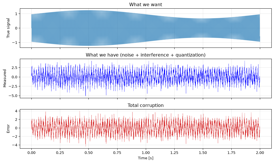
The scenario is realistic: a sensor measures a 200 Hz vibration signal, but the measurement is corrupted by broadband noise, a 50 Hz power-line interference tone, and quantization from a 12-bit ADC. Your job is to recover the signal.
The problem
import numpy as npimport matplotlib.pyplot as pltrng = np.random.default_rng(42)# System parameters (Chapter 1)fs =2000# sampling rate [Hz]duration =2# secondst = np.arange(duration * fs) / fs# The true signal: 200 Hz vibration with slow amplitude modulationsignal = (1+0.3* np.sin(2*np.pi*0.5*t)) * np.sin(2*np.pi*200*t)# Corruption 1: broadband sensor noise (Chapter 3)noise =0.8* rng.standard_normal(len(t))# Corruption 2: 50 Hz power-line interference (Chapter 3)interference =1.5* np.sin(2*np.pi*50*t +0.3)# Corruption 3: quantization (Chapter 1 + 3)def quantize(x, bits): scale =2** (bits -1)return np.clip(np.round(x * scale) / scale, -1.0, 1.0)raw = signal + noise + interference# Normalise to ADC range before quantizingraw_max = np.max(np.abs(raw))raw_norm = raw / raw_maxmeasured = quantize(raw_norm, 12) * raw_maxfig, axes = plt.subplots(3, 1, figsize=(10, 6), sharex=True)axes[0].plot(t, signal, 'C0-', linewidth=0.5)axes[0].set_ylabel('True signal')axes[0].set_title('What we want')axes[1].plot(t, measured, 'b-', linewidth=0.3)axes[1].set_ylabel('Measured')axes[1].set_title('What we have (noise + interference + quantization)')axes[2].plot(t, measured - signal, 'C3-', linewidth=0.3)axes[2].set_ylabel('Error')axes[2].set_title('Total corruption')axes[2].set_xlabel('Time [s]')for ax in axes: ax.grid(True, alpha=0.3)fig.tight_layout()plt.show()
Tasks
Work through these steps in order. Each one draws on a specific chapter.
Step 1: Characterise the corruption (Chapters 1, 3, 5)
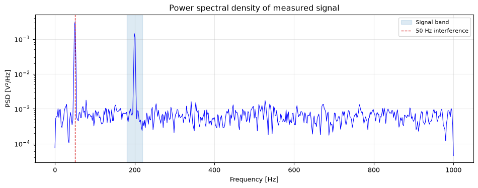
Compute the power spectrum of the measured signal using Welch’s method. Identify the signal component, the interference, and the noise floor.
Estimate the input SNR by comparing the signal power (in the 180–220 Hz band) with the total noise + interference power.
Is the noise white or colored? How can you tell from the PSD?
Estimated input SNR: -0.5 dB
The noise floor appears flat → white noise
Step 2: Remove the interference (Chapters 4, 6)
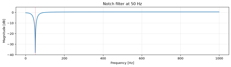
Design a notch filter at 50 Hz to remove the power-line interference. Place zeros on the unit circle at \(\theta = 2\pi \times 50/f_s\) and poles at the same angle with radius \(R = 0.95\).
Apply the notch filter. Verify the 50 Hz peak is gone from the PSD.
Step 3: Design and apply a bandpass filter (Chapter 6)
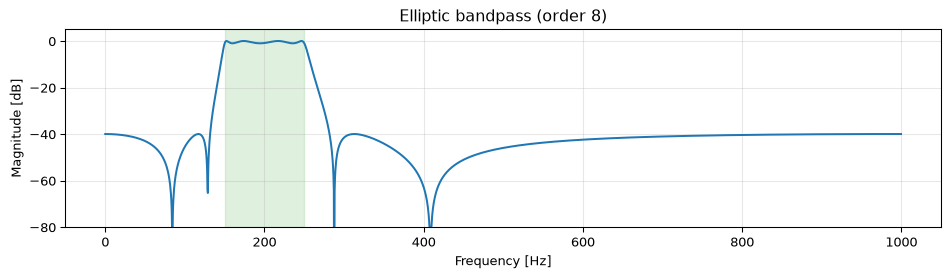
Design a bandpass filter to isolate the 200 Hz signal. Choose passband 150–250 Hz and stopband edges 100–300 Hz for safety margin around the modulated signal.
Use an elliptic IIR filter in SOS form. Find the minimum order.
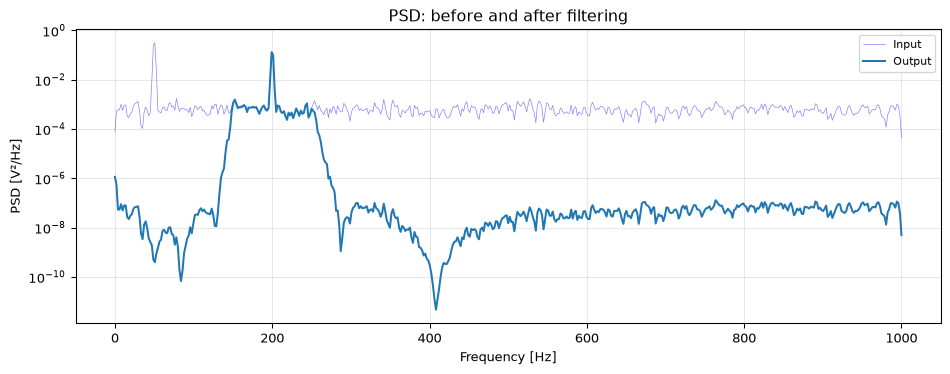
Input SNR (true):  -5.5 dB
Output SNR:        8.4 dB
Improvement:       13.9 dB
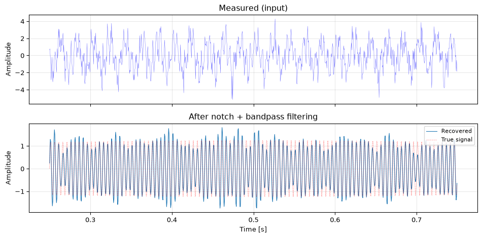
The filtering chain successfully recovers the amplitude-modulated 200 Hz tone. The startup transient is visible in the first ~250 ms (the IIR filter’s group delay). The recovered amplitude closely tracks the original modulation envelope.
Reflection questions
These don’t have single correct answers. They test your understanding of the trade-offs involved.
Why two filters instead of one? Could you use a single bandpass filter without the notch? What would you lose?
FIR alternative. If you replaced the IIR bandpass with an FIR filter, how many taps would you need for similar performance? What would be the advantage?
Averaging instead of filtering. The signal is periodic at 200 Hz. Could you use synchronous averaging (Ch3) instead of filtering? What information would you lose?
Quantization limit. The ADC is 12-bit. After all your filtering, can the output SNR ever exceed the quantization SNR of ~74 dB (for a full-scale sinusoid; other input statistics give different values)? Why or why not?
Real-time constraint. If this pipeline must run in real time on an embedded processor at \(f_s = 2000\) Hz, how many multiply-accumulate operations per sample does it require?
Source Code
---title: "Capstone: End-to-End Signal Processing"subtitle: "A mini-project tying together all six chapters"---This capstone exercise ties together concepts from all six basics chapters. You will build a complete signal processing pipeline: acquire a noisy signal, analyse it, design a filter, apply it, and verify the result.The scenario is realistic: a sensor measures a 200 Hz vibration signal, but the measurement is corrupted by broadband noise, a 50 Hz power-line interference tone, and quantization from a 12-bit ADC. Your job is to recover the signal.## The problem```{python}import numpy as npimport matplotlib.pyplot as pltrng = np.random.default_rng(42)# System parameters (Chapter 1)fs =2000# sampling rate [Hz]duration =2# secondst = np.arange(duration * fs) / fs# The true signal: 200 Hz vibration with slow amplitude modulationsignal = (1+0.3* np.sin(2*np.pi*0.5*t)) * np.sin(2*np.pi*200*t)# Corruption 1: broadband sensor noise (Chapter 3)noise =0.8* rng.standard_normal(len(t))# Corruption 2: 50 Hz power-line interference (Chapter 3)interference =1.5* np.sin(2*np.pi*50*t +0.3)# Corruption 3: quantization (Chapter 1 + 3)def quantize(x, bits): scale =2** (bits -1)return np.clip(np.round(x * scale) / scale, -1.0, 1.0)raw = signal + noise + interference# Normalise to ADC range before quantizingraw_max = np.max(np.abs(raw))raw_norm = raw / raw_maxmeasured = quantize(raw_norm, 12) * raw_maxfig, axes = plt.subplots(3, 1, figsize=(10, 6), sharex=True)axes[0].plot(t, signal, 'C0-', linewidth=0.5)axes[0].set_ylabel('True signal')axes[0].set_title('What we want')axes[1].plot(t, measured, 'b-', linewidth=0.3)axes[1].set_ylabel('Measured')axes[1].set_title('What we have (noise + interference + quantization)')axes[2].plot(t, measured - signal, 'C3-', linewidth=0.3)axes[2].set_ylabel('Error')axes[2].set_title('Total corruption')axes[2].set_xlabel('Time [s]')for ax in axes: ax.grid(True, alpha=0.3)fig.tight_layout()plt.show()```## TasksWork through these steps in order. Each one draws on a specific chapter.### Step 1: Characterise the corruption (Chapters 1, 3, 5)a) Compute the **power spectrum** of the measured signal using Welch's method. Identify the signal component, the interference, and the noise floor.b) Estimate the **input SNR** by comparing the signal power (in the 180–220 Hz band) with the total noise + interference power.c) Is the noise white or colored? How can you tell from the PSD?::: {.callout-note collapse="true" title="Solution"}```{python}from scipy.signal import welchf, psd = welch(measured, fs, nperseg=1024)fig, ax = plt.subplots(figsize=(10, 4))ax.semilogy(f, psd, 'b-', linewidth=0.8)ax.axvspan(180, 220, alpha=0.15, color='C0', label='Signal band')ax.axvline(50, color='C3', linewidth=1, linestyle='--', label='50 Hz interference')ax.set_xlabel('Frequency [Hz]')ax.set_ylabel('PSD [V²/Hz]')ax.set_title('Power spectral density of measured signal')ax.legend(fontsize=8)ax.grid(True, alpha=0.3)fig.tight_layout()plt.show()# SNR estimatesignal_mask = (f >=180) & (f <=220)noise_mask = (f >0) &~signal_mask &~((f >=45) & (f <=55)) # exclude interference peakp_sig = np.sum(psd[signal_mask]) * (f[1] - f[0])p_noise = np.sum(psd[noise_mask]) * (f[1] - f[0])snr_in =10* np.log10(p_sig / p_noise)print(f"Estimated input SNR: {snr_in:.1f} dB")print("The noise floor appears flat → white noise")```:::### Step 2: Remove the interference (Chapters 4, 6)a) Design a **notch filter** at 50 Hz to remove the power-line interference. Place zeros on the unit circle at $\theta = 2\pi \times 50/f_s$ and poles at the same angle with radius $R = 0.95$.b) Apply the notch filter. Verify the 50 Hz peak is gone from the PSD.::: {.callout-note collapse="true" title="Solution"}```{python}from scipy.signal import freqz, lfilter# Notch filter (Chapter 4: pole-zero placement)theta =2* np.pi *50/ fsR =0.95b_notch = [1, -2*np.cos(theta), 1]a_notch = [1, -2*R*np.cos(theta), R**2]# Verify frequency responsew, H_notch = freqz(b_notch, a_notch, worN=2048, fs=fs)fig, ax = plt.subplots(figsize=(10, 3))ax.plot(w, 20*np.log10(np.maximum(np.abs(H_notch), 1e-10)), 'C0-', linewidth=1.5)ax.axvline(50, color='C3', linewidth=0.5, linestyle='--')ax.set_xlabel('Frequency [Hz]')ax.set_ylabel('Magnitude [dB]')ax.set_ylim(-40, 5)ax.set_title('Notch filter at 50 Hz')ax.grid(True, alpha=0.3)fig.tight_layout()plt.show()# Apply (2nd-order filter is numerically stable in direct form)deinterfered = lfilter(b_notch, a_notch, measured)```:::### Step 3: Design and apply a bandpass filter (Chapter 6)a) Design a **bandpass filter** to isolate the 200 Hz signal. Choose passband 150–250 Hz and stopband edges 100–300 Hz for safety margin around the modulated signal.b) Use an elliptic IIR filter in SOS form. Find the minimum order.c) Apply the filter using `sosfilt`.::: {.callout-note collapse="true" title="Solution"}```{python}from scipy.signal import ellipord, ellip, sosfilt, sosfreqz# Design (Chapter 6)N, Wn = ellipord([150, 250], [100, 300], 1, 40, fs=fs)sos = ellip(N, 1, 40, Wn, btype='band', fs=fs, output='sos')print(f"Elliptic bandpass: order {2*N} ({N} prototype, doubled for bandpass)")# Verifyw, H_bp = sosfreqz(sos, worN=2048, fs=fs)fig, ax = plt.subplots(figsize=(10, 3))ax.plot(w, 20*np.log10(np.maximum(np.abs(H_bp), 1e-10)), 'C0-', linewidth=1.5)ax.axvspan(150, 250, alpha=0.15, color='C2')ax.set_xlabel('Frequency [Hz]')ax.set_ylabel('Magnitude [dB]')ax.set_ylim(-80, 5)ax.set_title(f'Elliptic bandpass (order {2*N})')ax.grid(True, alpha=0.3)fig.tight_layout()plt.show()# Applyrecovered = sosfilt(sos, deinterfered)```:::### Step 4: Evaluate the result (Chapters 3, 5)a) Compare the **output PSD** with the input PSD. Has the noise floor dropped? Is the 50 Hz peak gone?b) Compute the **output SNR**. How much did filtering improve it?c) Plot the recovered signal overlaid with the original. Identify any remaining artifacts (startup transient, amplitude distortion from passband ripple).::: {.callout-note collapse="true" title="Solution"}```{python}# a) PSD comparisonf_out, psd_out = welch(recovered, fs, nperseg=1024)fig, ax = plt.subplots(figsize=(10, 4))ax.semilogy(f, psd, 'b-', linewidth=0.5, alpha=0.5, label='Input')ax.semilogy(f_out, psd_out, 'C0-', linewidth=1.5, label='Output')ax.set_xlabel('Frequency [Hz]')ax.set_ylabel('PSD [V²/Hz]')ax.set_title('PSD: before and after filtering')ax.legend(fontsize=8)ax.grid(True, alpha=0.3)fig.tight_layout()plt.show()# b) Output SNR (filter the true signal and noise separately)sig_filtered = sosfilt(sos, lfilter(b_notch, a_notch, signal))noise_filtered = sosfilt(sos, lfilter(b_notch, a_notch, noise + interference))skip =500# skip transientp_sig_out = np.mean(sig_filtered[skip:]**2)p_noise_out = np.mean(noise_filtered[skip:]**2)snr_out =10* np.log10(p_sig_out / p_noise_out)p_sig_in = np.mean(signal[skip:]**2)p_noise_in = np.mean((noise[skip:] + interference[skip:])**2)snr_in_true =10* np.log10(p_sig_in / p_noise_in)print(f"Input SNR (true): {snr_in_true:.1f} dB")print(f"Output SNR: {snr_out:.1f} dB")print(f"Improvement: {snr_out - snr_in_true:.1f} dB")# c) Time-domain comparisonfig, axes = plt.subplots(2, 1, figsize=(10, 5), sharex=True)t_plot =slice(500, 1500) # skip transient, show 0.5 secondsaxes[0].plot(t[t_plot], measured[t_plot], 'b-', linewidth=0.3, alpha=0.7)axes[0].set_ylabel('Amplitude')axes[0].set_title('Measured (input)')axes[1].plot(t[t_plot], recovered[t_plot], 'C0-', linewidth=0.8, label='Recovered')axes[1].plot(t[t_plot], signal[t_plot], 'r--', linewidth=0.5, alpha=0.5, label='True signal')axes[1].set_ylabel('Amplitude')axes[1].set_xlabel('Time [s]')axes[1].set_title('After notch + bandpass filtering')axes[1].legend(fontsize=8)for ax in axes: ax.grid(True, alpha=0.3)fig.tight_layout()plt.show()```The filtering chain successfully recovers the amplitude-modulated 200 Hz tone. The startup transient is visible in the first ~250 ms (the IIR filter's group delay). The recovered amplitude closely tracks the original modulation envelope.:::## Reflection questionsThese don't have single correct answers. They test your understanding of the trade-offs involved.1. **Why two filters instead of one?** Could you use a single bandpass filter without the notch? What would you lose?2. **FIR alternative.** If you replaced the IIR bandpass with an FIR filter, how many taps would you need for similar performance? What would be the advantage?3. **Averaging instead of filtering.** The signal is periodic at 200 Hz. Could you use synchronous averaging (Ch3) instead of filtering? What information would you lose?4. **Quantization limit.** The ADC is 12-bit. After all your filtering, can the output SNR ever exceed the quantization SNR of ~74 dB (for a full-scale sinusoid; other input statistics give different values)? Why or why not?5. **Real-time constraint.** If this pipeline must run in real time on an embedded processor at $f_s = 2000$ Hz, how many multiply-accumulate operations per sample does it require?