Chapters 2 and 4 taught you what filters are: difference equations, transfer functions, poles and zeros. Chapter 5 showed you how to analyse filters in the frequency domain. This chapter is about designing them: given a set of requirements, how do you find coefficients that meet those requirements?
We’ll cover two families:
FIR filters, designed by windowing or optimization, always stable, can have perfectly linear phase.
IIR filters, designed by transforming classical analog prototypes, much more efficient (fewer coefficients for the same sharpness), but phase is nonlinear and stability must be checked.
Both families are handled by scipy.signal, so you rarely need to implement the algorithms yourself. The goal here is to understand what you’re asking the computer to do, and why certain choices lead to better filters.
Filter specifications
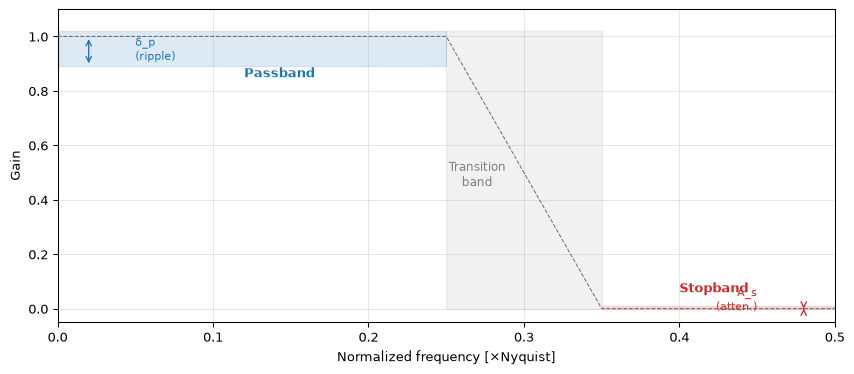
Before you can design a filter, you need to say what you want. A lowpass filter specification typically includes:
Passband edge\(f_p\): frequencies below this should pass through.
Stopband edge\(f_s\): frequencies above this should be blocked.
Passband ripple\(\delta_p\) (in dB): how much variation is acceptable in the passband.
Stopband attenuation\(A_s\) (in dB): how much the filter must suppress signals in the stopband.
The gap between \(f_p\) and \(f_s\) is the transition band, the region where the filter transitions from passing to blocking. A narrower transition band requires a higher-order filter (more coefficients, more computation).
Figure 1: Anatomy of a lowpass filter specification. The passband ripple and stopband attenuation define how tightly the filter must meet the ideal response.
The design triangle
There is a fundamental trade-off between three quantities:
Transition width (how sharp the cutoff is)
Ripple (how flat the passband and stopband are)
Filter order (how many coefficients you need)
You can pick any two, and the third is determined by the design algorithm. Want a sharper cutoff and less ripple? You’ll need a higher order filter. Want to keep the order low? Either widen the transition band or accept more ripple.
Other filter types
Everything we say about lowpass filters extends naturally:
Type
What it passes
How to derive
Lowpass
\(0\) to \(f_p\)
Base design
Highpass
\(f_p\) to \(f_\text{nyq}\)
Spectral inversion of lowpass
Bandpass
\(f_1\) to \(f_2\)
Two cutoffs
Bandstop (notch)
Everything except\(f_1\) to \(f_2\)
Complement of bandpass
scipy’s design functions (firwin, butter, cheby1, etc.) accept a btype parameter for all four types.
FIR filter design
FIR filters are attractive because they are:
Always stable: no feedback means no poles outside the unit circle.
Easily made linear phase: a symmetric impulse response gives constant group delay.
The price is filter length: FIR filters typically need many more coefficients than an IIR filter for the same transition width.
The window method
The idea is elegant. An ideal lowpass filter has a sinc impulse response, but it’s infinitely long, so we can’t use it directly. The window method simply truncates the sinc and applies a window function to reduce the resulting spectral leakage.
The ideal discrete-time lowpass impulse response with cutoff \(f_c\) is:
\[h_\text{ideal}[n] = \frac{\sin(2\pi f_c n / f_s)}{\pi n}\]
Truncating to \(N\) samples and centring gives a causal FIR filter. Multiplying by a window (Hamming, Blackman, Kaiser, …) trades main-lobe width for side-lobe suppression, exactly the same trade-off we saw in Chapter 5 for spectral analysis.
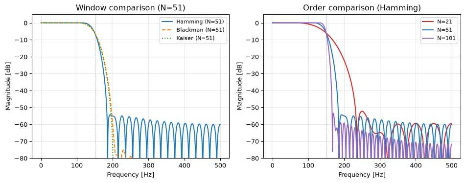
scipy.signal.firwin does all of this in one call:
fs =1000f_cutoff =150# Hzfig, axes = plt.subplots(1, 2, figsize=(10, 4))for window, color, ls in [('hamming', 'C0', '-'), ('blackman', 'C1', '--'), ('kaiser', 'C2', ':')]:if window =='kaiser': h = firwin(51, f_cutoff, fs=fs, window=('kaiser', 8.0))else: h = firwin(51, f_cutoff, fs=fs, window=window) w, H = freqz(h, [1], worN=2048, fs=fs) axes[0].plot(w, 20*np.log10(np.maximum(np.abs(H), 1e-10)), color=color, linestyle=ls, linewidth=1.5, label=f'{window.capitalize()} (N=51)')axes[0].set_xlabel('Frequency [Hz]')axes[0].set_ylabel('Magnitude [dB]')axes[0].set_ylim(-80, 5)axes[0].axvline(f_cutoff, color='gray', linewidth=0.5, linestyle='--')axes[0].legend(fontsize=8)axes[0].grid(True, alpha=0.3)axes[0].set_title('Window comparison (N=51)')# Effect of filter orderfor N, color in [(21, 'C3'), (51, 'C0'), (101, 'C4')]: h = firwin(N, f_cutoff, fs=fs, window='hamming') w, H = freqz(h, [1], worN=2048, fs=fs) axes[1].plot(w, 20*np.log10(np.maximum(np.abs(H), 1e-10)), color=color, linewidth=1.5, label=f'N={N}')axes[1].set_xlabel('Frequency [Hz]')axes[1].set_ylabel('Magnitude [dB]')axes[1].set_ylim(-80, 5)axes[1].axvline(f_cutoff, color='gray', linewidth=0.5, linestyle='--')axes[1].legend(fontsize=8)axes[1].grid(True, alpha=0.3)axes[1].set_title('Order comparison (Hamming)')fig.tight_layout()plt.show()
Figure 2: FIR lowpass filters designed with firwin using different window functions. Sharper transition requires either more taps or accepts more ripple.
The Parks–McClellan method (equiripple)
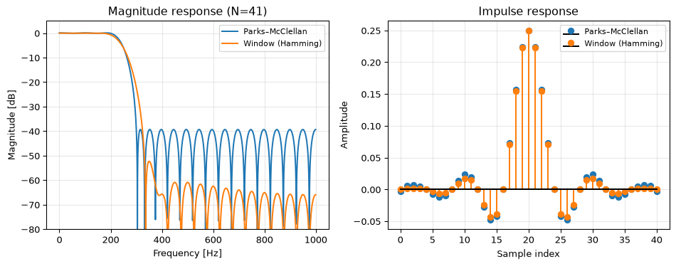
The window method doesn’t let you control passband and stopband ripple independently. The Parks–McClellan algorithm (also called the Remez exchange algorithm) designs FIR filters that minimise the maximum error, producing equiripple behaviour in both bands.
You specify:
Band edges (where passband ends and stopband begins)
Desired gain in each band
Relative weighting (how much you care about each band)
The algorithm then finds the optimal coefficients for a given filter order (Proakis and Manolakis 2007).
Figure 3: Equiripple FIR filter designed with remez. The ripple is distributed evenly across passband and stopband, optimal for meeting a given specification with minimum order.
Linear phase and group delay
A key advantage of FIR filters: if the impulse response is symmetric (\(h[n] = h[N-1-n]\)), the filter has exactly linear phase. This means all frequencies experience the same delay: no phase distortion. Both firwin and remez produce symmetric coefficients by default.
The group delay formalizes this concept. It is defined as the negative derivative of the phase response:
\[\tau(\omega) = -\frac{d\phi(\omega)}{d\omega}\]
where \(\phi(\omega) = \angle H(e^{j\omega T})\) is the phase response. Group delay tells you how much each frequency component is delayed by the filter, measured in samples. For a linear-phase FIR filter, the phase is a straight line, so the derivative is constant: \(\tau = (N-1)/2\) samples at all frequencies.
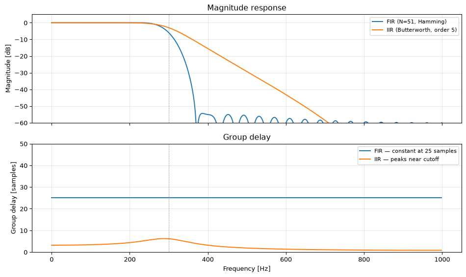
IIR filters have non-constant group delay: different frequencies are delayed by different amounts. This causes waveform distortion even when the magnitude response is flat. The effect is especially pronounced near the cutoff frequency, where the group delay can peak sharply.
from scipy.signal import group_delayfs =2000fc =300# FIR: 51-tap Hamming lowpassh_fir = firwin(51, fc, fs=fs)w_fir, gd_fir = group_delay(([*h_fir], [1]), fs=fs)# IIR: 5th-order Butterworth lowpassb_iir, a_iir = butter(5, fc, fs=fs)w_iir, gd_iir = group_delay((b_iir, a_iir), fs=fs)fig, axes = plt.subplots(2, 1, figsize=(10, 6), sharex=True)# Magnitude responsefor b, a, label, color in [([*h_fir], [1], 'FIR (N=51, Hamming)', 'C0'), (b_iir, a_iir, 'IIR (Butterworth, order 5)', 'C1')]: w, H = freqz(b, a, worN=2048, fs=fs) axes[0].plot(w, 20*np.log10(np.maximum(np.abs(H), 1e-10)), color=color, linewidth=1.5, label=label)axes[0].set_ylabel('Magnitude [dB]')axes[0].set_ylim(-60, 5)axes[0].axvline(fc, color='gray', linewidth=0.5, linestyle='--')axes[0].legend(fontsize=8)axes[0].grid(True, alpha=0.3)axes[0].set_title('Magnitude response')# Group delayaxes[1].plot(w_fir, gd_fir, 'C0-', linewidth=1.5, label='FIR — constant at 25 samples')axes[1].plot(w_iir, gd_iir, 'C1-', linewidth=1.5, label='IIR — peaks near cutoff')axes[1].set_ylabel('Group delay [samples]')axes[1].set_xlabel('Frequency [Hz]')axes[1].axvline(fc, color='gray', linewidth=0.5, linestyle='--')axes[1].set_ylim(0, max(gd_iir.max() *1.2, 50))axes[1].legend(fontsize=8)axes[1].grid(True, alpha=0.3)axes[1].set_title('Group delay')fig.tight_layout()plt.show()
Figure 4: Group delay comparison: a linear-phase FIR filter (constant delay) vs a Butterworth IIR filter (frequency-dependent delay, peaking near cutoff).
The FIR filter has perfectly flat group delay: all frequencies arrive at the same time. The IIR filter’s group delay peaks sharply near the cutoff, meaning frequencies close to the transition band are delayed more than others. This frequency-dependent delay distorts transient signals (like speech or ECG waveforms). When phase distortion matters, either use a linear-phase FIR or apply sosfiltfilt for zero-phase IIR filtering (offline only).
Exercise: FIR order estimation
You need a lowpass filter with \(f_p = 1000\) Hz, \(f_{\text{stop}} = 1200\) Hz, and 40 dB stopband attenuation at \(f_s = 8000\) Hz sampling rate.
What is the normalised transition width \(\Delta f / f_s\)?
Using the rule of thumb \(N \approx A_s / (22 \cdot \Delta f / f_s)\), estimate the required filter order.
Design the filter with firwin using a Kaiser window (beta=5.65 for 40 dB) and verify the stopband attenuation.
h = firwin(73, 1100, fs=8000, window=('kaiser', 5.65))w, H = freqz(h, [1], worN=2048, fs=8000)H_dB =20* np.log10(np.maximum(np.abs(H), 1e-10))# Check attenuation at stopband edgeidx_stop = np.argmin(np.abs(w -1200))print(f"Attenuation at 1200 Hz: {-H_dB[idx_stop]:.1f} dB")print(f"Worst-case stopband: {-np.min(H_dB[w >=1200]):.1f} dB")
Attenuation at 1200 Hz: 18.6 dB
Worst-case stopband: 144.7 dB
IIR filter design
FIR filters need many taps for a sharp cutoff. A 100th-order FIR filter requires 101 multiply-accumulate operations per sample. An IIR filter can achieve a comparable response with order 5–10, using only about 15–25 operations, a significant advantage in real-time or embedded applications.
The standard approach to IIR filter design is:
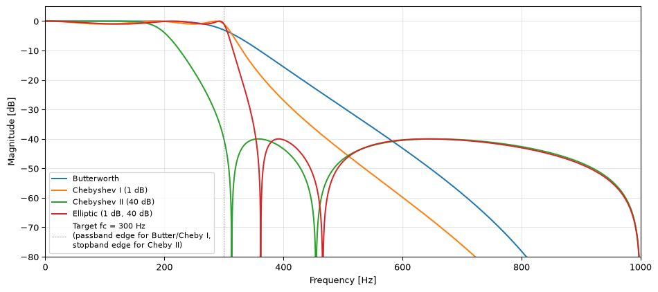
Start with a classical analog prototype filter (Butterworth, Chebyshev, or Elliptic).
Transform it to digital using the bilinear transform.
The result is a set of coefficients \((b, a)\) in z-domain form.
scipy’s butter, cheby1, cheby2, and ellip functions handle all three steps internally.
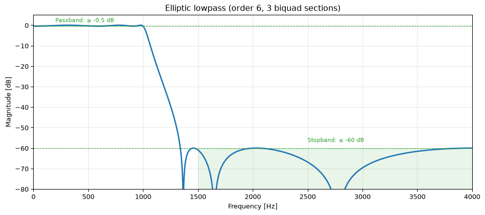
Figure 5: The four classical IIR filter families applied to the same specification. Elliptic achieves the sharpest transition at the cost of ripple in both bands.
Family
Passband
Stopband
Transition
Use when
Butterworth
Maximally flat
Maximally flat
Widest
Flatness matters most
Chebyshev I
Equiripple
Monotonic
Narrower
Some passband ripple is acceptable
Chebyshev II
Monotonic
Equiripple
Narrower
Flat passband needed, stopband ripple OK
Elliptic
Equiripple
Equiripple
Narrowest
Minimum order is the priority
The bilinear transform
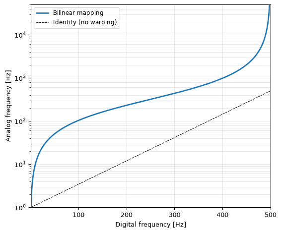
All these designs start from analog prototypes, continuous-time filters with transfer functions in the Laplace domain \(H_a(s)\). The bilinear transform(Mitra 2006) converts them to discrete-time by substituting:
\[s \leftarrow \frac{2}{T}\,\frac{z-1}{z+1}\]
This mapping has two key properties:
Stability is preserved: the left half of the \(s\)-plane maps to the interior of the unit circle.
Frequency is warped: the linear frequency axis of the analog filter is compressed onto the finite interval \([0, f_\text{nyq}]\) via the relation:
At low frequencies this warping is negligible, but near Nyquist the compression is severe. scipy’s design functions automatically pre-warp the critical frequencies to compensate; you specify frequencies in Hz and the functions handle the rest.
Figure 6: Frequency warping of the bilinear transform. The mapping is nearly linear at low frequencies but compresses sharply near Nyquist.
Exercise: Butterworth vs Chebyshev order
You need a lowpass filter with passband edge 500 Hz, stopband edge 750 Hz, at most 1 dB passband ripple, and at least 40 dB stopband attenuation. Sampling rate is 4000 Hz.
Use scipy.signal.buttord to find the minimum Butterworth order.
Chebyshev I achieves the same specification with a lower order because it allows ripple in the passband. Butterworth’s maximally-flat constraint forces a wider transition band for the same order.
Second-order sections (biquads)
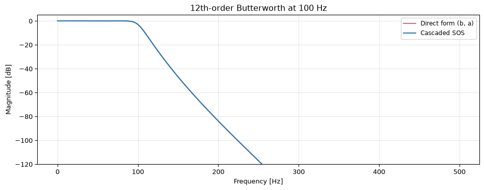
High-order IIR filters implemented directly as a single \((b, a)\) polynomial pair are numerically fragile. Small rounding errors in the coefficients can shift poles outside the unit circle, causing instability. This is especially dangerous with orders above 6–8.
The solution: cascade second-order sections (SOS), also called biquads(Mitra 2006). Each section is a second-order filter:
The overall filter is the product \(H(z) = \prod_k H_k(z)\). Each biquad has at most 2 poles, so rounding errors only affect a small, well-conditioned sub-problem.
fs =1000fc =100order =12# Direct form (b, a)b, a = butter(order, fc, fs=fs)w_ba, H_ba = freqz(b, a, worN=2048, fs=fs)# SOS formsos = butter(order, fc, fs=fs, output='sos')w_sos, H_sos = sosfreqz(sos, worN=2048, fs=fs)fig, ax = plt.subplots(figsize=(10, 4))ax.plot(w_ba, 20*np.log10(np.maximum(np.abs(H_ba), 1e-10)),'C3-', linewidth=1.5, alpha=0.7, label='Direct form (b, a)')ax.plot(w_sos, 20*np.log10(np.maximum(np.abs(H_sos), 1e-10)),'C0-', linewidth=1.5, label='Cascaded SOS')ax.set_xlabel('Frequency [Hz]')ax.set_ylabel('Magnitude [dB]')ax.set_ylim(-120, 5)ax.legend(fontsize=9)ax.grid(True, alpha=0.3)ax.set_title(f'12th-order Butterworth at {fc} Hz')fig.tight_layout()plt.show()
Figure 7: Numerical stability: a 12th-order Butterworth filter implemented as (b,a) coefficients vs cascaded second-order sections (SOS). The direct form shows severe numerical artifacts.
Important
Always use SOS form for IIR filters of order 4 and above. Pass output='sos' to the design functions, and use sosfilt instead of lfilter for filtering.
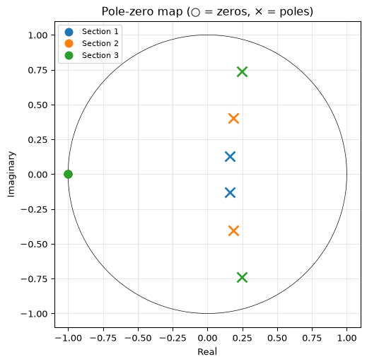
Figure 8: Pole-zero map of a 6th-order Butterworth lowpass. Each biquad section contributes one conjugate pole pair (and corresponding zeros), keeping poles well inside the unit circle.
See these filters running on real microcontrollers: the biquad embedded page shows IIR cascades and FIR circular buffers on STM32F4 and ESP32-S3, with cycle counts and memory comparisons. The multirate embedded page demonstrates FIR decimation and multiply-free CIC filters.
Rules of thumb:
Need linear phase or guaranteed stability? → FIR
Tight real-time budget or embedded system? → IIR
Offline processing where phase doesn’t matter? → IIR (simpler, then sosfiltfilt for zero-phase)
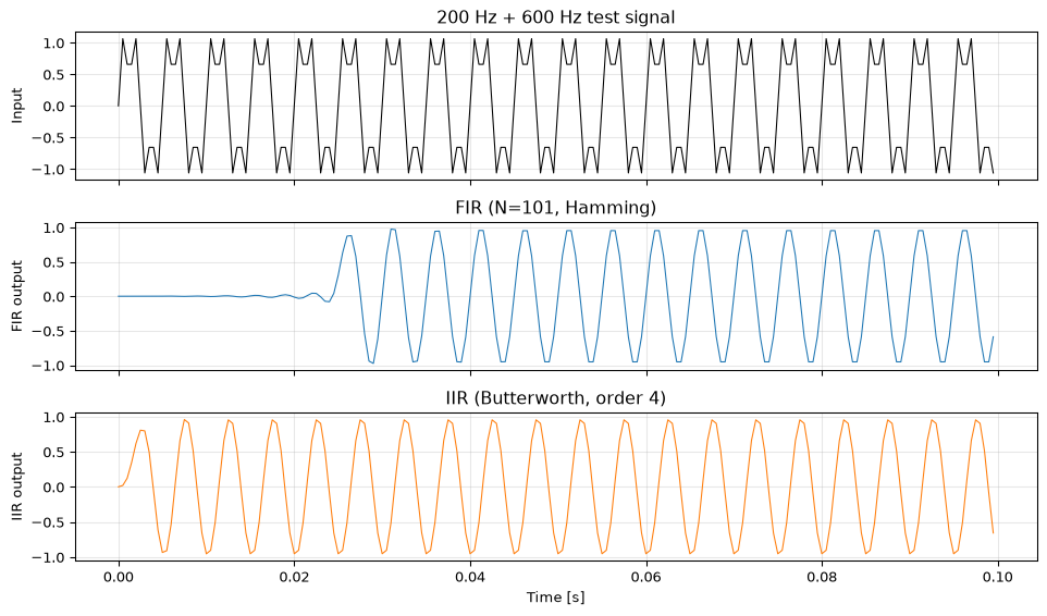
Both filters remove the 600 Hz component. The FIR output has a visible startup delay of \((101-1)/2 = 50\) samples, while the IIR filter responds almost immediately but with a brief transient.
Practical design with Python
Here’s a complete workflow for designing a filter to meet a specification.
Butterworth (flat), Chebyshev (ripple in one band), Elliptic (ripple in both)
Group delay
\(\tau(\omega) = -d\phi/d\omega\), constant for linear-phase FIR, variable for IIR
Bilinear transform
\(s\)-plane → \(z\)-plane with frequency warping
SOS / biquads
Cascade 2nd-order sections for numerical stability
sosfilt
Always use SOS form for IIR filtering
The next step is to apply these tools to real problems: removing power-line interference, designing audio equalizers, building anti-aliasing filters for data acquisition. The Topics section explores several of these applications.
Further reading
Proakis & Manolakis, Digital Signal Processing (2007), Ch. 8: IIR filter design, Ch. 10: FIR filter design
Mitra, Digital Signal Processing (2006), Ch. 7.3–7.5: Bilinear transform, SOS form, Parks-McClellan
Going deeper
The biquad filters topic covers efficient second-order section implementations for embedded systems. Adaptive filtering extends filter design to systems that adjust their coefficients in real time.
References
Mitra, Sanjit K. 2006. Digital Signal Processing: A Computer-Based Approach. 3rd ed. McGraw-Hill.
Proakis, John G., and Dimitris G. Manolakis. 2007. Digital Signal Processing: Principles, Algorithms, and Applications. 4th ed. Pearson.
Source Code
---title: "Filter Design"subtitle: "From specifications to working filters"---```{python}#| echo: falseimport numpy as npimport matplotlib.pyplot as pltfrom scipy.signal import (freqz, sosfreqz, firwin, remez, butter, cheby1, cheby2, ellip, lfilter, sosfilt, tf2zpk)```Chapters 2 and 4 taught you what filters *are*: difference equations, transfer functions, poles and zeros. Chapter 5 showed you how to *analyse* filters in the frequency domain. This chapter is about *designing* them: given a set of requirements, how do you find coefficients that meet those requirements?We'll cover two families:- **FIR filters**, designed by windowing or optimization, always stable, can have perfectly linear phase.- **IIR filters**, designed by transforming classical analog prototypes, much more efficient (fewer coefficients for the same sharpness), but phase is nonlinear and stability must be checked.Both families are handled by `scipy.signal`, so you rarely need to implement the algorithms yourself. The goal here is to understand *what* you're asking the computer to do, and *why* certain choices lead to better filters.---## Filter specificationsBefore you can design a filter, you need to say what you want. A lowpass filter specification typically includes:- **Passband edge** $f_p$: frequencies below this should pass through.- **Stopband edge** $f_s$: frequencies above this should be blocked.- **Passband ripple** $\delta_p$ (in dB): how much variation is acceptable in the passband.- **Stopband attenuation** $A_s$ (in dB): how much the filter must suppress signals in the stopband.The gap between $f_p$ and $f_s$ is the **transition band**, the region where the filter transitions from passing to blocking. A narrower transition band requires a higher-order filter (more coefficients, more computation).```{python}#| label: fig-filter-spec#| fig-cap: "Anatomy of a lowpass filter specification. The passband ripple and stopband attenuation define how tightly the filter must meet the ideal response."fig, ax = plt.subplots(figsize=(9, 4))# Ideal responsef_pass, f_stop =0.25, 0.35freqs = [0, f_pass, f_pass, f_stop, f_stop, 0.5]ideal = [1, 1, 1, 0, 0, 0]ax.plot(freqs, ideal, 'k--', linewidth=0.8, alpha=0.5, label='Ideal')# Specification bandsrp_lin =10**(-1/20) # 1 dB rippleax.fill_between([0, f_pass], 1+0.02, rp_lin, color='C0', alpha=0.15)ax.fill_between([f_stop, 0.5], 10**(-40/20), 0, color='C3', alpha=0.15)ax.fill_between([f_pass, f_stop], 0, 1.02, color='C7', alpha=0.1)# Annotationsax.annotate('Passband', xy=(0.12, 0.85), fontsize=10, color='C0', fontweight='bold')ax.annotate('Stopband', xy=(0.4, 0.06), fontsize=10, color='C3', fontweight='bold')ax.annotate('Transition\nband', xy=(0.27, 0.45), fontsize=9, color='gray', ha='center')ax.annotate('', xy=(0.02, rp_lin), xytext=(0.02, 1.0), arrowprops=dict(arrowstyle='<->', color='C0'))ax.text(0.05, 0.95, f'δ_p\n(ripple)', fontsize=8, color='C0', va='center')ax.annotate('', xy=(0.48, 0), xytext=(0.48, 10**(-40/20)), arrowprops=dict(arrowstyle='<->', color='C3'))ax.text(0.45, 0.03, 'A_s\n(atten.)', fontsize=8, color='C3', va='center', ha='right')ax.set_xlabel('Normalized frequency [×Nyquist]')ax.set_ylabel('Gain')ax.set_xlim(0, 0.5)ax.set_ylim(-0.05, 1.1)ax.grid(True, alpha=0.3)fig.tight_layout()plt.show()```### The design triangleThere is a fundamental trade-off between three quantities:1. **Transition width** (how sharp the cutoff is)2. **Ripple** (how flat the passband and stopband are)3. **Filter order** (how many coefficients you need)You can pick any two, and the third is determined by the design algorithm. Want a sharper cutoff *and* less ripple? You'll need a higher order filter. Want to keep the order low? Either widen the transition band or accept more ripple.### Other filter typesEverything we say about lowpass filters extends naturally:| Type | What it passes | How to derive ||------|---------------|---------------|| **Lowpass** | $0$ to $f_p$ | Base design || **Highpass** | $f_p$ to $f_\text{nyq}$ | Spectral inversion of lowpass || **Bandpass** | $f_1$ to $f_2$ | Two cutoffs || **Bandstop** (notch) | Everything *except* $f_1$ to $f_2$ | Complement of bandpass |scipy's design functions (`firwin`, `butter`, `cheby1`, etc.) accept a `btype` parameter for all four types.---## FIR filter designFIR filters are attractive because they are:- **Always stable**: no feedback means no poles outside the unit circle.- **Easily made linear phase**: a symmetric impulse response gives constant group delay.The price is filter length: FIR filters typically need many more coefficients than an IIR filter for the same transition width.### The window methodThe idea is elegant. An ideal lowpass filter has a sinc impulse response, but it's infinitely long, so we can't use it directly. The window method simply **truncates** the sinc and applies a **window function** to reduce the resulting spectral leakage.The ideal discrete-time lowpass impulse response with cutoff $f_c$ is:$$h_\text{ideal}[n] = \frac{\sin(2\pi f_c n / f_s)}{\pi n}$$Truncating to $N$ samples and centring gives a causal FIR filter. Multiplying by a window (Hamming, Blackman, Kaiser, ...) trades main-lobe width for side-lobe suppression, exactly the same trade-off we saw in [Chapter 5](05-frequency-domain.qmd) for spectral analysis.`scipy.signal.firwin` does all of this in one call:```{python}#| label: fig-fir-window#| fig-cap: "FIR lowpass filters designed with firwin using different window functions. Sharper transition requires either more taps or accepts more ripple."fs =1000f_cutoff =150# Hzfig, axes = plt.subplots(1, 2, figsize=(10, 4))for window, color, ls in [('hamming', 'C0', '-'), ('blackman', 'C1', '--'), ('kaiser', 'C2', ':')]:if window =='kaiser': h = firwin(51, f_cutoff, fs=fs, window=('kaiser', 8.0))else: h = firwin(51, f_cutoff, fs=fs, window=window) w, H = freqz(h, [1], worN=2048, fs=fs) axes[0].plot(w, 20*np.log10(np.maximum(np.abs(H), 1e-10)), color=color, linestyle=ls, linewidth=1.5, label=f'{window.capitalize()} (N=51)')axes[0].set_xlabel('Frequency [Hz]')axes[0].set_ylabel('Magnitude [dB]')axes[0].set_ylim(-80, 5)axes[0].axvline(f_cutoff, color='gray', linewidth=0.5, linestyle='--')axes[0].legend(fontsize=8)axes[0].grid(True, alpha=0.3)axes[0].set_title('Window comparison (N=51)')# Effect of filter orderfor N, color in [(21, 'C3'), (51, 'C0'), (101, 'C4')]: h = firwin(N, f_cutoff, fs=fs, window='hamming') w, H = freqz(h, [1], worN=2048, fs=fs) axes[1].plot(w, 20*np.log10(np.maximum(np.abs(H), 1e-10)), color=color, linewidth=1.5, label=f'N={N}')axes[1].set_xlabel('Frequency [Hz]')axes[1].set_ylabel('Magnitude [dB]')axes[1].set_ylim(-80, 5)axes[1].axvline(f_cutoff, color='gray', linewidth=0.5, linestyle='--')axes[1].legend(fontsize=8)axes[1].grid(True, alpha=0.3)axes[1].set_title('Order comparison (Hamming)')fig.tight_layout()plt.show()```### The Parks–McClellan method (equiripple)The window method doesn't let you control passband and stopband ripple independently. The **Parks–McClellan algorithm** (also called the Remez exchange algorithm) designs FIR filters that minimise the maximum error, producing **equiripple** behaviour in both bands.You specify:- Band edges (where passband ends and stopband begins)- Desired gain in each band- Relative weighting (how much you care about each band)The algorithm then finds the optimal coefficients for a given filter order [@proakis2007digital].```{python}#| label: fig-equiripple#| fig-cap: "Equiripple FIR filter designed with remez. The ripple is distributed evenly across passband and stopband, optimal for meeting a given specification with minimum order."fs =2000N =41# number of taps (filter order = N − 1 = 40)# Design: passband 0–200 Hz, stopband 300–1000 Hzh_remez = remez(N, [0, 200, 300, fs/2], [1, 0], fs=fs)h_window = firwin(N, 250, fs=fs, window='hamming')fig, axes = plt.subplots(1, 2, figsize=(10, 4))# Magnitude responsefor h, label, color in [(h_remez, 'Parks–McClellan', 'C0'), (h_window, 'Window (Hamming)', 'C1')]: w, H = freqz(h, [1], worN=2048, fs=fs) axes[0].plot(w, 20*np.log10(np.maximum(np.abs(H), 1e-10)), color=color, linewidth=1.5, label=label)axes[0].set_xlabel('Frequency [Hz]')axes[0].set_ylabel('Magnitude [dB]')axes[0].set_ylim(-80, 5)axes[0].legend(fontsize=8)axes[0].grid(True, alpha=0.3)axes[0].set_title('Magnitude response (N=41)')# Impulse responsefor h, label, color in [(h_remez, 'Parks–McClellan', 'C0'), (h_window, 'Window (Hamming)', 'C1')]: axes[1].stem(h, linefmt=color+'-', markerfmt=color+'o', basefmt='k-', label=label)axes[1].set_xlabel('Sample index')axes[1].set_ylabel('Amplitude')axes[1].legend(fontsize=8)axes[1].grid(True, alpha=0.3)axes[1].set_title('Impulse response')fig.tight_layout()plt.show()```### Linear phase and group delayA key advantage of FIR filters: if the impulse response is **symmetric** ($h[n] = h[N-1-n]$), the filter has exactly linear phase. This means all frequencies experience the same delay: no phase distortion. Both `firwin` and `remez` produce symmetric coefficients by default.The **group delay** formalizes this concept. It is defined as the negative derivative of the phase response:$$\tau(\omega) = -\frac{d\phi(\omega)}{d\omega}$$where $\phi(\omega) = \angle H(e^{j\omega T})$ is the phase response. Group delay tells you how much each frequency component is delayed by the filter, measured in samples. For a linear-phase FIR filter, the phase is a straight line, so the derivative is constant: $\tau = (N-1)/2$ samples at all frequencies.IIR filters have **non-constant group delay**: different frequencies are delayed by different amounts. This causes waveform distortion even when the magnitude response is flat. The effect is especially pronounced near the cutoff frequency, where the group delay can peak sharply.```{python}#| label: fig-group-delay#| fig-cap: "Group delay comparison: a linear-phase FIR filter (constant delay) vs a Butterworth IIR filter (frequency-dependent delay, peaking near cutoff)."from scipy.signal import group_delayfs =2000fc =300# FIR: 51-tap Hamming lowpassh_fir = firwin(51, fc, fs=fs)w_fir, gd_fir = group_delay(([*h_fir], [1]), fs=fs)# IIR: 5th-order Butterworth lowpassb_iir, a_iir = butter(5, fc, fs=fs)w_iir, gd_iir = group_delay((b_iir, a_iir), fs=fs)fig, axes = plt.subplots(2, 1, figsize=(10, 6), sharex=True)# Magnitude responsefor b, a, label, color in [([*h_fir], [1], 'FIR (N=51, Hamming)', 'C0'), (b_iir, a_iir, 'IIR (Butterworth, order 5)', 'C1')]: w, H = freqz(b, a, worN=2048, fs=fs) axes[0].plot(w, 20*np.log10(np.maximum(np.abs(H), 1e-10)), color=color, linewidth=1.5, label=label)axes[0].set_ylabel('Magnitude [dB]')axes[0].set_ylim(-60, 5)axes[0].axvline(fc, color='gray', linewidth=0.5, linestyle='--')axes[0].legend(fontsize=8)axes[0].grid(True, alpha=0.3)axes[0].set_title('Magnitude response')# Group delayaxes[1].plot(w_fir, gd_fir, 'C0-', linewidth=1.5, label='FIR — constant at 25 samples')axes[1].plot(w_iir, gd_iir, 'C1-', linewidth=1.5, label='IIR — peaks near cutoff')axes[1].set_ylabel('Group delay [samples]')axes[1].set_xlabel('Frequency [Hz]')axes[1].axvline(fc, color='gray', linewidth=0.5, linestyle='--')axes[1].set_ylim(0, max(gd_iir.max() *1.2, 50))axes[1].legend(fontsize=8)axes[1].grid(True, alpha=0.3)axes[1].set_title('Group delay')fig.tight_layout()plt.show()```The FIR filter has perfectly flat group delay: all frequencies arrive at the same time. The IIR filter's group delay peaks sharply near the cutoff, meaning frequencies close to the transition band are delayed more than others. This frequency-dependent delay distorts transient signals (like speech or ECG waveforms). When phase distortion matters, either use a linear-phase FIR or apply `sosfiltfilt` for zero-phase IIR filtering (offline only).::: {.callout-tip collapse="true" title="Exercise: FIR order estimation"}You need a lowpass filter with $f_p = 1000$ Hz, $f_{\text{stop}} = 1200$ Hz, and 40 dB stopband attenuation at $f_s = 8000$ Hz sampling rate.a) What is the normalised transition width $\Delta f / f_s$?b) Using the rule of thumb $N \approx A_s / (22 \cdot \Delta f / f_s)$, estimate the required filter order.c) Design the filter with `firwin` using a Kaiser window (`beta=5.65` for 40 dB) and verify the stopband attenuation.::: {.callout-note collapse="true" title="Solution"}a) $\Delta f / f_s = (1200 - 1000)/8000 = 0.025$b) $N \approx 40 / (22 \times 0.025) = 72.7$, so roughly 73 taps.c)```{python}h = firwin(73, 1100, fs=8000, window=('kaiser', 5.65))w, H = freqz(h, [1], worN=2048, fs=8000)H_dB =20* np.log10(np.maximum(np.abs(H), 1e-10))# Check attenuation at stopband edgeidx_stop = np.argmin(np.abs(w -1200))print(f"Attenuation at 1200 Hz: {-H_dB[idx_stop]:.1f} dB")print(f"Worst-case stopband: {-np.min(H_dB[w >=1200]):.1f} dB")```::::::---## IIR filter designFIR filters need many taps for a sharp cutoff. A 100th-order FIR filter requires 101 multiply-accumulate operations per sample. An IIR filter can achieve a comparable response with order 5–10, using only about 15–25 operations, a significant advantage in real-time or embedded applications.The standard approach to IIR filter design is:1. Start with a classical **analog prototype** filter (Butterworth, Chebyshev, or Elliptic).2. Transform it to digital using the **bilinear transform**.3. The result is a set of coefficients $(b, a)$ in z-domain form.scipy's `butter`, `cheby1`, `cheby2`, and `ellip` functions handle all three steps internally.### The analog prototype familiesEach family makes a different trade-off [@proakis2007digital]:```{python}#| label: fig-iir-families#| fig-cap: "The four classical IIR filter families applied to the same specification. Elliptic achieves the sharpest transition at the cost of ripple in both bands."fs =2000f_cutoff =300# Hzorder =5fig, ax = plt.subplots(figsize=(10, 4.5))designs = [ ('Butterworth', butter(order, f_cutoff, btype='low', fs=fs, output='sos')), ('Chebyshev I (1 dB)', cheby1(order, 1, f_cutoff, btype='low', fs=fs, output='sos')), ('Chebyshev II (40 dB)', cheby2(order, 40, f_cutoff, btype='low', fs=fs, output='sos')), ('Elliptic (1 dB, 40 dB)', ellip(order, 1, 40, f_cutoff, btype='low', fs=fs, output='sos')),]colors = ['C0', 'C1', 'C2', 'C3']for (name, sos), color inzip(designs, colors): w, H = sosfreqz(sos, worN=2048, fs=fs) ax.plot(w, 20*np.log10(np.maximum(np.abs(H), 1e-10)), color=color, linewidth=1.5, label=name)ax.axvline(f_cutoff, color='gray', linewidth=0.5, linestyle='--', label=f'Target fc = {f_cutoff} Hz\n(passband edge for Butter/Cheby I,\nstopband edge for Cheby II)')ax.set_xlabel('Frequency [Hz]')ax.set_ylabel('Magnitude [dB]')ax.set_xlim(0, fs/2)ax.set_ylim(-80, 5)ax.legend(fontsize=8, loc='lower left')ax.grid(True, alpha=0.3)fig.tight_layout()plt.show()```| Family | Passband | Stopband | Transition | Use when ||--------|----------|----------|-----------|----------|| **Butterworth** | Maximally flat | Maximally flat | Widest | Flatness matters most || **Chebyshev I** | Equiripple | Monotonic | Narrower | Some passband ripple is acceptable || **Chebyshev II** | Monotonic | Equiripple | Narrower | Flat passband needed, stopband ripple OK || **Elliptic** | Equiripple | Equiripple | Narrowest | Minimum order is the priority |### The bilinear transformAll these designs start from analog prototypes, continuous-time filters with transfer functions in the Laplace domain $H_a(s)$. The **bilinear transform** [@mitra2006digital] converts them to discrete-time by substituting:$$s \leftarrow \frac{2}{T}\,\frac{z-1}{z+1}$$This mapping has two key properties:1. **Stability is preserved**: the left half of the $s$-plane maps to the interior of the unit circle.2. **Frequency is warped**: the linear frequency axis of the analog filter is compressed onto the finite interval $[0, f_\text{nyq}]$ via the relation:$$\omega_a = \frac{2}{T}\tan\!\left(\frac{\omega_d T}{2}\right)$$At low frequencies this warping is negligible, but near Nyquist the compression is severe. scipy's design functions automatically **pre-warp** the critical frequencies to compensate; you specify frequencies in Hz and the functions handle the rest.```{python}#| label: fig-freq-warping#| fig-cap: "Frequency warping of the bilinear transform. The mapping is nearly linear at low frequencies but compresses sharply near Nyquist."fs =1000T =1/fsf_digital = np.linspace(0, fs/2, 500)w_digital =2* np.pi * f_digitalf_analog = (2/T) * np.tan(w_digital * T /2) / (2* np.pi)fig, ax = plt.subplots(figsize=(6, 5))ax.plot(f_digital[1:], f_analog[1:], 'C0-', linewidth=2, label='Bilinear mapping')ax.plot([1, fs/2], [1, fs/2], 'k--', linewidth=0.8, label='Identity (no warping)')ax.set_xlabel('Digital frequency [Hz]')ax.set_ylabel('Analog frequency [Hz]')ax.set_xlim(1, fs/2)ax.set_ylim(1, 50*fs)ax.set_yscale('log')ax.legend(fontsize=9)ax.grid(True, alpha=0.3, which='both')fig.tight_layout()plt.show()```::: {.callout-tip collapse="true" title="Exercise: Butterworth vs Chebyshev order"}You need a lowpass filter with passband edge 500 Hz, stopband edge 750 Hz, at most 1 dB passband ripple, and at least 40 dB stopband attenuation. Sampling rate is 4000 Hz.a) Use `scipy.signal.buttord` to find the minimum Butterworth order.b) Use `scipy.signal.cheb1ord` for Chebyshev Type I.c) How much lower is the Chebyshev order? Why?::: {.callout-note collapse="true" title="Solution"}```{python}from scipy.signal import buttord, cheb1ordfp, fst, fs =500, 750, 4000rp, As =1, 40N_butt, _ = buttord(fp, fst, rp, As, fs=fs)N_cheb, _ = cheb1ord(fp, fst, rp, As, fs=fs)print(f"Butterworth order: {N_butt}")print(f"Chebyshev I order: {N_cheb}")print(f"Chebyshev needs {N_butt - N_cheb} fewer sections")```Chebyshev I achieves the same specification with a lower order because it allows ripple in the passband. Butterworth's maximally-flat constraint forces a wider transition band for the same order.::::::---## Second-order sections (biquads)High-order IIR filters implemented directly as a single $(b, a)$ polynomial pair are **numerically fragile**. Small rounding errors in the coefficients can shift poles outside the unit circle, causing instability. This is especially dangerous with orders above 6–8.The solution: **cascade second-order sections** (SOS), also called **biquads** [@mitra2006digital]. Each section is a second-order filter:$$H_k(z) = \frac{b_{k,0} + b_{k,1}\,z^{-1} + b_{k,2}\,z^{-2}}{1 + a_{k,1}\,z^{-1} + a_{k,2}\,z^{-2}}$$The overall filter is the product $H(z) = \prod_k H_k(z)$. Each biquad has at most 2 poles, so rounding errors only affect a small, well-conditioned sub-problem.```{python}#| label: fig-sos-stability#| fig-cap: "Numerical stability: a 12th-order Butterworth filter implemented as (b,a) coefficients vs cascaded second-order sections (SOS). The direct form shows severe numerical artifacts."fs =1000fc =100order =12# Direct form (b, a)b, a = butter(order, fc, fs=fs)w_ba, H_ba = freqz(b, a, worN=2048, fs=fs)# SOS formsos = butter(order, fc, fs=fs, output='sos')w_sos, H_sos = sosfreqz(sos, worN=2048, fs=fs)fig, ax = plt.subplots(figsize=(10, 4))ax.plot(w_ba, 20*np.log10(np.maximum(np.abs(H_ba), 1e-10)),'C3-', linewidth=1.5, alpha=0.7, label='Direct form (b, a)')ax.plot(w_sos, 20*np.log10(np.maximum(np.abs(H_sos), 1e-10)),'C0-', linewidth=1.5, label='Cascaded SOS')ax.set_xlabel('Frequency [Hz]')ax.set_ylabel('Magnitude [dB]')ax.set_ylim(-120, 5)ax.legend(fontsize=9)ax.grid(True, alpha=0.3)ax.set_title(f'12th-order Butterworth at {fc} Hz')fig.tight_layout()plt.show()```::: {.callout-important}**Always use SOS form for IIR filters of order 4 and above.** Pass `output='sos'` to the design functions, and use `sosfilt` instead of `lfilter` for filtering.:::```{python}#| label: fig-sos-pzmap#| fig-cap: "Pole-zero map of a 6th-order Butterworth lowpass. Each biquad section contributes one conjugate pole pair (and corresponding zeros), keeping poles well inside the unit circle."sos = butter(6, 200, fs=1000, output='sos')fig, ax = plt.subplots(figsize=(5.5, 5.5))theta = np.linspace(0, 2*np.pi, 200)ax.plot(np.cos(theta), np.sin(theta), 'k-', linewidth=0.5)colors = ['C0', 'C1', 'C2']for i, section inenumerate(sos): z, p, _ = tf2zpk(section[:3], section[3:]) ax.plot(np.real(z), np.imag(z), 'o', color=colors[i], markersize=8, label=f'Section {i+1}') ax.plot(np.real(p), np.imag(p), 'x', color=colors[i], markersize=10, markeredgewidth=2)ax.set_xlabel('Real')ax.set_ylabel('Imaginary')ax.set_aspect('equal')ax.legend(fontsize=8, loc='upper left')ax.grid(True, alpha=0.3)ax.set_title('Pole-zero map (○ = zeros, × = poles)')fig.tight_layout()plt.show()```### Filtering with SOS```pythonfrom scipy.signal import sosfiltsos = butter(6, 200, fs=1000, output='sos')y = sosfilt(sos, x)```For zero-phase filtering (no phase distortion, but non-causal, only for offline processing), use `sosfiltfilt`:```pythonfrom scipy.signal import sosfiltfilty = sosfiltfilt(sos, x)```---## FIR vs IIR: choosingNeither family is universally better. The choice depends on your application:| Criterion | FIR | IIR ||-----------|-----|-----|| **Stability** | Always stable | Must verify (use SOS) || **Linear phase** | Easy (symmetric coefficients) | Not possible || **Order for sharp cutoff** | High (50–500 taps) | Low (5–15) || **Computation per sample** | $N$ multiplies | $5 \times \text{order}/2$ multiplies (biquad cascade) || **Latency** | $(N-1)/2$ samples | A few samples || **Phase distortion** | None (linear phase) | Present (use `sosfiltfilt` offline) |::: {.callout-note title="From math to metal"}See these filters running on real microcontrollers: the [biquad embedded page](../topics/biquad/embedded.qmd) shows IIR cascades and FIR circular buffers on STM32F4 and ESP32-S3, with cycle counts and memory comparisons. The [multirate embedded page](../topics/multirate/embedded.qmd) demonstrates FIR decimation and multiply-free CIC filters.:::**Rules of thumb:**- Need linear phase or guaranteed stability? → **FIR**- Tight real-time budget or embedded system? → **IIR**- Offline processing where phase doesn't matter? → **IIR** (simpler, then `sosfiltfilt` for zero-phase)- Audio/music applications? → **IIR** biquads (low latency, classic EQ shapes)::: {.callout-tip collapse="true" title="Exercise: FIR vs IIR comparison"}Design both an FIR and IIR lowpass filter with cutoff 200 Hz at $f_s = 2000$ Hz. Target: at least 40 dB stopband attenuation by 400 Hz.a) Design a Hamming-window FIR with `firwin`. Experiment with the order until you meet the spec.b) Design a 4th-order Butterworth IIR with `butter`.c) Filter a test signal (200 Hz + 600 Hz tones) with both. Compare the results.::: {.callout-note collapse="true" title="Solution"}```{python}fs =2000t = np.arange(fs) / fs # 1 secondx = np.sin(2*np.pi*200*t) +0.5*np.sin(2*np.pi*600*t)# FIRh_fir = firwin(101, 300, fs=fs, window='hamming')y_fir = lfilter(h_fir, [1], x)# IIR (SOS)sos_iir = butter(4, 300, fs=fs, output='sos')y_iir = sosfilt(sos_iir, x)fig, axes = plt.subplots(3, 1, figsize=(10, 6), sharex=True)axes[0].plot(t[:200], x[:200], 'k-', linewidth=0.8)axes[0].set_ylabel('Input')axes[0].set_title('200 Hz + 600 Hz test signal')axes[1].plot(t[:200], y_fir[:200], 'C0-', linewidth=0.8)axes[1].set_ylabel('FIR output')axes[1].set_title(f'FIR (N=101, Hamming)')axes[2].plot(t[:200], y_iir[:200], 'C1-', linewidth=0.8)axes[2].set_ylabel('IIR output')axes[2].set_title('IIR (Butterworth, order 4)')axes[2].set_xlabel('Time [s]')for ax in axes: ax.grid(True, alpha=0.3)fig.tight_layout()plt.show()```Both filters remove the 600 Hz component. The FIR output has a visible startup delay of $(101-1)/2 = 50$ samples, while the IIR filter responds almost immediately but with a brief transient.::::::---## Practical design with PythonHere's a complete workflow for designing a filter to meet a specification.### Step 1: Define the specification```{python}# Specificationfs =8000# Sampling rate [Hz]f_pass =1000# Passband edge [Hz]f_stop =1500# Stopband edge [Hz]ripple_dB =0.5# Max passband ripple [dB]atten_dB =60# Min stopband attenuation [dB]```### Step 2: Choose a design method and find the minimum order```{python}from scipy.signal import ellipordN, Wn = ellipord(f_pass, f_stop, ripple_dB, atten_dB, fs=fs)print(f"Minimum elliptic order: {N}")print(f"Natural frequency: {Wn:.1f} Hz")```### Step 3: Design the filter```{python}sos = ellip(N, ripple_dB, atten_dB, Wn, btype='low', fs=fs, output='sos')print(f"SOS matrix shape: {sos.shape} ({sos.shape[0]} sections)")```### Step 4: Verify the response```{python}#| label: fig-design-workflow#| fig-cap: "Complete filter design result: a minimum-order elliptic lowpass meeting the specification. Green shading shows the acceptable region."w, H = sosfreqz(sos, worN=4096, fs=fs)H_dB =20* np.log10(np.maximum(np.abs(H), 1e-10))fig, ax = plt.subplots(figsize=(10, 4.5))ax.plot(w, H_dB, 'C0-', linewidth=2)# Specification regionsax.fill_between([0, f_pass], -ripple_dB, 0, color='C2', alpha=0.1)ax.axhline(-ripple_dB, color='C2', linewidth=0.8, linestyle='--')ax.fill_between([f_stop, fs/2], -200, -atten_dB, color='C2', alpha=0.1)ax.axhline(-atten_dB, color='C2', linewidth=0.8, linestyle='--')ax.annotate(f'Passband: ≥ {-ripple_dB} dB', xy=(200, -ripple_dB+2), fontsize=8, color='C2')ax.annotate(f'Stopband: ≤ {-atten_dB} dB', xy=(2500, -atten_dB+3), fontsize=8, color='C2')ax.set_xlabel('Frequency [Hz]')ax.set_ylabel('Magnitude [dB]')ax.set_xlim(0, fs/2)ax.set_ylim(-80, 5)ax.grid(True, alpha=0.3)ax.set_title(f'Elliptic lowpass (order {N}, {sos.shape[0]} biquad sections)')fig.tight_layout()plt.show()```### Step 5: Apply the filter```{python}#| label: fig-filter-application#| fig-cap: "Filtering in action: a noisy 300 Hz tone cleaned by the elliptic lowpass filter."rng = np.random.default_rng(42)t = np.arange(0.5* fs) / fssignal = np.sin(2* np.pi *300* t)noise =0.5* rng.standard_normal(len(t))x = signal + noisey = sosfilt(sos, x)fig, axes = plt.subplots(2, 1, figsize=(10, 4), sharex=True)axes[0].plot(t, x, 'b-', linewidth=0.3, alpha=0.7)axes[0].set_ylabel('Input')axes[0].set_title('Noisy 300 Hz tone')axes[1].plot(t, y, 'C0-', linewidth=0.8, label='Filtered')axes[1].plot(t, signal, 'k--', linewidth=0.5, alpha=0.5, label='Original')axes[1].set_ylabel('Output')axes[1].set_xlabel('Time [s]')axes[1].legend(fontsize=8)for ax in axes: ax.grid(True, alpha=0.3)fig.tight_layout()plt.show()```::: {.callout-tip collapse="true" title="Exercise: Bandpass filter design"}Design a bandpass filter to isolate a 500 Hz tone from a signal that also contains 100 Hz and 2000 Hz components. Use $f_s = 8000$ Hz.a) Choose passband edges (e.g., 400–600 Hz) and stopband edges (e.g., 200–800 Hz).b) Use `ellipord` and `ellip` to design a minimum-order IIR filter.c) Generate a test signal with all three tones, filter it, and plot the before/after spectra.::: {.callout-note collapse="true" title="Solution"}```{python}fs =8000rng = np.random.default_rng(0)# Test signal: 100 + 500 + 2000 Hzt = np.arange(2* fs) / fsx = (np.sin(2*np.pi*100*t) + np.sin(2*np.pi*500*t)+ np.sin(2*np.pi*2000*t) +0.3*rng.standard_normal(len(t)))# Design bandpassN, Wn = ellipord([400, 600], [200, 800], 1, 40, fs=fs)sos = ellip(N, 1, 40, Wn, btype='band', fs=fs, output='sos')y = sosfilt(sos, x)print(f"Filter order: {2*N} (prototype order {N}, doubled for bandpass)")# Spectrafig, axes = plt.subplots(2, 1, figsize=(10, 5))for ax, sig, title in [(axes[0], x, 'Input spectrum'), (axes[1], y, 'Output spectrum (bandpass filtered)')]: X = np.fft.rfft(sig) f = np.fft.rfftfreq(len(sig), 1/fs) ax.plot(f, 20*np.log10(np.maximum(np.abs(X)/len(sig), 1e-10)),'b-', linewidth=0.5) ax.set_xlim(0, 3000) ax.set_ylim(-80, 0) ax.set_ylabel('Magnitude [dB]') ax.set_title(title) ax.grid(True, alpha=0.3)axes[1].set_xlabel('Frequency [Hz]')fig.tight_layout()plt.show()```::::::---## Summary| Concept | Key idea ||---------|----------|| **Specification** | Passband, stopband, transition width, ripple, attenuation || **Design triangle** | Transition width × ripple × order: pick two || **FIR (window)** | Truncated sinc × window → `firwin` || **FIR (equiripple)** | Optimal min-max design → `remez` || **IIR families** | Butterworth (flat), Chebyshev (ripple in one band), Elliptic (ripple in both) || **Group delay** | $\tau(\omega) = -d\phi/d\omega$, constant for linear-phase FIR, variable for IIR || **Bilinear transform** | $s$-plane → $z$-plane with frequency warping || **SOS / biquads** | Cascade 2nd-order sections for numerical stability || **`sosfilt`** | Always use SOS form for IIR filtering |The next step is to apply these tools to real problems: removing power-line interference, designing audio equalizers, building anti-aliasing filters for data acquisition. The [Topics](../topics/index.qmd) section explores several of these applications.::: {.callout-note title="Further reading"}- Proakis & Manolakis, *Digital Signal Processing* (2007), Ch. 8: IIR filter design, Ch. 10: FIR filter design- Mitra, *Digital Signal Processing* (2006), Ch. 7.3–7.5: Bilinear transform, SOS form, Parks-McClellan:::::: {.callout-note title="Going deeper"}The [biquad filters](../topics/biquad/index.qmd) topic covers efficient second-order section implementations for embedded systems. [Adaptive filtering](../topics/adaptive-filtering/index.qmd) extends filter design to systems that adjust their coefficients in real time.:::## References::: {#refs}:::