Frequency response, DFT, FFT, and spectral estimation
So far we have described signals and filters entirely in the time domain (Chapters 1–2) or as polynomials in \(z\) (Chapter 4). But many real-world questions are naturally about frequency: What tones are in this recording? Where does my sensor’s noise live? Does this filter pass 50 Hz or block it?
The frequency domain answers these questions directly. This chapter builds the bridge from the z-transform to frequencies, introduces the DFT and FFT for practical computation, and ends with spectral density estimation: the tools you actually use to analyse real signals.
From z-domain to frequency domain
In Chapter 4, we defined \(z = A\,e^{j\phi}\). On the unit circle, \(A = 1\), so \(z = e^{j\phi}\). Substituting \(\phi = \omega T\) (where \(\omega\) is angular frequency in rad/s and \(T = 1/f_s\) is the sampling period):
\[z = e^{j\omega T}\]
Evaluating the z-transform on the unit circle gives the discrete-time Fourier transform (DTFT) (Oppenheim and Schafer 2010):
\[X(e^{j\omega T}) = \sum_{n=-\infty}^{\infty} x[n]\,e^{-j\omega n T}\]
This is a continuous, periodic function of frequency with period \(f_s\). It maps each point on the unit circle to a complex number encoding the amplitude and phase at that frequency.
The unit circle as the frequency axis
Walking counterclockwise around the unit circle sweeps through all frequencies:
Point on unit circle
Angle \(\phi\)
Frequency
\(z = 1\)
\(0\)
\(0\) (DC)
\(z = j\)
\(\pi/2\)
\(f_s/4\)
\(z = -1\)
\(\pi\)
\(f_s/2 = f_\text{nyq}\)
\(z = -j\)
\(3\pi/2\) (or \(-\pi/2\))
\(3f_s/4\) (or \(-f_s/4\))
\(z = 1\)
\(2\pi\)
\(f_s\) (= DC again)
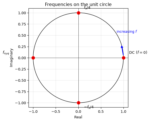
The fundamental interval is \(-f_\text{nyq} \leq f \leq f_\text{nyq}\), or equivalently \(-\pi \leq \phi \leq \pi\). Frequencies above \(f_\text{nyq}\) are aliases; they wrap back into this interval. This is the same aliasing from Chapter 1, now visible as periodicity on the unit circle.
fig, ax = plt.subplots(figsize=(5.5, 5.5))theta = np.linspace(0, 2* np.pi, 200)ax.plot(np.cos(theta), np.sin(theta), 'k-', linewidth=1)# Mark key pointspoints = [(1, 0, 'DC ($f=0$)'), (0, 1, '$f_s/4$'), (-1, 0, '$f_{nyq}$'), (0, -1, '$-f_s/4$')]for x, y, label in points: ax.plot(x, y, 'ro', markersize=8) offset = (15if x >=0else-80, 10if y >=0else-15) ax.annotate(label, (x, y), textcoords='offset points', xytext=offset, fontsize=10)# Arrow showing directionax.annotate('', xy=(np.cos(0.3), np.sin(0.3)), xytext=(np.cos(0.05), np.sin(0.05)), arrowprops=dict(arrowstyle='->', color='blue', lw=2))ax.text(0.85, 0.55, 'increasing $f$', color='blue', fontsize=9)ax.axhline(0, color='k', linewidth=0.5)ax.axvline(0, color='k', linewidth=0.5)ax.set_xlabel('Real')ax.set_ylabel('Imaginary')ax.set_aspect('equal')ax.set_title('Frequencies on the unit circle')ax.grid(True, alpha=0.3)fig.tight_layout()plt.show()
Figure 1: The unit circle as the frequency axis. Counterclockwise rotation from z=1 (DC) to z=−1 (Nyquist) covers all unique frequencies.
Frequency response of a filter
The frequency response\(H(e^{j\omega T})\) is the transfer function \(H(z)\) evaluated on the unit circle. It is a complex-valued function that tells you, for each frequency, how much the filter amplifies (magnitude) and shifts (phase) that frequency component.
The magnitude response\(|H(e^{j\omega T})|\) shows gain vs frequency. The phase response\(\angle H(e^{j\omega T})\) shows the phase shift. Together they form the Bode plot.
Computing with freqz
SciPy’s freqz computes the frequency response numerically, with no manual substitution needed:
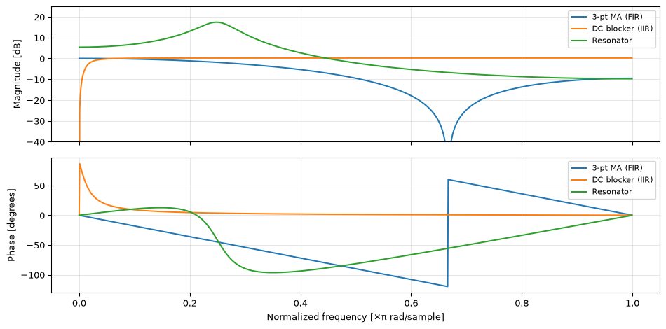
fig, axes = plt.subplots(2, 1, figsize=(10, 5), sharex=True)filters = {'3-pt MA (FIR)': ([1/3, 1/3, 1/3], [1]),'DC blocker (IIR)': ([1, -1], [1, -0.95]),'Resonator': ([1], [1, -2*0.9*np.cos(np.pi/4), 0.9**2]),}for name, (b, a) in filters.items(): w, H = freqz(b, a, worN=1024) freq_norm = w / np.pi # normalized to Nyquist mag_db =20* np.log10(np.maximum(np.abs(H), 1e-10)) phase_deg = np.degrees(np.unwrap(np.angle(H))) axes[0].plot(freq_norm, mag_db, linewidth=1.5, label=name) axes[1].plot(freq_norm, phase_deg, linewidth=1.5, label=name)axes[0].set_ylabel('Magnitude [dB]')axes[0].set_ylim(-40, 25)axes[0].legend(fontsize=8)axes[0].grid(True, alpha=0.3)axes[1].set_ylabel('Phase [degrees]')axes[1].set_xlabel('Normalized frequency [×π rad/sample]')axes[1].legend(fontsize=8)axes[1].grid(True, alpha=0.3)fig.tight_layout()plt.show()
Figure 2: Frequency response (Bode plot) of three filters from previous chapters. Top: magnitude in dB. Bottom: phase.
The MA filter is a lowpass (passes DC, attenuates high frequencies). The DC blocker is a highpass (zero at DC, passes high frequencies). The resonator has a sharp peak at \(\omega_0 = \pi/4\), exactly where its poles sit near the unit circle.
Magnitude from pole-zero geometry
There is an intuitive graphical interpretation: at each frequency \(\omega\), the magnitude is proportional to the product of distances from that point on the unit circle to each zero, divided by the product of distances to each pole:
\[|H(e^{j\omega T})| = K \cdot \frac{\prod \text{distances to zeros}}{\prod \text{distances to poles}}\]
When the unit circle passes close to a pole, the denominator becomes small and the magnitude peaks (resonance). When it passes through a zero, the magnitude drops to zero (notch).
Exercise: Reading the Bode plot
From the Bode plot above, estimate:
The DC gain of the 3-point MA filter (in dB and as a linear ratio).
The frequency at which the resonator peaks, in terms of normalized frequency.
Whether the DC blocker has finite or zero gain at DC.
Answer
The MA filter has 0 dB gain at DC, meaning a linear gain of 1.0. This makes sense: the coefficients \([1/3, 1/3, 1/3]\) sum to 1.
The resonator peaks at approximately \(0.25 \times \pi\) rad/sample, i.e. \(\omega_0 = \pi/4\), matching the pole angle.
The DC blocker has \(-\infty\) dB at DC (zero gain). The zero at \(z = 1\) forces \(H(e^{j0}) = 0\).
DTFT properties that matter
The DTFT obeys a set of properties that explain why many spectral phenomena occur. Not all properties are equally important in practice; the four below have direct consequences you’ll encounter often when working with real signals.
Property table
Property
Time domain
Frequency domain
Linearity
\(a\,x[n] + b\,y[n]\)
\(a\,X(e^{j\omega T}) + b\,Y(e^{j\omega T})\)
Time shift
\(x[n - d]\)
\(e^{-j\omega d T}\,X(e^{j\omega T})\)
Multiplication
\(x[n] \cdot w[n]\)
\(\frac{1}{2\pi} X \circledast W\) (periodic convolution in frequency)
The magnitude spectrum is symmetric about DC, which is why the single-sided spectrum contains all the information.
Why these matter
Time shift → phase rotation. Delaying a signal by \(d\) samples multiplies each frequency component by \(e^{-j\omega d T}\), a pure phase shift that increases linearly with frequency. This is why a delayed signal has a linear phase slope in the spectrum, and why a filter with constant group delay preserves waveform shapes (see Chapter 6).
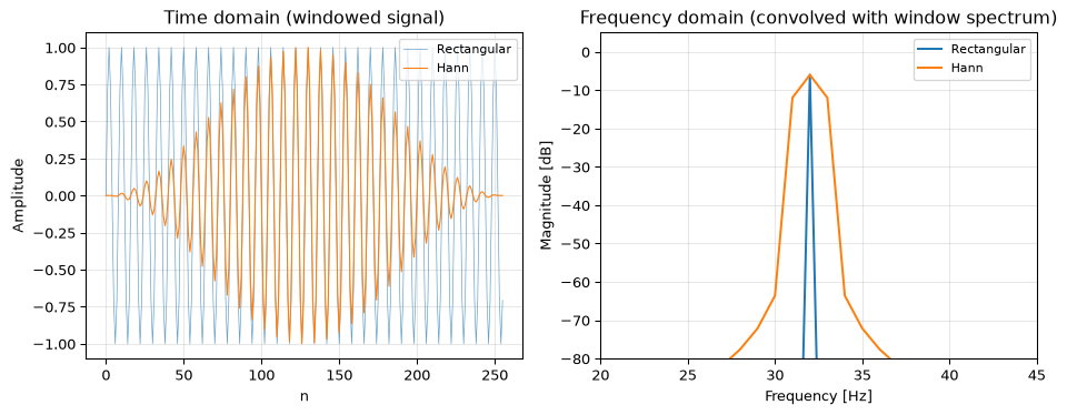
Multiplication → convolution in frequency (windowing and leakage). When you window a signal (multiply by \(w[n]\) in time), the spectrum is convolved with the window’s spectrum \(W\). The window’s main lobe width determines the frequency resolution; its side lobes determine the leakage. This is the precise explanation for the leakage phenomenon we’ll see later in this chapter: windowing smears every spectral peak by the shape of \(W\).
N =256fs =256n = np.arange(N)x = np.sin(2* np.pi *32* n / fs) # exact bin frequency# Rectangular (no window) vs Hann windowfrom scipy.signal import windowsw_rect = np.ones(N)w_hann = windows.hann(N)fig, axes = plt.subplots(1, 2, figsize=(10, 4))for w, name, color in [(w_rect, 'Rectangular', 'C0'), (w_hann, 'Hann', 'C1')]: xw = x * w X = np.fft.rfft(xw) freqs = np.fft.rfftfreq(N, 1/fs) mag_db =20* np.log10(np.maximum(np.abs(X) / np.sum(w), 1e-10)) axes[1].plot(freqs, mag_db, color=color, linewidth=1.5, label=name)axes[0].plot(n, x * w_rect, 'C0-', linewidth=0.5, alpha=0.7, label='Rectangular')axes[0].plot(n, x * w_hann, 'C1-', linewidth=0.8, label='Hann')axes[0].set_xlabel('n')axes[0].set_ylabel('Amplitude')axes[0].set_title('Time domain (windowed signal)')axes[0].legend(fontsize=8)axes[0].grid(True, alpha=0.3)axes[1].set_xlim(20, 45)axes[1].set_ylim(-80, 5)axes[1].set_xlabel('Frequency [Hz]')axes[1].set_ylabel('Magnitude [dB]')axes[1].set_title('Frequency domain (convolved with window spectrum)')axes[1].legend(fontsize=8)axes[1].grid(True, alpha=0.3)fig.tight_layout()plt.show()
Figure 3: Multiplication in time = convolution in frequency. Windowing a pure tone (left) smears its spectral line by the window’s frequency response (right).
Convolution → multiplication in frequency. Filtering in the time domain (convolution) becomes multiplication in the frequency domain. This is why we can analyse a filter’s effect by looking at its frequency response \(H(e^{j\omega T})\), and it’s the basis for FFT-based fast convolution (overlap-add).
The Discrete Fourier Transform (DFT)
The DTFT is continuous in frequency, so you can’t store it in a computer. The Discrete Fourier Transform (DFT) samples the DTFT at \(N\) equally-spaced frequencies, producing \(N\) complex coefficients from \(N\) input samples:
Each coefficient \(X_k\) represents the signal’s content at frequency \(f_k = k\,f_s / N\). The frequency spacing, called the frequency resolution, is \(\Delta f = f_s / N\).
No information is lost; you can go back and forth between time and frequency.
The FFT
The DFT requires \(O(N^2)\) operations. The Fast Fourier Transform (FFT) computes the same result in \(O(N \log N)\), a dramatic speedup. For \(N = 10^6\), that’s the difference between \(10^{12}\) and \(2 \times 10^7\) operations. The FFT is what makes real-time spectral analysis practical.
In Python, np.fft.fft computes the FFT. The result has \(N\) complex values; for real signals, the spectrum is symmetric, so only the first \(N/2 + 1\) values are unique (the single-sided spectrum).
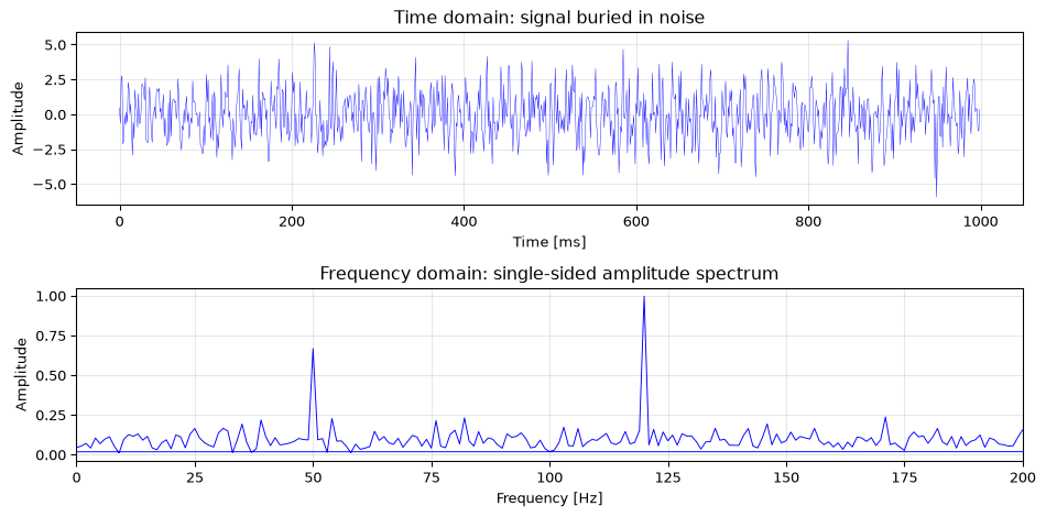
rng = np.random.default_rng(42)fs =1000# sampling frequencyT =1/fsN =1000# number of samplest = np.arange(N) * T# Signal: two sinusoids + noisesignal =0.7* np.sin(2*np.pi*50*t) + np.sin(2*np.pi*120*t)x = signal +1.5* rng.standard_normal(N)# Compute FFTX = np.fft.fft(x)freqs = np.fft.fftfreq(N, T)# Single-sided spectrum (DC and Nyquist are not doubled)n_half = N //2+1amp =2* np.abs(X[:n_half]) / Namp[0] /=2amp[-1] /=2fig, (ax1, ax2) = plt.subplots(2, 1, figsize=(10, 5))ax1.plot(t *1000, x, 'b-', linewidth=0.3)ax1.set_xlabel('Time [ms]')ax1.set_ylabel('Amplitude')ax1.set_title('Time domain: signal buried in noise')ax1.grid(True, alpha=0.3)ax2.plot(freqs[:n_half], amp, 'b-', linewidth=0.7)ax2.set_xlabel('Frequency [Hz]')ax2.set_ylabel('Amplitude')ax2.set_title('Frequency domain: single-sided amplitude spectrum')ax2.set_xlim(0, 200)ax2.grid(True, alpha=0.3)fig.tight_layout()plt.show()
Figure 4: FFT of a signal containing two sinusoids (50 Hz and 120 Hz) buried in noise. The frequency-domain representation reveals both components clearly.
The two sinusoids are invisible in the time domain but jump out immediately in the frequency domain. This is the power of spectral analysis.
Frequency resolution and zero-padding
The frequency resolution \(\Delta f = f_s / N\) depends on how many samples you have. More samples → finer resolution. If you need to resolve two tones separated by 5 Hz, you need at least \(N = f_s / 5\) samples.
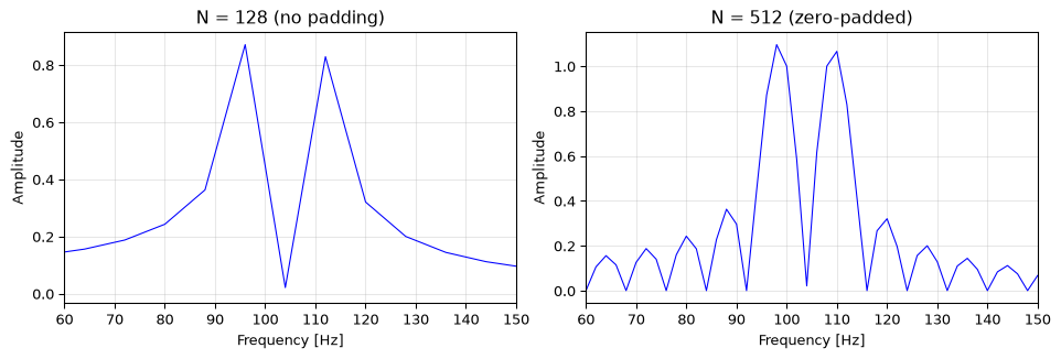
Zero-padding (appending zeros to the signal before the FFT) increases the number of frequency bins but does not improve the true resolution. It interpolates between existing DFT bins, making the spectrum look smoother, but it cannot reveal detail that isn’t in the original data.
fs =1024N =128t = np.arange(N) / fsx = np.sin(2*np.pi*100*t) + np.sin(2*np.pi*108*t)fig, axes = plt.subplots(1, 2, figsize=(10, 3.5))for ax, nfft, title inzip(axes, [N, 4*N], [f'N = {N} (no padding)', f'N = {4*N} (zero-padded)']): X = np.fft.fft(x, n=nfft) freqs = np.fft.fftfreq(nfft, 1/fs) n_half = nfft //2 amp =2* np.abs(X[:n_half]) / N # normalize by original N ax.plot(freqs[:n_half], amp, 'b-', linewidth=0.8) ax.set_xlim(60, 150) ax.set_xlabel('Frequency [Hz]') ax.set_ylabel('Amplitude') ax.set_title(title) ax.grid(True, alpha=0.3)fig.tight_layout()plt.show()
Figure 5: Zero-padding interpolates the spectrum but does not improve resolution. Both plots show two tones at 100 and 108 Hz, barely resolvable with N=128 at fs=1024 Hz (Δf = 8 Hz).
Exercise: Frequency resolution
You sample a signal at \(f_s = 8000\) Hz and want to distinguish two tones 10 Hz apart. What is the minimum number of samples needed? How long a recording is that?
Answer
\(\Delta f = f_s / N \leq 10\) Hz, so \(N \geq 800\) samples. At \(f_s = 8000\) Hz, that’s \(800/8000 = 0.1\) seconds of data.
Practical FFT usage
The DFT math is clean, but getting a correctly-scaled, correctly-labelled spectrum from real data is a common stumbling block. This section covers the practical details.
fft vs rfft for real signals
Real-valued signals have conjugate-symmetric spectra: \(X[k] = X^*[N-k]\). This means the negative-frequency half is redundant. Use np.fft.rfft instead of np.fft.fft: it returns only the \(N/2 + 1\) unique bins, runs faster, and uses less memory:
N =1024x = np.random.default_rng(42).standard_normal(N)X_full = np.fft.fft(x) # N complex values (redundant for real x)X_half = np.fft.rfft(x) # N/2+1 complex values (all unique)print(f"fft output: {X_full.shape[0]} bins")print(f"rfft output: {X_half.shape[0]} bins")print(f"Match: {np.allclose(X_full[:N//2+1], X_half)}")
This is one of the most common sources of FFT bugs. The rules:
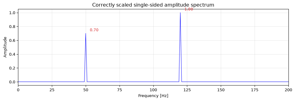
Amplitude spectrum (peak height matches sinusoid amplitude): divide by \(N\), then multiply by 2 for single-sided, but not for the DC bin (\(k=0\)) or the Nyquist bin (\(k=N/2\)), since those don’t have a mirror image.
Power spectral density (power per Hz): \(|X_k|^2 / (N \cdot f_s)\), doubled for single-sided interior bins.
Figure 6: Correct amplitude scaling: the FFT recovers the true amplitudes (0.7 and 1.0) of the two sinusoids.
FFT speed: fast lengths
The FFT is fastest for lengths that are products of small primes (2, 3, 5). Use scipy.fft.next_fast_len to pad to an efficient size:
from scipy.fft import next_fast_lenfor N in [1000, 1023, 1024, 4000, 4096]: fast_N = next_fast_len(N)print(f"N = {N:5d} → fast length = {fast_N:5d}{'(already fast)'if N == fast_N else''}")
N =  1000 → fast length =  1000  (already fast)
N =  1023 → fast length =  1024
N =  1024 → fast length =  1024  (already fast)
N =  4000 → fast length =  4000  (already fast)
N =  4096 → fast length =  4096  (already fast)
FFT-based convolution
For long signals, convolution via the FFT is faster than direct convolution. The crossover is typically around 50–100 taps, depending on the implementation and FFT size. scipy.signal.fftconvolve handles this automatically, including the case where the signal is much longer than the filter (it uses overlap-add internally):
from scipy.signal import fftconvolve, firwin# A long signal filtered with a 101-tap FIRfs =8000x = np.random.default_rng(42).standard_normal(100_000)h = firwin(101, 1000, fs=fs)# Direct convolution vs FFT convolution — same resulty_direct = np.convolve(x, h, mode='same')y_fft = fftconvolve(x, h, mode='same')print(f"Max difference: {np.max(np.abs(y_direct - y_fft)):.2e}")
Max difference: 1.55e-15
For very long signals (millions of samples), scipy.signal.oaconvolve (overlap-add) is even faster because it processes the signal in blocks without needing a single FFT the length of the entire signal.
Recipe: spectrum of a real signal
Here is the complete pattern for computing a correctly-scaled, correctly-labelled spectrum:
def amplitude_spectrum(x, fs):"""Single-sided amplitude spectrum of a real signal.""" N =len(x) X = np.fft.rfft(x) freqs = np.fft.rfftfreq(N, 1/fs) amp = np.abs(X) / N amp[1:-1] *=2# single-sided (don't double DC or Nyquist)return freqs, amp
Parseval’s theorem
Parseval’s theorem (Proakis and Manolakis 2007) states that the total energy of a signal is the same whether you compute it in the time domain or the frequency domain:
In words: the sum of squared magnitudes in time equals the (scaled) sum of squared magnitudes in frequency. No energy is created or destroyed by the DFT; it just redistributes it across frequency bins.
This is more than an elegant identity. It has practical consequences:
Checking implementations: if your time-domain energy and frequency-domain energy disagree, there’s a bug.
Filtering: removing frequency bins removes exactly that much energy from the signal.
Noise floor: the total noise power you see in a spectrum must equal the noise power measured in the time domain.
The factor of \(1/N\) comes from the DFT normalization convention. NumPy uses the convention where the forward DFT has no scaling and the inverse DFT divides by \(N\). If you use a different convention (e.g., \(1/\sqrt{N}\) on both transforms), Parseval’s theorem has no extra factor.
Spectral leakage and windowing
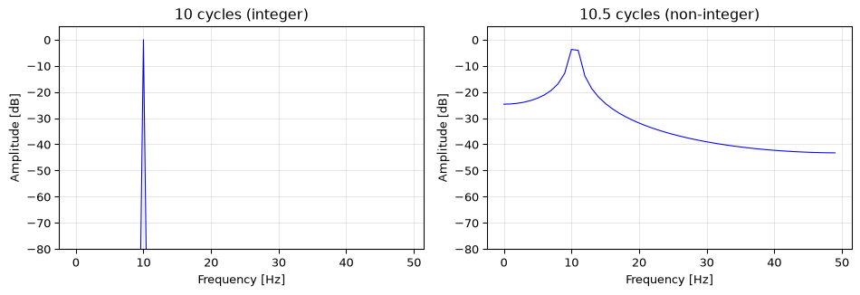
The DFT assumes the input is periodic with period \(N\). When the signal does not contain an integer number of cycles in the analysis window, the endpoints don’t match up, creating artificial discontinuities. These discontinuities spread energy across all frequency bins, an artifact called spectral leakage.
Figure 8: Spectral leakage: a pure 10 Hz tone analysed with exactly 10 cycles (left, no leakage) vs 10.5 cycles (right, energy leaks across bins).
Window functions
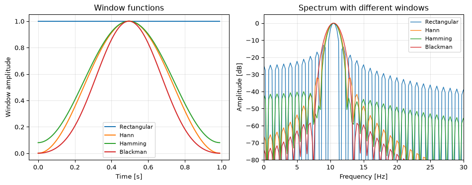
A window function tapers the signal smoothly to zero at both ends, reducing the discontinuity and thus the leakage. The trade-off: windows widen the main lobe (reducing resolution) but suppress the side lobes (reducing leakage).
Figure 9: Effect of window functions on a 10.5 Hz tone. Windowing reduces side lobes (leakage) at the cost of a wider main lobe.
The rectangular window (no windowing) has the narrowest peak but leakage down to only −13 dB. The Hann window widens the peak slightly but pushes side lobes below −31 dB. For most spectral analysis work, Hann is the default choice.
Exercise: Choosing a window
You need to detect a weak signal at 105 Hz in the presence of a strong signal at 100 Hz. The weak signal is 40 dB below the strong one. Which window function from the table above would you choose, and why?
Answer
You need side lobes below −40 dB so the strong signal’s leakage doesn’t mask the weak one. The Hamming window (−43 dB side lobes) is the minimum; Blackman (−58 dB) gives more margin. The rectangular window (−13 dB) would completely mask the weak signal.
Power spectral density estimation
In practice, you often want to estimate how a signal’s power is distributed across frequencies: the power spectral density (PSD). This connects directly to the noise analysis in Chapter 3: white noise has a flat PSD, pink noise falls as \(1/f\), and filtering reshapes the PSD.
The periodogram
The simplest PSD estimate squares the FFT magnitude:
\[\hat{S}(f_k) = \frac{1}{N\,f_s} |X_k|^2\]
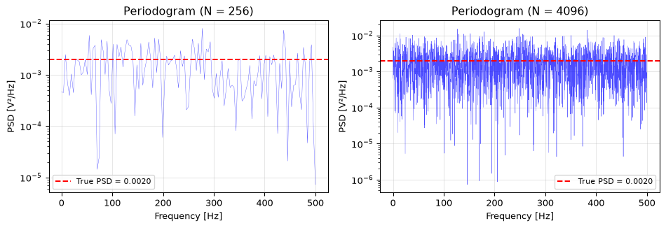
This is the periodogram. It is unbiased but has high variance; it’s noisy, even for long signals. Doubling the signal length does not smooth the periodogram; it just adds more noisy frequency bins.
The trade-off: each segment is shorter than the full signal, so frequency resolution decreases. But the averaging dramatically reduces the variance, and the PSD estimate becomes smooth and reliable.
rng = np.random.default_rng(42)fs =1000N =4096x = rng.standard_normal(N)# Raw periodogramfreqs_raw = np.fft.rfftfreq(N, 1/fs)X = np.fft.rfft(x)psd_raw = np.abs(X)**2/ (N * fs)psd_raw[1:-1] *=2# one-sided: double all except DC and Nyquist# Welch with different segment lengthsfig, ax = plt.subplots(figsize=(10, 4))ax.semilogy(freqs_raw, psd_raw, 'b-', linewidth=0.3, alpha=0.4, label='Periodogram')for nperseg, color in [(256, 'C1'), (512, 'C2')]: f_welch, psd_welch = welch(x, fs, nperseg=nperseg) ax.semilogy(f_welch, psd_welch, color, linewidth=1.5, label=f'Welch (nperseg={nperseg})')ax.axhline(2/fs, color='r', linewidth=1, linestyle='--', label='True PSD')ax.set_xlabel('Frequency [Hz]')ax.set_ylabel('PSD [V²/Hz]')ax.set_title("Welch's method vs periodogram")ax.legend(fontsize=8)ax.grid(True, alpha=0.3)fig.tight_layout()plt.show()
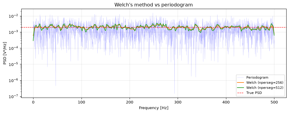
Figure 11: Welch’s method vs the raw periodogram. Welch averages over segments, producing a much smoother PSD estimate.
scipy.signal.welch does all of this in one call. The key parameter is nperseg, the segment length. Shorter segments give smoother estimates but coarser frequency resolution.
The resolution–variance trade-off
This is a fundamental tension in spectral estimation: you cannot simultaneously have high frequency resolution and low variance. Long windows give fine resolution but noisy estimates; short windows (more averages) give smooth estimates but coarse resolution. There is no free lunch; you must choose based on what matters for your application.
Practical example: identifying noise type
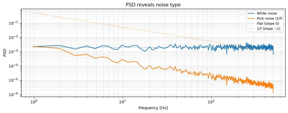
In Chapter 3, we saw that white noise has a flat PSD and pink noise falls as \(1/f\). Welch’s method lets you verify this from data:
Figure 12: PSD estimation with Welch’s method identifies the noise type from its spectral slope.
Exercise: Welch parameters
You have a 10-second recording sampled at \(f_s = 44100\) Hz. You want to estimate the PSD with a frequency resolution of at least 5 Hz.
What is the minimum segment length (nperseg) for Welch’s method?
With 50% overlap, approximately how many segments will be averaged?
Answer
\(\Delta f = f_s / N_\text{seg} \leq 5\) Hz, so \(N_\text{seg} \geq 44100/5 = 8820\) samples. Round up to a power of 2 for FFT efficiency: nperseg = 16384 (giving \(\Delta f \approx 2.7\) Hz).
Total samples = \(44100 \times 10 = 441000\). With 50% overlap, each new segment advances by \(N_\text{seg}/2 = 8192\) samples, so the count is \(\lfloor (441000 - 16384)/8192 \rfloor + 1 \approx 52\). More averages → smoother PSD estimate.
The Wiener–Khinchin theorem
In Chapter 3 we introduced the autocorrelation \(R_{xx}[k]\) as a measure of how a signal correlates with itself at different lags. The power spectral density (PSD) describes how power is distributed across frequencies. The Wiener–Khinchin theorem connects the two:
\[S_{xx}(f) = \mathcal{F}\{R_{xx}[k]\}\]
The PSD is the Fourier transform of the autocorrelation function (Papoulis and Pillai 2002). Equivalently, the autocorrelation is the inverse Fourier transform of the PSD:
\[R_{xx}[k] = \mathcal{F}^{-1}\{S_{xx}(f)\}\]
This relationship makes intuitive sense: autocorrelation captures periodic structure in a signal (positive correlations at regular lags), and the Fourier transform converts that periodic structure into frequency peaks. White noise has \(R_{xx}[k] = \sigma^2\,\delta[k]\), whose Fourier transform is a constant, a flat PSD, exactly as expected.
Let’s verify this numerically, computing the PSD two different ways:
rng = np.random.default_rng(42)N =2048fs =1000# Colored noise (AR process)white = rng.standard_normal(N)from scipy.signal import lfilterx = lfilter([1], [1, -0.85], white)# Method 1: Periodogram (|X|^2 / (N*fs))X = np.fft.rfft(x)freqs = np.fft.rfftfreq(N, 1/fs)psd_periodogram = np.abs(X)**2/ (N * fs)psd_periodogram[1:-1] *=2# single-sided# Method 2: DFT of autocorrelationr_full = np.correlate(x, x, mode='full') / N # biased estimateR = r_full[N-1:] # keep non-negative lags# Take DFT of full symmetric autocorrelation (zero-pad to N for matching freq grid)r_symmetric = np.zeros(N)r_symmetric[:len(R)] = R # lags 0..N-1r_symmetric[-(len(R)-1):] = R[1:][::-1] # mirror negative lagsS_from_acf = np.real(np.fft.rfft(r_symmetric)) / fs # real for symmetric inputS_from_acf[1:-1] *=2# single-sidedfig, ax = plt.subplots(figsize=(10, 4))ax.semilogy(freqs, psd_periodogram, 'C0-', linewidth=0.5, alpha=0.6, label='Periodogram $|X|^2/(Nf_s)$')ax.semilogy(freqs, S_from_acf, 'C1-', linewidth=1.5, alpha=0.8, label='DFT of $R_{xx}[k]$')ax.set_xlabel('Frequency [Hz]')ax.set_ylabel('PSD')ax.set_title('Wiener–Khinchin: two routes to the same PSD')ax.legend(fontsize=9)ax.grid(True, alpha=0.3, which='both')fig.tight_layout()plt.show()
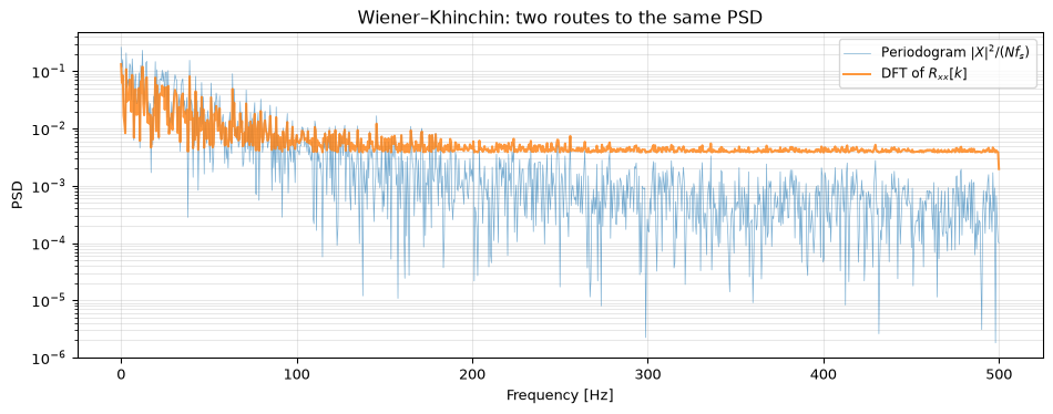
Figure 13: The Wiener–Khinchin theorem verified: PSD computed via the periodogram and via the DFT of the autocorrelation function give the same result.
The two curves lie on top of each other; the periodogram is the DFT of the autocorrelation, just computed differently. Welch’s method (above) smooths this estimate by averaging over segments.
The spectrogram
So far, spectral analysis assumes the signal is stationary, meaning its frequency content doesn’t change over time. But many real signals are non-stationary: speech, music, chirps, engine vibrations.
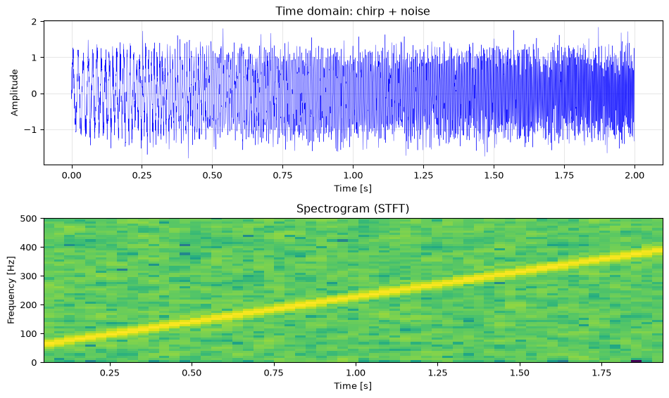
The spectrogram handles this by computing the spectrum in short, overlapping windows that slide along the signal, using the Short-Time Fourier Transform (STFT). The result is a time-frequency map showing how the spectrum evolves.
Figure 14: Spectrogram of a chirp signal sweeping from 50 to 400 Hz. The time-frequency representation tracks the instantaneous frequency.
The spectrogram reveals the linear frequency sweep that is invisible in the time-domain waveform. The window length (NFFT) controls the resolution trade-off: short windows give good time resolution but poor frequency resolution; long windows give the opposite.
The uncertainty principle
The time-frequency resolution trade-off is not a limitation of the algorithm; it’s a fundamental property of signals. A signal cannot be simultaneously localised in both time and frequency. This is the Gabor limit(Gabor 1946), the signal-processing analogue of Heisenberg’s uncertainty principle. For the STFT, a practical form is: \(\Delta t \cdot \Delta f \geq 1\), where \(\Delta t\) is the window duration and \(\Delta f = 1/\Delta t\) is the frequency resolution (\(\Delta t \cdot \Delta f \geq 1\) using the time-bandwidth product convention; the Heisenberg–Gabor bound \(\Delta t \cdot \Delta f \geq 1/(4\pi)\) uses RMS widths of the squared envelope). The signal that reaches this bound is the Gaussian-windowed sinusoid, or Gabor atom; its 2-D form is the oriented receptive field of the visual cortex, explored in the Gabor filters topic.
Summary
Concept
Key result
DTFT
\(X(e^{j\omega T}) = \sum x[n]\,e^{-j\omega nT}\), the z-transform on the unit circle
Frequency response
\(H(e^{j\omega T})\): magnitude and phase vs frequency
Unit circle
DC at \(z=1\), Nyquist at \(z=-1\), fundamental interval \([-\pi, \pi]\)
DFT / FFT
\(N\) samples → \(N\) frequency bins, resolution \(\Delta f = f_s/N\)
Parseval’s theorem
\(\sum|x[n]|^2 = \frac{1}{N}\sum|X_k|^2\): energy is conserved
Windowing
Reduces spectral leakage at the cost of wider main lobe
Periodogram
\(|X_k|^2/(Nf_s)\): unbiased but high variance
Welch’s method
Segment + window + average: smooth PSD estimate
Wiener–Khinchin
\(S_{xx}(f) = \mathcal{F}\{R_{xx}[k]\}\): PSD is the DFT of autocorrelation
Spectrogram
STFT: time-frequency representation for non-stationary signals
This chapter completes the core signal analysis framework: time domain (Chapters 1–2), z-domain (Chapter 4), and now the frequency domain. The next chapter applies these tools to the design of digital filters: Filter design.
Proakis & Manolakis, Digital Signal Processing (2007), Ch. 5: DFT, Ch. 12.3: Welch’s method
Going deeper
Several Topics pages use frequency-domain tools from this chapter:
Noise whitening: estimating the spectral exponent of colored noise and flattening the PSD
Adaptive filtering: real-time filters that converge in the frequency domain
Matched filtering: optimal detection via cross-correlation (frequency-domain implementation)
References
Gabor, Dennis. 1946. “Theory of Communication.”Journal of the Institution of Electrical Engineers 93 (26): 429–57.
Oppenheim, Alan V., and Ronald W. Schafer. 2010. Discrete-Time Signal Processing. 3rd ed. Pearson.
Papoulis, Athanasios, and S. Unnikrishna Pillai. 2002. Probability, Random Variables, and Stochastic Processes. 4th ed. McGraw-Hill.
Proakis, John G., and Dimitris G. Manolakis. 2007. Digital Signal Processing: Principles, Algorithms, and Applications. 4th ed. Pearson.
Source Code
---title: "The Frequency Domain"subtitle: "Frequency response, DFT, FFT, and spectral estimation"---```{python}#| echo: falseimport numpy as npimport matplotlib.pyplot as pltfrom scipy.signal import freqz, welch```So far we have described signals and filters entirely in the time domain (Chapters 1–2) or as polynomials in $z$ (Chapter 4). But many real-world questions are naturally about **frequency**: *What tones are in this recording? Where does my sensor's noise live? Does this filter pass 50 Hz or block it?*The frequency domain answers these questions directly. This chapter builds the bridge from the z-transform to frequencies, introduces the DFT and FFT for practical computation, and ends with **spectral density estimation**: the tools you actually use to analyse real signals.---## From z-domain to frequency domainIn [Chapter 4](04-z-domain.qmd), we defined $z = A\,e^{j\phi}$. On the **unit circle**, $A = 1$, so $z = e^{j\phi}$. Substituting $\phi = \omega T$ (where $\omega$ is angular frequency in rad/s and $T = 1/f_s$ is the sampling period):$$z = e^{j\omega T}$$Evaluating the z-transform on the unit circle gives the **discrete-time Fourier transform** (DTFT) [@oppenheim2010discrete]:$$X(e^{j\omega T}) = \sum_{n=-\infty}^{\infty} x[n]\,e^{-j\omega n T}$$This is a continuous, periodic function of frequency with period $f_s$. It maps each point on the unit circle to a complex number encoding the amplitude and phase at that frequency.### The unit circle as the frequency axisWalking counterclockwise around the unit circle sweeps through all frequencies:| Point on unit circle | Angle $\phi$ | Frequency ||---------------------|--------------|-----------|| $z = 1$ | $0$ | $0$ (DC) || $z = j$ | $\pi/2$ | $f_s/4$ || $z = -1$ | $\pi$ | $f_s/2 = f_\text{nyq}$ || $z = -j$ | $3\pi/2$ (or $-\pi/2$) | $3f_s/4$ (or $-f_s/4$) || $z = 1$ | $2\pi$ | $f_s$ (= DC again) |The **fundamental interval** is $-f_\text{nyq} \leq f \leq f_\text{nyq}$, or equivalently $-\pi \leq \phi \leq \pi$. Frequencies above $f_\text{nyq}$ are aliases; they wrap back into this interval. This is the same aliasing from [Chapter 1](01-signals.qmd), now visible as periodicity on the unit circle.```{python}#| label: fig-unit-circle-freq#| fig-cap: "The unit circle as the frequency axis. Counterclockwise rotation from z=1 (DC) to z=−1 (Nyquist) covers all unique frequencies."fig, ax = plt.subplots(figsize=(5.5, 5.5))theta = np.linspace(0, 2* np.pi, 200)ax.plot(np.cos(theta), np.sin(theta), 'k-', linewidth=1)# Mark key pointspoints = [(1, 0, 'DC ($f=0$)'), (0, 1, '$f_s/4$'), (-1, 0, '$f_{nyq}$'), (0, -1, '$-f_s/4$')]for x, y, label in points: ax.plot(x, y, 'ro', markersize=8) offset = (15if x >=0else-80, 10if y >=0else-15) ax.annotate(label, (x, y), textcoords='offset points', xytext=offset, fontsize=10)# Arrow showing directionax.annotate('', xy=(np.cos(0.3), np.sin(0.3)), xytext=(np.cos(0.05), np.sin(0.05)), arrowprops=dict(arrowstyle='->', color='blue', lw=2))ax.text(0.85, 0.55, 'increasing $f$', color='blue', fontsize=9)ax.axhline(0, color='k', linewidth=0.5)ax.axvline(0, color='k', linewidth=0.5)ax.set_xlabel('Real')ax.set_ylabel('Imaginary')ax.set_aspect('equal')ax.set_title('Frequencies on the unit circle')ax.grid(True, alpha=0.3)fig.tight_layout()plt.show()```---## Frequency response of a filterThe **frequency response** $H(e^{j\omega T})$ is the transfer function $H(z)$ evaluated on the unit circle. It is a complex-valued function that tells you, for each frequency, how much the filter amplifies (magnitude) and shifts (phase) that frequency component.$$H(e^{j\omega T}) = H(z)\big|_{z=e^{j\omega T}}$$The **magnitude response** $|H(e^{j\omega T})|$ shows gain vs frequency. The **phase response** $\angle H(e^{j\omega T})$ shows the phase shift. Together they form the **Bode plot**.### Computing with `freqz`SciPy's `freqz` computes the frequency response numerically, with no manual substitution needed:```{python}#| label: fig-freqz-demo#| fig-cap: "Frequency response (Bode plot) of three filters from previous chapters. Top: magnitude in dB. Bottom: phase."fig, axes = plt.subplots(2, 1, figsize=(10, 5), sharex=True)filters = {'3-pt MA (FIR)': ([1/3, 1/3, 1/3], [1]),'DC blocker (IIR)': ([1, -1], [1, -0.95]),'Resonator': ([1], [1, -2*0.9*np.cos(np.pi/4), 0.9**2]),}for name, (b, a) in filters.items(): w, H = freqz(b, a, worN=1024) freq_norm = w / np.pi # normalized to Nyquist mag_db =20* np.log10(np.maximum(np.abs(H), 1e-10)) phase_deg = np.degrees(np.unwrap(np.angle(H))) axes[0].plot(freq_norm, mag_db, linewidth=1.5, label=name) axes[1].plot(freq_norm, phase_deg, linewidth=1.5, label=name)axes[0].set_ylabel('Magnitude [dB]')axes[0].set_ylim(-40, 25)axes[0].legend(fontsize=8)axes[0].grid(True, alpha=0.3)axes[1].set_ylabel('Phase [degrees]')axes[1].set_xlabel('Normalized frequency [×π rad/sample]')axes[1].legend(fontsize=8)axes[1].grid(True, alpha=0.3)fig.tight_layout()plt.show()```The MA filter is a lowpass (passes DC, attenuates high frequencies). The DC blocker is a highpass (zero at DC, passes high frequencies). The resonator has a sharp peak at $\omega_0 = \pi/4$, exactly where its poles sit near the unit circle.### Magnitude from pole-zero geometryThere is an intuitive graphical interpretation: at each frequency $\omega$, the magnitude is proportional to the product of distances from that point on the unit circle to each **zero**, divided by the product of distances to each **pole**:$$|H(e^{j\omega T})| = K \cdot \frac{\prod \text{distances to zeros}}{\prod \text{distances to poles}}$$When the unit circle passes close to a pole, the denominator becomes small and the magnitude peaks (resonance). When it passes through a zero, the magnitude drops to zero (notch).::: {.callout-tip collapse="true" title="Exercise: Reading the Bode plot"}From the Bode plot above, estimate:a) The DC gain of the 3-point MA filter (in dB and as a linear ratio).b) The frequency at which the resonator peaks, in terms of normalized frequency.c) Whether the DC blocker has finite or zero gain at DC.::: {.callout-note collapse="true" title="Answer"}a) The MA filter has 0 dB gain at DC, meaning a linear gain of 1.0. This makes sense: the coefficients $[1/3, 1/3, 1/3]$ sum to 1.b) The resonator peaks at approximately $0.25 \times \pi$ rad/sample, i.e. $\omega_0 = \pi/4$, matching the pole angle.c) The DC blocker has $-\infty$ dB at DC (zero gain). The zero at $z = 1$ forces $H(e^{j0}) = 0$.::::::---## DTFT properties that matterThe DTFT obeys a set of properties that explain *why* many spectral phenomena occur. Not all properties are equally important in practice; the four below have direct consequences you'll encounter often when working with real signals.### Property table| Property | Time domain | Frequency domain ||----------|-------------|------------------|| **Linearity** | $a\,x[n] + b\,y[n]$ | $a\,X(e^{j\omega T}) + b\,Y(e^{j\omega T})$ || **Time shift** | $x[n - d]$ | $e^{-j\omega d T}\,X(e^{j\omega T})$ || **Multiplication** | $x[n] \cdot w[n]$ | $\frac{1}{2\pi} X \circledast W$ (periodic convolution in frequency) || **Convolution** | $x[n] * h[n]$ | $X(e^{j\omega T}) \cdot H(e^{j\omega T})$ |And one symmetry property for real signals:$$x[n] \in \mathbb{R} \implies X(e^{j\omega T}) = X^*(e^{-j\omega T})$$The magnitude spectrum is symmetric about DC, which is why the single-sided spectrum contains all the information.### Why these matter**Time shift → phase rotation.** Delaying a signal by $d$ samples multiplies each frequency component by $e^{-j\omega d T}$, a pure phase shift that increases linearly with frequency. This is why a delayed signal has a linear phase slope in the spectrum, and why a filter with constant group delay preserves waveform shapes (see [Chapter 6](06-filter-design.qmd)).**Multiplication → convolution in frequency (windowing and leakage).** When you window a signal (multiply by $w[n]$ in time), the spectrum is *convolved* with the window's spectrum $W$. The window's main lobe width determines the frequency resolution; its side lobes determine the leakage. This is the precise explanation for the leakage phenomenon we'll see later in this chapter: windowing smears every spectral peak by the shape of $W$.```{python}#| label: fig-windowing-duality#| fig-cap: "Multiplication in time = convolution in frequency. Windowing a pure tone (left) smears its spectral line by the window's frequency response (right)."N =256fs =256n = np.arange(N)x = np.sin(2* np.pi *32* n / fs) # exact bin frequency# Rectangular (no window) vs Hann windowfrom scipy.signal import windowsw_rect = np.ones(N)w_hann = windows.hann(N)fig, axes = plt.subplots(1, 2, figsize=(10, 4))for w, name, color in [(w_rect, 'Rectangular', 'C0'), (w_hann, 'Hann', 'C1')]: xw = x * w X = np.fft.rfft(xw) freqs = np.fft.rfftfreq(N, 1/fs) mag_db =20* np.log10(np.maximum(np.abs(X) / np.sum(w), 1e-10)) axes[1].plot(freqs, mag_db, color=color, linewidth=1.5, label=name)axes[0].plot(n, x * w_rect, 'C0-', linewidth=0.5, alpha=0.7, label='Rectangular')axes[0].plot(n, x * w_hann, 'C1-', linewidth=0.8, label='Hann')axes[0].set_xlabel('n')axes[0].set_ylabel('Amplitude')axes[0].set_title('Time domain (windowed signal)')axes[0].legend(fontsize=8)axes[0].grid(True, alpha=0.3)axes[1].set_xlim(20, 45)axes[1].set_ylim(-80, 5)axes[1].set_xlabel('Frequency [Hz]')axes[1].set_ylabel('Magnitude [dB]')axes[1].set_title('Frequency domain (convolved with window spectrum)')axes[1].legend(fontsize=8)axes[1].grid(True, alpha=0.3)fig.tight_layout()plt.show()```**Convolution → multiplication in frequency.** Filtering in the time domain (convolution) becomes multiplication in the frequency domain. This is why we can analyse a filter's effect by looking at its frequency response $H(e^{j\omega T})$, and it's the basis for FFT-based fast convolution (overlap-add).---## The Discrete Fourier Transform (DFT)The DTFT is continuous in frequency, so you can't store it in a computer. The **Discrete Fourier Transform** (DFT) samples the DTFT at $N$ equally-spaced frequencies, producing $N$ complex coefficients from $N$ input samples:$$X_k = \sum_{n=0}^{N-1} x[n]\,e^{-j2\pi kn/N}, \qquad k = 0, 1, \ldots, N-1$$Each coefficient $X_k$ represents the signal's content at frequency $f_k = k\,f_s / N$. The frequency spacing, called the **frequency resolution**, is $\Delta f = f_s / N$.The DFT is **invertible**:$$x[n] = \frac{1}{N}\sum_{k=0}^{N-1} X_k\,e^{+j2\pi kn/N}$$No information is lost; you can go back and forth between time and frequency.### The FFTThe DFT requires $O(N^2)$ operations. The **Fast Fourier Transform** (FFT) computes the same result in $O(N \log N)$, a dramatic speedup. For $N = 10^6$, that's the difference between $10^{12}$ and $2 \times 10^7$ operations. The FFT is what makes real-time spectral analysis practical.In Python, `np.fft.fft` computes the FFT. The result has $N$ complex values; for real signals, the spectrum is symmetric, so only the first $N/2 + 1$ values are unique (the **single-sided spectrum**).```{python}#| label: fig-fft-basic#| fig-cap: "FFT of a signal containing two sinusoids (50 Hz and 120 Hz) buried in noise. The frequency-domain representation reveals both components clearly."rng = np.random.default_rng(42)fs =1000# sampling frequencyT =1/fsN =1000# number of samplest = np.arange(N) * T# Signal: two sinusoids + noisesignal =0.7* np.sin(2*np.pi*50*t) + np.sin(2*np.pi*120*t)x = signal +1.5* rng.standard_normal(N)# Compute FFTX = np.fft.fft(x)freqs = np.fft.fftfreq(N, T)# Single-sided spectrum (DC and Nyquist are not doubled)n_half = N //2+1amp =2* np.abs(X[:n_half]) / Namp[0] /=2amp[-1] /=2fig, (ax1, ax2) = plt.subplots(2, 1, figsize=(10, 5))ax1.plot(t *1000, x, 'b-', linewidth=0.3)ax1.set_xlabel('Time [ms]')ax1.set_ylabel('Amplitude')ax1.set_title('Time domain: signal buried in noise')ax1.grid(True, alpha=0.3)ax2.plot(freqs[:n_half], amp, 'b-', linewidth=0.7)ax2.set_xlabel('Frequency [Hz]')ax2.set_ylabel('Amplitude')ax2.set_title('Frequency domain: single-sided amplitude spectrum')ax2.set_xlim(0, 200)ax2.grid(True, alpha=0.3)fig.tight_layout()plt.show()```The two sinusoids are invisible in the time domain but jump out immediately in the frequency domain. This is the power of spectral analysis.### Frequency resolution and zero-paddingThe frequency resolution $\Delta f = f_s / N$ depends on how many samples you have. More samples → finer resolution. If you need to resolve two tones separated by 5 Hz, you need at least $N = f_s / 5$ samples.**Zero-padding** (appending zeros to the signal before the FFT) increases the number of frequency bins but does **not** improve the true resolution. It interpolates between existing DFT bins, making the spectrum look smoother, but it cannot reveal detail that isn't in the original data.```{python}#| label: fig-zero-padding#| fig-cap: "Zero-padding interpolates the spectrum but does not improve resolution. Both plots show two tones at 100 and 108 Hz, barely resolvable with N=128 at fs=1024 Hz (Δf = 8 Hz)."fs =1024N =128t = np.arange(N) / fsx = np.sin(2*np.pi*100*t) + np.sin(2*np.pi*108*t)fig, axes = plt.subplots(1, 2, figsize=(10, 3.5))for ax, nfft, title inzip(axes, [N, 4*N], [f'N = {N} (no padding)', f'N = {4*N} (zero-padded)']): X = np.fft.fft(x, n=nfft) freqs = np.fft.fftfreq(nfft, 1/fs) n_half = nfft //2 amp =2* np.abs(X[:n_half]) / N # normalize by original N ax.plot(freqs[:n_half], amp, 'b-', linewidth=0.8) ax.set_xlim(60, 150) ax.set_xlabel('Frequency [Hz]') ax.set_ylabel('Amplitude') ax.set_title(title) ax.grid(True, alpha=0.3)fig.tight_layout()plt.show()```::: {.callout-tip collapse="true" title="Exercise: Frequency resolution"}You sample a signal at $f_s = 8000$ Hz and want to distinguish two tones 10 Hz apart. What is the minimum number of samples needed? How long a recording is that?::: {.callout-note collapse="true" title="Answer"}$\Delta f = f_s / N \leq 10$ Hz, so $N \geq 800$ samples. At $f_s = 8000$ Hz, that's $800/8000 = 0.1$ seconds of data.::::::---## Practical FFT usageThe DFT math is clean, but getting a correctly-scaled, correctly-labelled spectrum from real data is a common stumbling block. This section covers the practical details.### `fft` vs `rfft` for real signalsReal-valued signals have conjugate-symmetric spectra: $X[k] = X^*[N-k]$. This means the negative-frequency half is redundant. Use `np.fft.rfft` instead of `np.fft.fft`: it returns only the $N/2 + 1$ unique bins, runs faster, and uses less memory:```{python}N =1024x = np.random.default_rng(42).standard_normal(N)X_full = np.fft.fft(x) # N complex values (redundant for real x)X_half = np.fft.rfft(x) # N/2+1 complex values (all unique)print(f"fft output: {X_full.shape[0]} bins")print(f"rfft output: {X_half.shape[0]} bins")print(f"Match: {np.allclose(X_full[:N//2+1], X_half)}")```### Frequency axis constructionUse `rfftfreq` (not `fftfreq`) with `rfft`:```{python}fs =1000N =256freqs = np.fft.rfftfreq(N, d=1/fs) # d = sample spacing in secondsprint(f"Bin 0: {freqs[0]:.1f} Hz (DC)")print(f"Bin 1: {freqs[1]:.4f} Hz (= fs/N = {fs/N:.4f})")print(f"Last: {freqs[-1]:.1f} Hz (Nyquist = fs/2)")print(f"Δf: {freqs[1]-freqs[0]:.4f} Hz")```### Amplitude scalingThis is one of the most common sources of FFT bugs. The rules:- **Amplitude spectrum** (peak height matches sinusoid amplitude): divide by $N$, then multiply by 2 for single-sided, but **not** for the DC bin ($k=0$) or the Nyquist bin ($k=N/2$), since those don't have a mirror image.- **Power spectral density** (power per Hz): $|X_k|^2 / (N \cdot f_s)$, doubled for single-sided interior bins.```{python}#| label: fig-fft-scaling#| fig-cap: "Correct amplitude scaling: the FFT recovers the true amplitudes (0.7 and 1.0) of the two sinusoids."rng = np.random.default_rng(42)fs =1000N =1000t = np.arange(N) / fs# Known amplitudes: 0.7 at 50 Hz, 1.0 at 120 Hzx =0.7* np.sin(2*np.pi*50*t) +1.0* np.sin(2*np.pi*120*t)# Correct single-sided amplitude spectrumX = np.fft.rfft(x)freqs = np.fft.rfftfreq(N, 1/fs)amp = np.abs(X) / N # scale by Namp[1:-1] *=2# double interior bins (not DC, not Nyquist)fig, ax = plt.subplots(figsize=(10, 3.5))ax.plot(freqs, amp, 'b-', linewidth=0.8)ax.set_xlim(0, 200)ax.set_xlabel('Frequency [Hz]')ax.set_ylabel('Amplitude')ax.set_title('Correctly scaled single-sided amplitude spectrum')# Annotate peaksfor f_peak in [50, 120]: idx = np.argmin(np.abs(freqs - f_peak)) ax.annotate(f'{amp[idx]:.2f}', (freqs[idx], amp[idx]), textcoords='offset points', xytext=(10, 5), fontsize=9, color='C3')ax.grid(True, alpha=0.3)fig.tight_layout()plt.show()```### FFT speed: fast lengthsThe FFT is fastest for lengths that are products of small primes (2, 3, 5). Use `scipy.fft.next_fast_len` to pad to an efficient size:```{python}from scipy.fft import next_fast_lenfor N in [1000, 1023, 1024, 4000, 4096]: fast_N = next_fast_len(N)print(f"N = {N:5d} → fast length = {fast_N:5d}{'(already fast)'if N == fast_N else''}")```### FFT-based convolutionFor long signals, convolution via the FFT is faster than direct convolution. The crossover is typically around 50–100 taps, depending on the implementation and FFT size. `scipy.signal.fftconvolve` handles this automatically, including the case where the signal is much longer than the filter (it uses overlap-add internally):```{python}from scipy.signal import fftconvolve, firwin# A long signal filtered with a 101-tap FIRfs =8000x = np.random.default_rng(42).standard_normal(100_000)h = firwin(101, 1000, fs=fs)# Direct convolution vs FFT convolution — same resulty_direct = np.convolve(x, h, mode='same')y_fft = fftconvolve(x, h, mode='same')print(f"Max difference: {np.max(np.abs(y_direct - y_fft)):.2e}")```For very long signals (millions of samples), `scipy.signal.oaconvolve` (overlap-add) is even faster because it processes the signal in blocks without needing a single FFT the length of the entire signal.### Recipe: spectrum of a real signalHere is the complete pattern for computing a correctly-scaled, correctly-labelled spectrum:```{python}def amplitude_spectrum(x, fs):"""Single-sided amplitude spectrum of a real signal.""" N =len(x) X = np.fft.rfft(x) freqs = np.fft.rfftfreq(N, 1/fs) amp = np.abs(X) / N amp[1:-1] *=2# single-sided (don't double DC or Nyquist)return freqs, amp```---## Parseval's theoremParseval's theorem [@proakis2007digital] states that the total energy of a signal is the same whether you compute it in the time domain or the frequency domain:$$\sum_{n=0}^{N-1} |x[n]|^2 = \frac{1}{N} \sum_{k=0}^{N-1} |X_k|^2$$In words: **the sum of squared magnitudes in time equals the (scaled) sum of squared magnitudes in frequency**. No energy is created or destroyed by the DFT; it just redistributes it across frequency bins.This is more than an elegant identity. It has practical consequences:- **Checking implementations**: if your time-domain energy and frequency-domain energy disagree, there's a bug.- **Filtering**: removing frequency bins removes exactly that much energy from the signal.- **Noise floor**: the total noise power you see in a spectrum must equal the noise power measured in the time domain.```{python}#| label: fig-parseval#| fig-cap: "Parseval's theorem verified: time-domain energy and frequency-domain energy match exactly."rng = np.random.default_rng(42)N =256fs =1000t = np.arange(N) / fs# Signal: tone + noisex = np.sin(2*np.pi*100*t) +0.5* rng.standard_normal(N)# Time-domain energyE_time = np.sum(np.abs(x)**2)# Frequency-domain energyX = np.fft.fft(x)E_freq = np.sum(np.abs(X)**2) / Nprint(f"Time-domain energy: {E_time:.4f}")print(f"Freq-domain energy: {E_freq:.4f}")print(f"Difference: {abs(E_time - E_freq):.2e}")```::: {.callout-note}## The 1/N factorThe factor of $1/N$ comes from the DFT normalization convention. NumPy uses the convention where the forward DFT has no scaling and the inverse DFT divides by $N$. If you use a different convention (e.g., $1/\sqrt{N}$ on both transforms), Parseval's theorem has no extra factor.:::---## Spectral leakage and windowingThe DFT assumes the input is **periodic** with period $N$. When the signal does not contain an integer number of cycles in the analysis window, the endpoints don't match up, creating artificial discontinuities. These discontinuities spread energy across all frequency bins, an artifact called **spectral leakage**.```{python}#| label: fig-leakage#| fig-cap: "Spectral leakage: a pure 10 Hz tone analysed with exactly 10 cycles (left, no leakage) vs 10.5 cycles (right, energy leaks across bins)."fs =100fig, axes = plt.subplots(1, 2, figsize=(10, 3.5))for ax, N, title inzip(axes, [100, 100], ['10 cycles (integer)', '10.5 cycles (non-integer)']): f0 =10if title.startswith('10 c') else10.5 t = np.arange(N) / fs x = np.sin(2*np.pi*f0*t) X = np.fft.fft(x) freqs = np.fft.fftfreq(N, 1/fs) n_half = N //2 amp_db =20* np.log10(np.maximum(2*np.abs(X[:n_half])/N, 1e-10)) ax.plot(freqs[:n_half], amp_db, 'b-', linewidth=0.8) ax.set_ylim(-80, 5) ax.set_xlabel('Frequency [Hz]') ax.set_ylabel('Amplitude [dB]') ax.set_title(title) ax.grid(True, alpha=0.3)fig.tight_layout()plt.show()```### Window functionsA **window function** tapers the signal smoothly to zero at both ends, reducing the discontinuity and thus the leakage. The trade-off: windows widen the main lobe (reducing resolution) but suppress the side lobes (reducing leakage).Common windows:| Window | Main lobe width | Side lobe level | Use case ||--------|----------------|-----------------|----------|| Rectangular (none) | Narrowest | −13 dB | When leakage doesn't matter || Hann | 2× rectangular | −31 dB | General-purpose spectral analysis || Hamming | 2× rectangular | −43 dB | Better side lobe suppression || Blackman | 3× rectangular | −58 dB | When dynamic range matters |```{python}#| label: fig-windows#| fig-cap: "Effect of window functions on a 10.5 Hz tone. Windowing reduces side lobes (leakage) at the cost of a wider main lobe."from scipy.signal import windowsfs =100N =100t = np.arange(N) / fsx = np.sin(2*np.pi*10.5*t)fig, axes = plt.subplots(1, 2, figsize=(10, 4))# Time-domain windowswin_names = ['Rectangular', 'Hann', 'Hamming', 'Blackman']win_funcs = [np.ones(N), windows.hann(N), windows.hamming(N), windows.blackman(N)]colors = ['C0', 'C1', 'C2', 'C3']for name, w, c inzip(win_names, win_funcs, colors): axes[0].plot(t, w, c, linewidth=1.5, label=name)axes[0].set_xlabel('Time [s]')axes[0].set_ylabel('Window amplitude')axes[0].set_title('Window functions')axes[0].legend(fontsize=8)axes[0].grid(True, alpha=0.3)# Frequency-domain effectnfft =4* Nfor name, w, c inzip(win_names, win_funcs, colors): xw = x * w X = np.fft.fft(xw, n=nfft) freqs = np.fft.fftfreq(nfft, 1/fs) n_half = nfft //2 amp_db =20* np.log10(np.maximum(2*np.abs(X[:n_half])/np.sum(w), 1e-10)) axes[1].plot(freqs[:n_half], amp_db, c, linewidth=1, label=name)axes[1].set_xlim(0, 30)axes[1].set_ylim(-80, 5)axes[1].set_xlabel('Frequency [Hz]')axes[1].set_ylabel('Amplitude [dB]')axes[1].set_title('Spectrum with different windows')axes[1].legend(fontsize=8)axes[1].grid(True, alpha=0.3)fig.tight_layout()plt.show()```The rectangular window (no windowing) has the narrowest peak but leakage down to only −13 dB. The Hann window widens the peak slightly but pushes side lobes below −31 dB. For most spectral analysis work, Hann is the default choice.::: {.callout-tip collapse="true" title="Exercise: Choosing a window"}You need to detect a weak signal at 105 Hz in the presence of a strong signal at 100 Hz. The weak signal is 40 dB below the strong one. Which window function from the table above would you choose, and why?::: {.callout-note collapse="true" title="Answer"}You need side lobes below −40 dB so the strong signal's leakage doesn't mask the weak one. The **Hamming** window (−43 dB side lobes) is the minimum; **Blackman** (−58 dB) gives more margin. The rectangular window (−13 dB) would completely mask the weak signal.::::::---## Power spectral density estimationIn practice, you often want to estimate how a signal's **power** is distributed across frequencies: the **power spectral density** (PSD). This connects directly to the noise analysis in [Chapter 3](03-noise-snr.qmd): white noise has a flat PSD, pink noise falls as $1/f$, and filtering reshapes the PSD.### The periodogramThe simplest PSD estimate squares the FFT magnitude:$$\hat{S}(f_k) = \frac{1}{N\,f_s} |X_k|^2$$This is the **periodogram**. It is unbiased but has high variance; it's noisy, even for long signals. Doubling the signal length does *not* smooth the periodogram; it just adds more noisy frequency bins.```{python}#| label: fig-periodogram#| fig-cap: "The periodogram of white noise is noisy regardless of signal length. It fluctuates wildly around the true PSD (flat line)."rng = np.random.default_rng(42)fs =1000fig, axes = plt.subplots(1, 2, figsize=(10, 3.5))for ax, N inzip(axes, [256, 4096]): x = rng.standard_normal(N) freqs = np.fft.rfftfreq(N, 1/fs) X = np.fft.rfft(x) psd = np.abs(X)**2/ (N * fs) psd[1:-1] *=2# one-sided: double all except DC and Nyquist ax.semilogy(freqs, psd, 'b-', linewidth=0.3, alpha=0.7) ax.axhline(2/fs, color='r', linewidth=1.5, linestyle='--', label=f'True PSD = {2/fs:.4f}') ax.set_xlabel('Frequency [Hz]') ax.set_ylabel('PSD [V²/Hz]') ax.set_title(f'Periodogram (N = {N})') ax.legend(fontsize=8) ax.grid(True, alpha=0.3)fig.tight_layout()plt.show()```### Welch's method**Welch's method** [@proakis2007digital] reduces the variance by:1. Splitting the signal into overlapping segments2. Windowing each segment (typically Hann)3. Computing the periodogram of each segment4. Averaging all periodogramsThe trade-off: each segment is shorter than the full signal, so frequency resolution decreases. But the averaging dramatically reduces the variance, and the PSD estimate becomes smooth and reliable.```{python}#| label: fig-welch#| fig-cap: "Welch's method vs the raw periodogram. Welch averages over segments, producing a much smoother PSD estimate."rng = np.random.default_rng(42)fs =1000N =4096x = rng.standard_normal(N)# Raw periodogramfreqs_raw = np.fft.rfftfreq(N, 1/fs)X = np.fft.rfft(x)psd_raw = np.abs(X)**2/ (N * fs)psd_raw[1:-1] *=2# one-sided: double all except DC and Nyquist# Welch with different segment lengthsfig, ax = plt.subplots(figsize=(10, 4))ax.semilogy(freqs_raw, psd_raw, 'b-', linewidth=0.3, alpha=0.4, label='Periodogram')for nperseg, color in [(256, 'C1'), (512, 'C2')]: f_welch, psd_welch = welch(x, fs, nperseg=nperseg) ax.semilogy(f_welch, psd_welch, color, linewidth=1.5, label=f'Welch (nperseg={nperseg})')ax.axhline(2/fs, color='r', linewidth=1, linestyle='--', label='True PSD')ax.set_xlabel('Frequency [Hz]')ax.set_ylabel('PSD [V²/Hz]')ax.set_title("Welch's method vs periodogram")ax.legend(fontsize=8)ax.grid(True, alpha=0.3)fig.tight_layout()plt.show()````scipy.signal.welch` does all of this in one call. The key parameter is `nperseg`, the segment length. Shorter segments give smoother estimates but coarser frequency resolution.::: {.callout-note}## The resolution–variance trade-offThis is a fundamental tension in spectral estimation: you cannot simultaneously have high frequency resolution *and* low variance. Long windows give fine resolution but noisy estimates; short windows (more averages) give smooth estimates but coarse resolution. There is no free lunch; you must choose based on what matters for your application.:::### Practical example: identifying noise typeIn [Chapter 3](03-noise-snr.qmd), we saw that white noise has a flat PSD and pink noise falls as $1/f$. Welch's method lets you verify this from data:```{python}#| label: fig-psd-noise-types#| fig-cap: "PSD estimation with Welch's method identifies the noise type from its spectral slope."rng = np.random.default_rng(42)fs =1000N =8192white = rng.standard_normal(N)# Pink noise via spectral shapingfreqs_shape = np.fft.rfftfreq(N, 1/fs)freqs_shape[0] =1white_fft = np.fft.rfft(white)pink = np.fft.irfft(white_fft / np.sqrt(freqs_shape), N)fig, ax = plt.subplots(figsize=(10, 4))for data, name, color in [(white, 'White noise', 'C0'), (pink, 'Pink noise (1/f)', 'C1')]: f, psd = welch(data, fs, nperseg=1024) ax.loglog(f[1:], psd[1:], color, linewidth=1.5, label=name)# Reference slopesf_ref = np.logspace(0, np.log10(fs/2), 100)ax.loglog(f_ref, 0.002* np.ones_like(f_ref), 'C0--', alpha=0.5, linewidth=1, label='Flat (slope 0)')ax.loglog(f_ref, 0.5/ f_ref, 'C1--', alpha=0.5, linewidth=1, label='1/f (slope −1)')ax.set_xlabel('Frequency [Hz]')ax.set_ylabel('PSD')ax.set_title('PSD reveals noise type')ax.legend(fontsize=8)ax.grid(True, alpha=0.3, which='both')fig.tight_layout()plt.show()```::: {.callout-tip collapse="true" title="Exercise: Welch parameters"}You have a 10-second recording sampled at $f_s = 44100$ Hz. You want to estimate the PSD with a frequency resolution of at least 5 Hz.a) What is the minimum segment length (`nperseg`) for Welch's method?b) With 50% overlap, approximately how many segments will be averaged?::: {.callout-note collapse="true" title="Answer"}a) $\Delta f = f_s / N_\text{seg} \leq 5$ Hz, so $N_\text{seg} \geq 44100/5 = 8820$ samples. Round up to a power of 2 for FFT efficiency: `nperseg = 16384` (giving $\Delta f \approx 2.7$ Hz).b) Total samples = $44100 \times 10 = 441000$. With 50% overlap, each new segment advances by $N_\text{seg}/2 = 8192$ samples, so the count is $\lfloor (441000 - 16384)/8192 \rfloor + 1 \approx 52$. More averages → smoother PSD estimate.::::::---## The Wiener–Khinchin theoremIn [Chapter 3](03-noise-snr.qmd) we introduced the autocorrelation $R_{xx}[k]$ as a measure of how a signal correlates with itself at different lags. The power spectral density (PSD) describes how power is distributed across frequencies. The **Wiener–Khinchin theorem** connects the two:$$S_{xx}(f) = \mathcal{F}\{R_{xx}[k]\}$$The PSD is the Fourier transform of the autocorrelation function [@papoulis2002probability]. Equivalently, the autocorrelation is the inverse Fourier transform of the PSD:$$R_{xx}[k] = \mathcal{F}^{-1}\{S_{xx}(f)\}$$This relationship makes intuitive sense: autocorrelation captures periodic structure in a signal (positive correlations at regular lags), and the Fourier transform converts that periodic structure into frequency peaks. White noise has $R_{xx}[k] = \sigma^2\,\delta[k]$, whose Fourier transform is a constant, a flat PSD, exactly as expected.Let's verify this numerically, computing the PSD two different ways:```{python}#| label: fig-wiener-khinchin#| fig-cap: "The Wiener–Khinchin theorem verified: PSD computed via the periodogram and via the DFT of the autocorrelation function give the same result."rng = np.random.default_rng(42)N =2048fs =1000# Colored noise (AR process)white = rng.standard_normal(N)from scipy.signal import lfilterx = lfilter([1], [1, -0.85], white)# Method 1: Periodogram (|X|^2 / (N*fs))X = np.fft.rfft(x)freqs = np.fft.rfftfreq(N, 1/fs)psd_periodogram = np.abs(X)**2/ (N * fs)psd_periodogram[1:-1] *=2# single-sided# Method 2: DFT of autocorrelationr_full = np.correlate(x, x, mode='full') / N # biased estimateR = r_full[N-1:] # keep non-negative lags# Take DFT of full symmetric autocorrelation (zero-pad to N for matching freq grid)r_symmetric = np.zeros(N)r_symmetric[:len(R)] = R # lags 0..N-1r_symmetric[-(len(R)-1):] = R[1:][::-1] # mirror negative lagsS_from_acf = np.real(np.fft.rfft(r_symmetric)) / fs # real for symmetric inputS_from_acf[1:-1] *=2# single-sidedfig, ax = plt.subplots(figsize=(10, 4))ax.semilogy(freqs, psd_periodogram, 'C0-', linewidth=0.5, alpha=0.6, label='Periodogram $|X|^2/(Nf_s)$')ax.semilogy(freqs, S_from_acf, 'C1-', linewidth=1.5, alpha=0.8, label='DFT of $R_{xx}[k]$')ax.set_xlabel('Frequency [Hz]')ax.set_ylabel('PSD')ax.set_title('Wiener–Khinchin: two routes to the same PSD')ax.legend(fontsize=9)ax.grid(True, alpha=0.3, which='both')fig.tight_layout()plt.show()```The two curves lie on top of each other; the periodogram *is* the DFT of the autocorrelation, just computed differently. Welch's method ([above](#welchs-method)) smooths this estimate by averaging over segments.---## The spectrogramSo far, spectral analysis assumes the signal is **stationary**, meaning its frequency content doesn't change over time. But many real signals are non-stationary: speech, music, chirps, engine vibrations.The **spectrogram** handles this by computing the spectrum in short, overlapping windows that slide along the signal, using the **Short-Time Fourier Transform** (STFT). The result is a time-frequency map showing how the spectrum evolves.```{python}#| label: fig-spectrogram#| fig-cap: "Spectrogram of a chirp signal sweeping from 50 to 400 Hz. The time-frequency representation tracks the instantaneous frequency."fs =2000duration =2.0t = np.arange(int(fs * duration)) / fs# Chirp: frequency sweeps from 50 to 400 Hzf0, f1 =50, 400phase =2* np.pi * (f0 * t + (f1 - f0) / (2* duration) * t**2)chirp = np.sin(phase)# Add some noiserng = np.random.default_rng(42)x = chirp +0.3* rng.standard_normal(len(t))fig, (ax1, ax2) = plt.subplots(2, 1, figsize=(10, 6))ax1.plot(t, x, 'b-', linewidth=0.3)ax1.set_xlabel('Time [s]')ax1.set_ylabel('Amplitude')ax1.set_title('Time domain: chirp + noise')ax1.grid(True, alpha=0.3)ax2.specgram(x, NFFT=256, Fs=fs, noverlap=192, cmap='viridis')ax2.set_xlabel('Time [s]')ax2.set_ylabel('Frequency [Hz]')ax2.set_title('Spectrogram (STFT)')ax2.set_ylim(0, 500)fig.tight_layout()plt.show()```The spectrogram reveals the linear frequency sweep that is invisible in the time-domain waveform. The window length (`NFFT`) controls the resolution trade-off: short windows give good time resolution but poor frequency resolution; long windows give the opposite.::: {.callout-note}## The uncertainty principleThe time-frequency resolution trade-off is not a limitation of the algorithm; it's a fundamental property of signals. A signal cannot be simultaneously localised in both time and frequency. This is the **Gabor limit** [@gabor1946theory], the signal-processing analogue of Heisenberg's uncertainty principle. For the STFT, a practical form is: $\Delta t \cdot \Delta f \geq 1$, where $\Delta t$ is the window duration and $\Delta f = 1/\Delta t$ is the frequency resolution ($\Delta t \cdot \Delta f \geq 1$ using the time-bandwidth product convention; the Heisenberg–Gabor bound $\Delta t \cdot \Delta f \geq 1/(4\pi)$ uses RMS widths of the squared envelope). The signal that *reaches* this bound is the Gaussian-windowed sinusoid, or Gabor atom; its 2-D form is the oriented receptive field of the visual cortex, explored in the [Gabor filters](../topics/gabor-filters/index.qmd) topic.:::---## Summary| Concept | Key result ||---------|-----------|| DTFT | $X(e^{j\omega T}) = \sum x[n]\,e^{-j\omega nT}$, the z-transform on the unit circle || Frequency response | $H(e^{j\omega T})$: magnitude and phase vs frequency || Unit circle | DC at $z=1$, Nyquist at $z=-1$, fundamental interval $[-\pi, \pi]$ || DFT / FFT | $N$ samples → $N$ frequency bins, resolution $\Delta f = f_s/N$ || Parseval's theorem | $\sum|x[n]|^2 = \frac{1}{N}\sum|X_k|^2$: energy is conserved || Windowing | Reduces spectral leakage at the cost of wider main lobe || Periodogram | $|X_k|^2/(Nf_s)$: unbiased but high variance || Welch's method | Segment + window + average: smooth PSD estimate || Wiener–Khinchin | $S_{xx}(f) = \mathcal{F}\{R_{xx}[k]\}$: PSD is the DFT of autocorrelation || Spectrogram | STFT: time-frequency representation for non-stationary signals |This chapter completes the core signal analysis framework: time domain (Chapters 1–2), z-domain (Chapter 4), and now the frequency domain. The next chapter applies these tools to the design of digital filters: [Filter design](06-filter-design.qmd).::: {.callout-note title="Further reading"}- Oppenheim & Schafer, *Discrete-Time Signal Processing* (2010), Ch. 2.7–2.9: DTFT properties- Proakis & Manolakis, *Digital Signal Processing* (2007), Ch. 5: DFT, Ch. 12.3: Welch's method:::::: {.callout-note title="Going deeper"}Several [Topics](../topics/index.qmd) pages use frequency-domain tools from this chapter:- [Noise whitening](../topics/noise-whitening/index.qmd): estimating the spectral exponent of colored noise and flattening the PSD- [Adaptive filtering](../topics/adaptive-filtering/index.qmd): real-time filters that converge in the frequency domain- [Matched filtering](../topics/matched-filtering/index.qmd): optimal detection via cross-correlation (frequency-domain implementation):::## References::: {#refs}:::