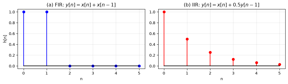
Compute the first 6 samples (\(n = 0\) to \(5\)) of the impulse response for each system. The input is \(x[n] = \delta[n]\) and all initial conditions are zero.
\(y[n] = x[n] + x[n-1]\) (2-tap FIR)
\(y[n] = x[n] + 0.5\,y[n-1]\) (first-order IIR)
Solution
FIR: \(h = [1, 1, 0, 0, 0, 0]\). The impulse response equals the coefficients.
Sign convention note: The lfilter call uses a = [1, -0.5] because lfilter solves \(\sum a_j\,y[n-j] = \sum b_i\,x[n-i]\), i.e. \(y[n] - 0.5\,y[n-1] = x[n]\). The minus sign in the a vector corresponds to the plus sign in our difference equation \(y[n] = x[n] + 0.5\,y[n-1]\).
Exercise 4: Linearity test
A system is defined by \(y[n] = x[n]^2\). Is it linear?
Test by checking the superposition principle: apply inputs \(x_1[n] = \delta[n]\) and \(x_2[n] = 2\,\delta[n-1]\) separately and combined. Does \(T\{x_1 + x_2\} = T\{x_1\} + T\{x_2\}\)?
This filter is a first-order differencer (\(h = [1, -1]\)). It computes the difference between successive samples, a discrete approximation to the derivative.
Exercise 6: DC gain
The DC gain of a filter is its response to a constant (DC) input. If \(x[n] = 1\) for all \(n\), then after transients die out, the output settles to a constant \(y[n] = G\), where \(G\) is the DC gain.
For an FIR filter, show that the DC gain equals the sum of the coefficients: \(G = \sum_i b_i\).
Then compute the DC gain for:
\(h = [1/3, 1/3, 1/3]\) (3-point MA)
\(h = [1, -1]\) (differencer)
\(h = [0.25, 0.5, 0.25]\) (weighted average)
Solution
If \(x[n] = 1\) for all \(n\), then: \[y[n] = \sum_{i=0}^P b_i \cdot x[n-i] = \sum_{i=0}^P b_i \cdot 1 = \sum_{i=0}^P b_i\]
\(G = 1/3 + 1/3 + 1/3 = 1\): the MA preserves DC level (good for smoothing).
\(G = 1 + (-1) = 0\): the differencer removes DC entirely (it’s a high-pass filter).
import numpy as npfilters = {"3-pt MA": [1/3, 1/3, 1/3],"Differencer": [1, -1],"Weighted avg": [0.25, 0.5, 0.25],}for name, h in filters.items():print(f"{name:15s} DC gain = {sum(h):.4f}")
3-pt MA          DC gain = 1.0000
Differencer      DC gain = 0.0000
Weighted avg     DC gain = 1.0000
DC gain is a quick sanity check: a smoothing filter should have DC gain = 1 (it preserves the mean), while a differencing filter should have DC gain = 0 (it removes the mean).
Exercise 7: Cascaded filters
Two FIR filters are applied in sequence (cascaded):
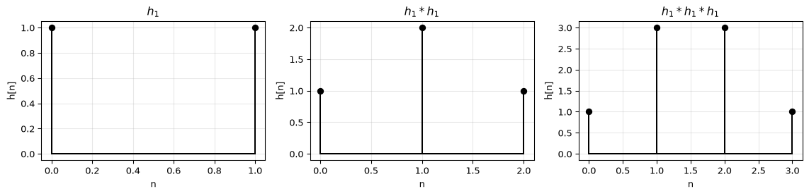
\[h_1 = [1, 1], \quad h_2 = [1, 1]\]
What is the impulse response of the cascaded system \(h = h_1 * h_2\)?
What familiar filter does the cascade implement?
Now cascade three copies: \(h_1 * h_1 * h_1\). What does the impulse response look like?
Solution
import numpy as npimport matplotlib.pyplot as plth1 = np.array([1, 1])h2 = np.array([1, 1])h_cascade = np.convolve(h1, h2)print(f"h1 * h2 = {h_cascade}")
h1 * h2 = [1 2 1]
The result is \([1, 2, 1]\): a triangular window. This is a weighted moving average.
This is equivalent to the single filter \(y[n] = x[n] + 2\,x[n-1] + x[n-2]\). Normalised by the DC gain (4), it gives \([0.25, 0.5, 0.25]\), the weighted average from Exercise 6c.
\([1, 3, 3, 1]\): the binomial coefficients. Repeated convolution of a rectangular pulse approaches a Gaussian shape (central limit theorem). This is the basis of Gaussian smoothing.
Exercise 8: IIR filter step-by-step
A first-order IIR filter has the difference equation:
\[y[n] = x[n] - 0.5\,y[n-1]\]
Given input \(x = [1, 0, 0, 0, 0, 0, 0, 0]\) (an impulse), compute \(y[n]\) for \(n = 0\) to \(7\) by hand, then verify with lfilter.
Solution
n
x[n]
y[n-1]
y[n] = x[n] − 0.5·y[n-1]
0
1
0
1.0
1
0
1.0
−0.5
2
0
−0.5
0.25
3
0
0.25
−0.125
4
0
−0.125
0.0625
5
0
0.0625
−0.03125
6
0
−0.03125
0.015625
7
0
0.015625
−0.0078125
The pattern is \(h[n] = (-0.5)^n\): alternating, decaying.
The general rule for geometric sequences: \(h[n] = a^n \cdot u[n]\) is stable if and only if \(|a| < 1\).
Exercise 10: Implement a filter from scratch
Implement a function apply_filter(b, a, x) that applies a difference equation to an input signal, without using lfilter or convolve. Your function should:
Accept feedforward coefficients b, feedback coefficients a (where a[0] = 1), and input x
Return the output y of the same length as x
Assume zero initial conditions
Test it on the MA filter (\(b = [1/3, 1/3, 1/3]\), \(a = [1]\)) and the first-order IIR (\(b = [1]\), \(a = [1, -0.8]\)).
Solution
import numpy as npfrom scipy.signal import lfilterdef apply_filter(b, a, x):"""Apply a difference equation y[n] = sum(b_i * x[n-i]) - sum(a_j * y[n-j]).""" b = np.asarray(b, dtype=float) a = np.asarray(a, dtype=float) x = np.asarray(x, dtype=float) N =len(x) P =len(b) -1# feedforward order Q =len(a) -1# feedback order y = np.zeros(N)for n inrange(N):# Feedforward: sum of b_i * x[n-i]for i inrange(len(b)):if n - i >=0: y[n] += b[i] * x[n - i]# Feedback: subtract sum of a_j * y[n-j]for j inrange(1, len(a)):if n - j >=0: y[n] -= a[j] * y[n - j]# Normalise by a[0] y[n] /= a[0]return y# Test: MA filternp.random.seed(0)x = np.random.randn(20)b_ma = [1/3, 1/3, 1/3]y_ours = apply_filter(b_ma, [1], x)y_ref = lfilter(b_ma, [1], x)print(f"MA filter match: {np.allclose(y_ours, y_ref)}")# Test: IIR filterb_iir = [1]a_iir = [1, -0.8]y_ours = apply_filter(b_iir, a_iir, x)y_ref = lfilter(b_iir, a_iir, x)print(f"IIR filter match: {np.allclose(y_ours, y_ref)}")
MA filter match: True
IIR filter match: True
This is the core of any DSP system: the difference equation loop. On a microcontroller, this runs at interrupt rate: one iteration per sample.
Exercise 11: Exponential moving average tuning
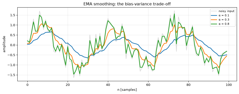
The exponential moving average (EMA) is a first-order IIR filter:
\[y[n] = \alpha\, x[n] + (1 - \alpha)\, y[n-1]\]
where \(0 < \alpha \leq 1\) controls the smoothing. Smaller \(\alpha\) = more smoothing.
Show that the DC gain is 1 for any \(\alpha\).
Show that the impulse response is \(h[n] = \alpha\,(1-\alpha)^n\) for \(n \geq 0\).
Write Python code that applies the EMA with three different \(\alpha\) values (0.1, 0.3, 0.8) to a noisy sinusoid. Plot the results and discuss the trade-off.
Solution
For DC input \(x[n] = 1\): \(y = \alpha \cdot 1 + (1-\alpha) \cdot y\), so \(y - (1-\alpha)y = \alpha\), giving \(\alpha y = \alpha\), hence \(y = 1\). DC gain is 1 for any \(\alpha\).
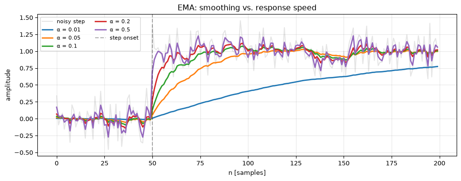
import numpy as npimport matplotlib.pyplot as pltfrom scipy.signal import lfilternp.random.seed(42)n = np.arange(100)x = np.sin(2* np.pi *0.03* n) +0.5* np.random.randn(len(n))fig, ax = plt.subplots(figsize=(10, 4))ax.plot(n, x, 'C7-', alpha=0.3, label='noisy input')for alpha in [0.1, 0.3, 0.8]: y = lfilter([alpha], [1, -(1- alpha)], x) ax.plot(n, y, linewidth=2, label=f'α = {alpha}')ax.set_xlabel('n [samples]')ax.set_ylabel('amplitude')ax.legend(fontsize=8)ax.grid(True, alpha=0.3)ax.set_title('EMA smoothing: the bias-variance trade-off')plt.tight_layout()plt.show()
\(\alpha = 0.1\): Heavy smoothing, low noise, but lags the true signal significantly (high bias, low variance).
\(\alpha = 0.8\): Light smoothing, fast tracking, but noisy output (low bias, high variance).
\(\alpha = 0.3\): A reasonable compromise for many applications.
This bias-variance trade-off is fundamental to all filter design.
Exercise 12: Debug this: unstable filter
Challenge. Consider the following IIR filter:
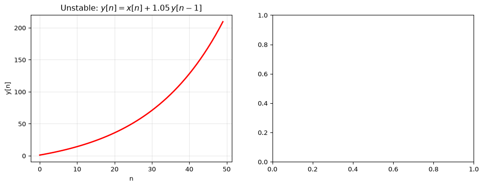
\[y[n] = x[n] + 1.05\,y[n-1]\]
Implement this filter and apply it to a unit step input of length 50. Plot the output.
Explain why the output explodes.
Fix the filter by adjusting the feedback coefficient. Show the corrected output.
Solution
The output grows without bound:
import numpy as npimport matplotlib.pyplot as pltfrom scipy.signal import lfilterx = np.ones(50) # unit step# Unstable filter: pole at z = 1.05y_unstable = lfilter([1], [1, -1.05], x)fig, axes = plt.subplots(1, 2, figsize=(12, 4))axes[0].plot(y_unstable, 'r-', linewidth=2)axes[0].set_title('Unstable: $y[n] = x[n] + 1.05\\,y[n-1]$')axes[0].set_xlabel('n')axes[0].set_ylabel('y[n]')axes[0].grid(True, alpha=0.3)
The feedback coefficient 1.05 means the pole of the system is at \(z = 1.05\), which lies outside the unit circle. For BIBO stability, all poles must be strictly inside the unit circle (\(|z| < 1\)). Because \(|1.05| > 1\), the impulse response \(h[n] = 1.05^n\) grows exponentially.
Changing the coefficient to 0.95 places the pole inside the unit circle:
# Stable filter: pole at z = 0.95y_stable = lfilter([1], [1, -0.95], x)axes[1].plot(x, 'C7--', alpha=0.5, label='input (step)')axes[1].plot(y_stable, 'b-', linewidth=2, label='output')axes[1].set_title('Stable: $y[n] = x[n] + 0.95\\,y[n-1]$')axes[1].set_xlabel('n')axes[1].set_ylabel('y[n]')axes[1].legend()axes[1].grid(True, alpha=0.3)plt.tight_layout()plt.show()
<Figure size 672x480 with 0 Axes>
The stable filter acts as a leaky integrator, and the output rises toward a steady-state value of \(1/(1-0.95) = 20\).
Exercise 13: Identify FIR vs IIR from code
Intermediate. Three filters are defined by their (b, a) coefficient pairs and applied using scipy.signal.lfilter:
If IIR, compute the poles and determine if the filter is stable.
What is the DC gain?
Solution
import numpy as npfilters = {"A": {"b": [0.2, 0.6, 0.2], "a": [1]},"B": {"b": [1, -1], "a": [1, -0.9]},"C": {"b": [0.1, 0.2, 0.3, 0.2, 0.1], "a": [1]},}for name, f in filters.items(): b, a = np.array(f["b"]), np.array(f["a"]) is_fir =len(a) ==1and a[0] ==1 dc_gain =sum(b) /sum(a) # DC gain = H(z=1) = sum(b) / sum(a), valid when a[0] = 1 (lfilter convention)print(f"Filter {name}:")print(f" Type: {'FIR'if is_fir else'IIR'}")ifnot is_fir: poles = np.roots(a) stable =all(np.abs(poles) <1)print(f" Poles: {poles}")print(f" Stable: {stable}")print(f" DC gain: {dc_gain:.4f}")print()
Filter A:
  Type: FIR
  DC gain: 1.0000

Filter B:
  Type: IIR
  Poles: [0.9]
  Stable: True
  DC gain: 0.0000

Filter C:
  Type: FIR
  DC gain: 0.9000
Filter A: FIR (a=[1]). It is a 3-tap weighted average with DC gain = 1.0.
Filter B: IIR (a=[1, -0.9]). It has one pole at \(z = 0.9\), which is inside the unit circle → stable. DC gain = \((1-1)/(1-0.9) = 0\): this is a high-pass filter.
Filter C: FIR (a=[1]). A symmetric 5-tap filter with DC gain = 0.9. Note: a DC gain below 1.0 means this filter attenuates even constant signals by 10%; to make it a unity-gain lowpass, normalise the coefficients to sum to 1.
Rule of thumb: If a = [1], the filter is FIR (no feedback). Any other a vector means feedback is present → IIR.
Exercise 14: System identification from impulse response
Intermediate. You have recorded the impulse response of an unknown system:
\[h = [1,\; 0.5,\; -0.3,\; 0.1]\]
Is this system FIR or IIR?
What are the filter coefficients?
Write the transfer function \(H(z)\).
Compute and plot the step response.
Solution
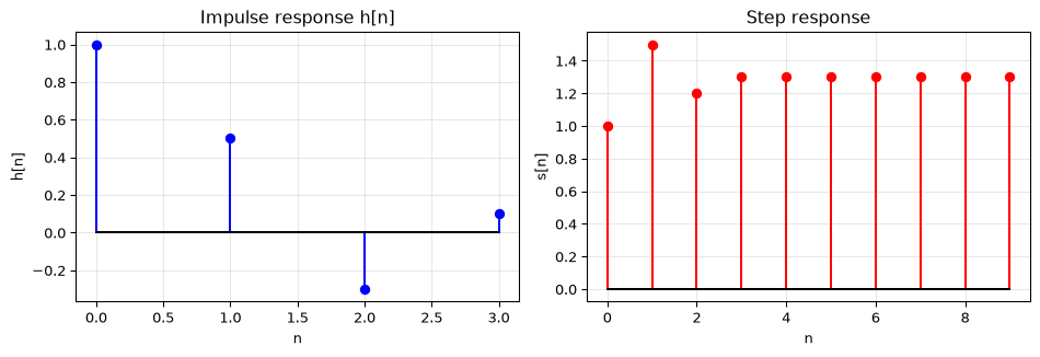
The impulse response is finite (4 samples, then zero) → this is an FIR filter.
For an FIR filter, the impulse response is the set of feedforward coefficients: \(b = [1, 0.5, -0.3, 0.1]\), \(a = [1]\).
The transfer function is: \[H(z) = 1 + 0.5\,z^{-1} - 0.3\,z^{-2} + 0.1\,z^{-3}\]
The step response is the cumulative sum of the impulse response:
import numpy as npimport matplotlib.pyplot as pltfrom scipy.signal import lfilterh = np.array([1, 0.5, -0.3, 0.1])# Step response = filter applied to unit stepN =10step_input = np.ones(N)step_response = lfilter(h, [1], step_input)# Equivalently: cumulative sum of the impulse response (zero-padded)h_padded = np.zeros(N)h_padded[:len(h)] = hstep_cumsum = np.cumsum(h_padded)fig, axes = plt.subplots(1, 2, figsize=(10, 3.5))axes[0].stem(np.arange(len(h)), h, linefmt='b-', markerfmt='bo', basefmt='k-')axes[0].set_title('Impulse response h[n]')axes[0].set_xlabel('n')axes[0].set_ylabel('h[n]')axes[0].grid(True, alpha=0.3)axes[1].stem(np.arange(N), step_response, linefmt='r-', markerfmt='ro', basefmt='k-')axes[1].set_title('Step response')axes[1].set_xlabel('n')axes[1].set_ylabel('s[n]')axes[1].grid(True, alpha=0.3)plt.tight_layout()plt.show()print(f"Step response: {step_response}")print(f"Cumsum check: {step_cumsum}")print(f"DC gain (final value): {sum(h):.1f}")
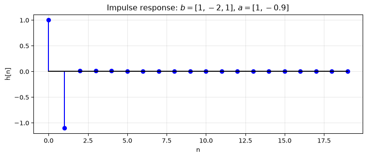
The feedforward coefficients \([1, -2, 1]\) implement a second-order difference (discrete second derivative): this is a highpass characteristic. The feedback coefficient \(0.9\) adds resonance (the pole at \(z = 0.9\) is close to the unit circle, giving a long decay). This is an IIR highpass filter with a slowly decaying impulse response. The DC gain is \((1-2+1)/(1-0.9) = 0\), confirming the highpass behaviour.
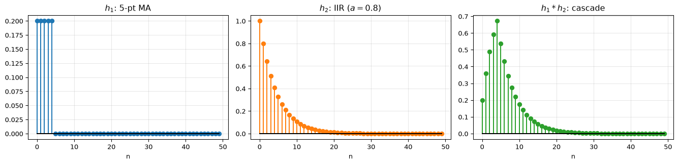
Exercise 18: Cascaded systems analysis
Challenge. Two filters are cascaded (applied in series):
# (b) Sequential vs cascadenp.random.seed(0)x = np.random.randn(200)# Sequential: MA first, then IIRy_seq_12 = lfilter(b2, a2, lfilter(b1, a1, x))# Using convolved impulse responsey_cascade = lfilter(h_conv, [1], x)[:len(x)]# Approximate match: h_conv is truncated to N=50 samplesprint(f"Sequential == cascade: {np.allclose(y_seq_12, y_cascade, atol=1e-3)}")# (c) Reverse order: IIR first, then MAy_seq_21 = lfilter(b1, a1, lfilter(b2, a2, x))print(f"Order 1→2 == Order 2→1: {np.allclose(y_seq_12, y_seq_21)}")
Sequential == cascade: True
Order 1→2 == Order 2→1: True
Yes, the cascade is commutative. For LTI systems, cascading is equivalent to convolving the impulse responses, and convolution is commutative (\(h_1 * h_2 = h_2 * h_1\)). The order does not matter for the final result, though in practice, putting the MA filter first can reduce the dynamic range seen by the IIR stage.
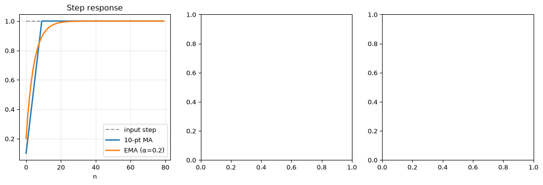
Exercise 19: Moving average vs exponential moving average
Challenge. Compare a 10-point moving average (MA) filter with an exponential moving average (EMA) with \(\alpha = 0.2\) (which gives roughly equivalent smoothing).
Process a noisy step signal and compare:
Step response delay
Noise reduction (SNR improvement)
Frequency response (use scipy.signal.freqz)
Which filter is better for real-time applications and why?
Step response: The MA has a fixed delay of \((L-1)/2 = 4.5\) samples (a non-integer delay; for even-length FIR filters, perfect alignment requires fractional-sample interpolation; odd-length filters avoid this issue). The EMA responds immediately (no group delay at DC), but approaches the final value exponentially.
Noise reduction: Both provide similar SNR improvement (~10 dB). The MA provides slightly better noise rejection because its frequency response has nulls (zeros) at specific frequencies.
Frequency response: The MA has sharp nulls at multiples of \(f_s/10\). The EMA has a smooth, monotonically decreasing response.
For real-time applications, the EMA is often preferred because: (1) it requires only one multiply-add per sample (vs. \(L\) for the MA), (2) it needs only one state variable (vs. an \(L\)-sample buffer), and (3) its response time is tunable with a single parameter.
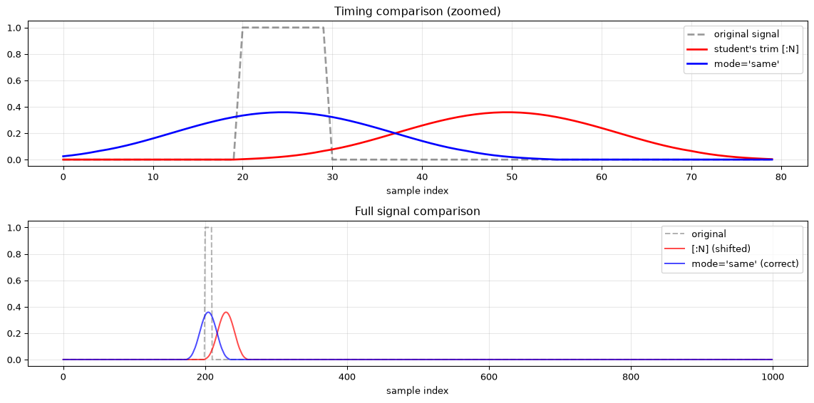
fig, axes = plt.subplots(2, 1, figsize=(12, 6))# Zoom into the pulse regionregion =slice(180, 260)axes[0].plot(x[region], 'k--', alpha=0.4, linewidth=2, label='original signal')axes[0].plot(y_wrong[region], 'r-', linewidth=2, label="student's trim [:N]")axes[0].plot(y_same[region], 'b-', linewidth=2, label="mode='same'")axes[0].set_title('Timing comparison (zoomed)')axes[0].set_xlabel('sample index')axes[0].legend()axes[0].grid(True, alpha=0.3)# Show the full signalaxes[1].plot(x, 'k--', alpha=0.3, label='original')axes[1].plot(y_wrong, 'r-', alpha=0.7, label="[:N] (shifted)")axes[1].plot(y_same, 'b-', alpha=0.7, label="mode='same' (correct)")axes[1].set_title('Full signal comparison')axes[1].set_xlabel('sample index')axes[1].legend()axes[1].grid(True, alpha=0.3)plt.tight_layout()plt.show()delay = (L -1) //2print(f"\nThe student's trim introduces a {delay}-sample delay.")print(f"The pulse peak appears at index {np.argmax(y_wrong)} instead of ~{np.argmax(y_same)}.")
The student's trim introduces a 25-sample delay.
The pulse peak appears at index 229 instead of ~204.
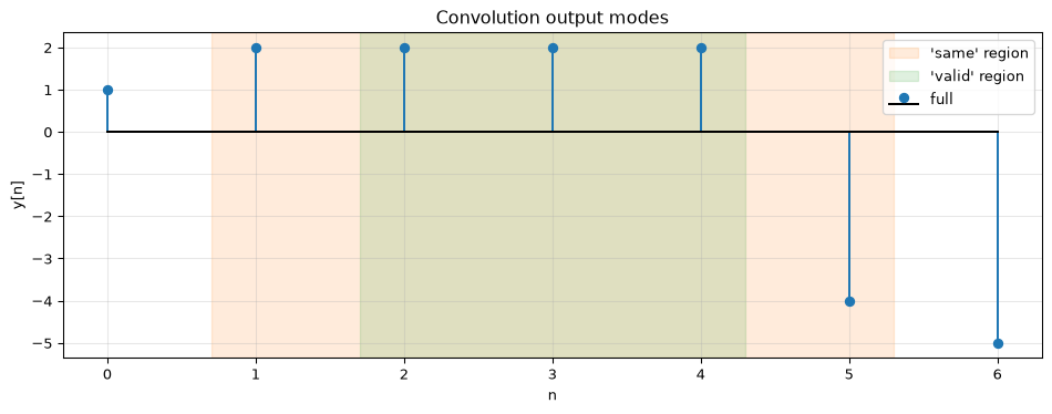
What went wrong:np.convolve in full mode prepends \((L-1)/2 = 25\) samples of transient before the first “real” output. By taking y[:N], the student keeps these transients and chops off the last 25 valid samples. The entire output is shifted by 25 samples to the right.
Correct approaches:
mode='same' automatically centres the output, discarding equal amounts from both ends.
Manual alignment: skip the first (L-1)//2 samples of the full output: y_full[25:1025].
This is a common bug in practice: always be explicit about which convolution mode you need.
Source Code
---title: "Exercises: Discrete-Time Systems"subtitle: "Practice problems for Chapter 2"---These exercises accompany [Chapter 2: Discrete-Time Systems](../basics/02-discrete-time.qmd).::: {.callout-note title="Key formulas for this chapter"}| Formula | Description ||---------|-------------|| $y[n] = \sum_{i=0}^{P} b_i\,x[n-i] - \sum_{j=1}^{Q} a_j\,y[n-j]$ | General difference equation || Output length: $L_x + L_h - 1$ | FIR convolution output length || BIBO stability: $\sum_{n=0}^{\infty} \lvert h[n]\rvert < \infty$ | All poles inside unit circle || DC gain: $H(1) = \sum b_i \,/\, \sum a_j$ | Evaluate transfer function at $z=1$ || EMA: $y[n] = \alpha\,x[n] + (1-\alpha)\,y[n-1]$ | Exponential moving average || EMA impulse response: $h[n] = \alpha(1-\alpha)^n$ | Geometric decay |:::## Basic::: {.callout-tip collapse="true" title="Exercise 1: Filter coefficients from difference equations"}For each difference equation, identify the feedforward coefficients $b_i$, the feedback coefficients $a_j$, and classify the filter as FIR or IIR.a) $y[n] = 2\,x[n] - x[n-1]$b) $y[n] = x[n-2]$c) $y[n] = x[n] - 2\,x[n-1] + 2\,x[n-2] + x[n-3]$d) $y[n] = 0.5\,x[n] + 0.8\,y[n-1]$::: {.callout-note collapse="true" title="Solution"}a) $b = [2, -1]$, no feedback → **FIR**, order 1b) $b = [0, 0, 1]$, no feedback → **FIR**, order 2 (a pure delay of 2 samples)c) $b = [1, -2, 2, 1]$, no feedback → **FIR**, order 3d) $b = [0.5]$, $a = [1, -0.8]$ → **IIR**, order 1 (first-order recursive filter with feedback)::::::::: {.callout-tip collapse="true" title="Exercise 2: MA filter step-by-step"}A 2nd-order MA filter has the difference equation:$$y[n] = \tfrac{1}{3}\bigl(x[n] + x[n-1] + x[n-2]\bigr)$$Given the input sequence $x = [2, -1, 3, 0, -2]$, compute the output $y[n]$ for $n = 0, 1, 2, 3, 4$. Assume $x[n] = 0$ for $n < 0$.::: {.callout-note collapse="true" title="Solution"}```{python}import numpy as npx = np.array([2, -1, 3, 0, -2])print(f"{'n':>3s}{'x[n]':>6s}{'x[n-1]':>7s}{'x[n-2]':>7s}{'y[n]':>8s}")print("-"*38)for i inrange(len(x)): xn = x[i] xn1 = x[i -1] if i >=1else0 xn2 = x[i -2] if i >=2else0 yn = (xn + xn1 + xn2) /3print(f"{i:3d}{xn:6.1f}{xn1:7.1f}{xn2:7.1f}{yn:8.4f}")```::::::::: {.callout-tip collapse="true" title="Exercise 3: Impulse response by hand"}Compute the first 6 samples ($n = 0$ to $5$) of the impulse response for each system. The input is $x[n] = \delta[n]$ and all initial conditions are zero.a) $y[n] = x[n] + x[n-1]$ (2-tap FIR)b) $y[n] = x[n] + 0.5\,y[n-1]$ (first-order IIR)::: {.callout-note collapse="true" title="Solution"}a) FIR: $h = [1, 1, 0, 0, 0, 0]$. The impulse response equals the coefficients.b) IIR: $h[0] = 1$, $h[1] = 0.5$, $h[2] = 0.25$, $h[3] = 0.125$, $h[4] = 0.0625$, $h[5] = 0.03125$. In general $h[n] = 0.5^n$.```{python}import numpy as npimport matplotlib.pyplot as pltfrom scipy.signal import lfilterdelta = np.zeros(6)delta[0] =1h_fir = lfilter([1, 1], [1], delta)h_iir = lfilter([1], [1, -0.5], delta)fig, axes = plt.subplots(1, 2, figsize=(10, 3))axes[0].stem(np.arange(6), h_fir, linefmt='b-', markerfmt='bo', basefmt='k-')axes[0].set_title('(a) FIR: $y[n] = x[n] + x[n-1]$')axes[0].set_xlabel('n')axes[0].set_ylabel('h[n]')axes[0].grid(True, alpha=0.3)axes[1].stem(np.arange(6), h_iir, linefmt='r-', markerfmt='ro', basefmt='k-')axes[1].set_title('(b) IIR: $y[n] = x[n] + 0.5 y[n-1]$')axes[1].set_xlabel('n')axes[1].grid(True, alpha=0.3)plt.tight_layout()plt.show()```**Sign convention note:** The `lfilter` call uses `a = [1, -0.5]` because `lfilter` solves $\sum a_j\,y[n-j] = \sum b_i\,x[n-i]$, i.e. $y[n] - 0.5\,y[n-1] = x[n]$. The minus sign in the `a` vector corresponds to the plus sign in our difference equation $y[n] = x[n] + 0.5\,y[n-1]$.::::::::: {.callout-tip collapse="true" title="Exercise 4: Linearity test"}A system is defined by $y[n] = x[n]^2$. Is it linear?Test by checking the superposition principle: apply inputs $x_1[n] = \delta[n]$ and $x_2[n] = 2\,\delta[n-1]$ separately and combined. Does $T\{x_1 + x_2\} = T\{x_1\} + T\{x_2\}$?::: {.callout-note collapse="true" title="Solution"}```{python}import numpy as npx1 = np.array([1, 0, 0, 0]) # delta[n]x2 = np.array([0, 2, 0, 0]) # 2*delta[n-1]y1 = x1 **2# [1, 0, 0, 0]y2 = x2 **2# [0, 4, 0, 0]y_sum = y1 + y2 # [1, 4, 0, 0]y_combined = (x1 + x2) **2# [1, 4, 0, 0] ... waitprint("y1 = ", y1)print("y2 = ", y2)print("y1 + y2 = ", y_sum)print("T{x1 + x2} = ", y_combined)print("Equal? ", np.allclose(y_sum, y_combined))```They happen to be equal for this specific input. That's a coincidence (the non-zero values don't overlap). Try $x_1 = [1, 0]$ and $x_2 = [1, 0]$:```{python}x1 = np.array([1, 0])x2 = np.array([1, 0])y1 = x1 **2# [1, 0]y2 = x2 **2# [1, 0]y_sum = y1 + y2 # [2, 0]y_combined = (x1 + x2) **2# [4, 0]print("y1 + y2 = ", y_sum)print("T{x1 + x2} = ", y_combined)print("Equal? ", np.allclose(y_sum, y_combined))```**Not linear.** $(x_1 + x_2)^2 = x_1^2 + 2x_1 x_2 + x_2^2 \neq x_1^2 + x_2^2$. The cross-term $2 x_1 x_2$ violates superposition. Squaring is a nonlinear operation.::::::## Intermediate::: {.callout-tip collapse="true" title="Exercise 5: Convolution by hand and by code"}Compute the convolution $y[n] = x[n] * h[n]$ for:$$x = [1, 2, 3], \quad h = [1, -1]$$a) Do it by hand (write out each output sample).b) Verify using `np.convolve`.c) What is the length of $y$?::: {.callout-note collapse="true" title="Solution"}a) Using the convolution sum $y[n] = \sum_{k} h[k] \cdot x[n-k]$:- $y[0] = h[0]\,x[0] + h[1]\,x[-1] = 1 \cdot 1 + (-1) \cdot 0 = 1$- $y[1] = h[0]\,x[1] + h[1]\,x[0] = 1 \cdot 2 + (-1) \cdot 1 = 1$- $y[2] = h[0]\,x[2] + h[1]\,x[1] = 1 \cdot 3 + (-1) \cdot 2 = 1$- $y[3] = h[0]\,x[3] + h[1]\,x[2] = 1 \cdot 0 + (-1) \cdot 3 = -3$So $y = [1, 1, 1, -3]$.b)```{python}import numpy as npx = np.array([1, 2, 3])h = np.array([1, -1])y = np.convolve(x, h)print(f"y = {y}")print(f"Length: {len(x)} + {len(h)} - 1 = {len(y)}")```c) $\text{len}(y) = 3 + 2 - 1 = 4$.This filter is a **first-order differencer** ($h = [1, -1]$). It computes the difference between successive samples, a discrete approximation to the derivative.::::::::: {.callout-tip collapse="true" title="Exercise 6: DC gain"}The **DC gain** of a filter is its response to a constant (DC) input. If $x[n] = 1$ for all $n$, then after transients die out, the output settles to a constant $y[n] = G$, where $G$ is the DC gain.For an FIR filter, show that the DC gain equals the sum of the coefficients: $G = \sum_i b_i$.Then compute the DC gain for:a) $h = [1/3, 1/3, 1/3]$ (3-point MA)b) $h = [1, -1]$ (differencer)c) $h = [0.25, 0.5, 0.25]$ (weighted average)::: {.callout-note collapse="true" title="Solution"}If $x[n] = 1$ for all $n$, then:$$y[n] = \sum_{i=0}^P b_i \cdot x[n-i] = \sum_{i=0}^P b_i \cdot 1 = \sum_{i=0}^P b_i$$a) $G = 1/3 + 1/3 + 1/3 = 1$: the MA preserves DC level (good for smoothing).b) $G = 1 + (-1) = 0$: the differencer removes DC entirely (it's a high-pass filter).c) $G = 0.25 + 0.5 + 0.25 = 1$: DC-preserving weighted average.```{python}import numpy as npfilters = {"3-pt MA": [1/3, 1/3, 1/3],"Differencer": [1, -1],"Weighted avg": [0.25, 0.5, 0.25],}for name, h in filters.items():print(f"{name:15s} DC gain = {sum(h):.4f}")```DC gain is a quick sanity check: a smoothing filter should have DC gain = 1 (it preserves the mean), while a differencing filter should have DC gain = 0 (it removes the mean).::::::::: {.callout-tip collapse="true" title="Exercise 7: Cascaded filters"}Two FIR filters are applied in sequence (cascaded):$$h_1 = [1, 1], \quad h_2 = [1, 1]$$a) What is the impulse response of the cascaded system $h = h_1 * h_2$?b) What familiar filter does the cascade implement?c) Now cascade three copies: $h_1 * h_1 * h_1$. What does the impulse response look like?::: {.callout-note collapse="true" title="Solution"}a)```{python}import numpy as npimport matplotlib.pyplot as plth1 = np.array([1, 1])h2 = np.array([1, 1])h_cascade = np.convolve(h1, h2)print(f"h1 * h2 = {h_cascade}")```The result is $[1, 2, 1]$: a triangular window. This is a weighted moving average.b) This is equivalent to the single filter $y[n] = x[n] + 2\,x[n-1] + x[n-2]$. Normalised by the DC gain (4), it gives $[0.25, 0.5, 0.25]$, the weighted average from Exercise 6c.c) Cascading three times:```{python}h_triple = np.convolve(np.convolve(h1, h1), h1)fig, axes = plt.subplots(1, 3, figsize=(12, 3))for ax, h, title inzip(axes, [h1, h_cascade, h_triple], ['$h_1$', '$h_1 * h_1$', '$h_1 * h_1 * h_1$']): ax.stem(np.arange(len(h)), h, linefmt='k-', markerfmt='ko', basefmt='k-') ax.set_title(title) ax.set_xlabel('n') ax.set_ylabel('h[n]') ax.grid(True, alpha=0.3)plt.tight_layout()plt.show()print(f"h1 * h1 * h1 = {h_triple}")```$[1, 3, 3, 1]$: the binomial coefficients. Repeated convolution of a rectangular pulse approaches a Gaussian shape (central limit theorem). This is the basis of Gaussian smoothing.::::::::: {.callout-tip collapse="true" title="Exercise 8: IIR filter step-by-step"}A first-order IIR filter has the difference equation:$$y[n] = x[n] - 0.5\,y[n-1]$$Given input $x = [1, 0, 0, 0, 0, 0, 0, 0]$ (an impulse), compute $y[n]$ for $n = 0$ to $7$ by hand, then verify with `lfilter`.::: {.callout-note collapse="true" title="Solution"}| n | x[n] | y[n-1] | y[n] = x[n] − 0.5·y[n-1] ||---|------|--------|--------------------------|| 0 | 1 | 0 | 1.0 || 1 | 0 | 1.0 | −0.5 || 2 | 0 | −0.5 | 0.25 || 3 | 0 | 0.25 | −0.125 || 4 | 0 | −0.125 | 0.0625 || 5 | 0 | 0.0625 | −0.03125 || 6 | 0 | −0.03125 | 0.015625 || 7 | 0 | 0.015625 | −0.0078125 |The pattern is $h[n] = (-0.5)^n$: alternating, decaying.```{python}import numpy as npfrom scipy.signal import lfilterx = np.zeros(8)x[0] =1y = lfilter([1], [1, 0.5], x) # b=[1], a=[1, 0.5] → y[n] + 0.5*y[n-1] = x[n]print(f"{'n':>3s}{'h[n] (lfilter)':>14s}{'(-0.5)^n':>10s}")print("-"*32)for n inrange(8):print(f"{n:3d}{y[n]:14.6f}{(-0.5)**n:10.6f}")```Note the sign convention: `lfilter([1], [1, 0.5], x)` corresponds to $y[n] + 0.5\,y[n-1] = x[n]$, which is the same as $y[n] = x[n] - 0.5\,y[n-1]$.::::::## Challenge::: {.callout-tip collapse="true" title="Exercise 9: BIBO stability analysis"}Determine whether each system is BIBO stable by checking if $\sum |h[n]| < \infty$.a) $h[n] = 0.9^n \cdot u[n]$ (where $u[n]$ is the unit step)b) $h[n] = u[n]$ (integrator / accumulator)c) $h[n] = (-1)^n \cdot 0.5^n \cdot u[n]$For each, compute the sum analytically and verify numerically.::: {.callout-note collapse="true" title="Solution"}a) $\sum_{n=0}^{\infty} |0.9^n| = \sum_{n=0}^{\infty} 0.9^n = \frac{1}{1 - 0.9} = 10 < \infty$ → **Stable**.b) $\sum_{n=0}^{\infty} |1| = \infty$ → **Unstable**. The accumulator (running sum) grows without bound for any non-zero DC input.c) $\sum_{n=0}^{\infty} |(-0.5)^n| = \sum_{n=0}^{\infty} 0.5^n = \frac{1}{1 - 0.5} = 2 < \infty$ → **Stable**.```{python}import numpy as npN =1000# approximate infinity# (a)h_a =0.9** np.arange(N)print(f"(a) sum|h| = {np.sum(np.abs(h_a)):.4f} (analytical: {1/(1-0.9):.1f})")# (b)h_b = np.ones(N)print(f"(b) sum|h| = {np.sum(np.abs(h_b)):.0f} (diverges)")# (c)h_c = (-0.5) ** np.arange(N)print(f"(c) sum|h| = {np.sum(np.abs(h_c)):.4f} (analytical: {1/(1-0.5):.1f})")```The general rule for geometric sequences: $h[n] = a^n \cdot u[n]$ is stable if and only if $|a| < 1$.::::::::: {.callout-tip collapse="true" title="Exercise 10: Implement a filter from scratch"}Implement a function `apply_filter(b, a, x)` that applies a difference equation to an input signal, without using `lfilter` or `convolve`. Your function should:1. Accept feedforward coefficients `b`, feedback coefficients `a` (where `a[0]` = 1), and input `x`2. Return the output `y` of the same length as `x`3. Assume zero initial conditionsTest it on the MA filter ($b = [1/3, 1/3, 1/3]$, $a = [1]$) and the first-order IIR ($b = [1]$, $a = [1, -0.8]$).::: {.callout-note collapse="true" title="Solution"}```{python}import numpy as npfrom scipy.signal import lfilterdef apply_filter(b, a, x):"""Apply a difference equation y[n] = sum(b_i * x[n-i]) - sum(a_j * y[n-j]).""" b = np.asarray(b, dtype=float) a = np.asarray(a, dtype=float) x = np.asarray(x, dtype=float) N =len(x) P =len(b) -1# feedforward order Q =len(a) -1# feedback order y = np.zeros(N)for n inrange(N):# Feedforward: sum of b_i * x[n-i]for i inrange(len(b)):if n - i >=0: y[n] += b[i] * x[n - i]# Feedback: subtract sum of a_j * y[n-j]for j inrange(1, len(a)):if n - j >=0: y[n] -= a[j] * y[n - j]# Normalise by a[0] y[n] /= a[0]return y# Test: MA filternp.random.seed(0)x = np.random.randn(20)b_ma = [1/3, 1/3, 1/3]y_ours = apply_filter(b_ma, [1], x)y_ref = lfilter(b_ma, [1], x)print(f"MA filter match: {np.allclose(y_ours, y_ref)}")# Test: IIR filterb_iir = [1]a_iir = [1, -0.8]y_ours = apply_filter(b_iir, a_iir, x)y_ref = lfilter(b_iir, a_iir, x)print(f"IIR filter match: {np.allclose(y_ours, y_ref)}")```This is the core of any DSP system: the difference equation loop. On a microcontroller, this runs at interrupt rate: one iteration per sample.::::::::: {.callout-tip collapse="true" title="Exercise 11: Exponential moving average tuning"}The **exponential moving average** (EMA) is a first-order IIR filter:$$y[n] = \alpha\, x[n] + (1 - \alpha)\, y[n-1]$$where $0 < \alpha \leq 1$ controls the smoothing. Smaller $\alpha$ = more smoothing.a) Show that the DC gain is 1 for any $\alpha$.b) Show that the impulse response is $h[n] = \alpha\,(1-\alpha)^n$ for $n \geq 0$.c) Write Python code that applies the EMA with three different $\alpha$ values (0.1, 0.3, 0.8) to a noisy sinusoid. Plot the results and discuss the trade-off.::: {.callout-note collapse="true" title="Solution"}a) For DC input $x[n] = 1$: $y = \alpha \cdot 1 + (1-\alpha) \cdot y$, so $y - (1-\alpha)y = \alpha$, giving $\alpha y = \alpha$, hence $y = 1$. DC gain is 1 for any $\alpha$.b) For impulse input: $h[0] = \alpha$, $h[1] = (1-\alpha)\alpha$, $h[n] = (1-\alpha)^n \alpha$. Check: $\sum h[n] = \alpha \sum (1-\alpha)^n = \alpha / (1-(1-\alpha)) = 1$ ✓c)```{python}import numpy as npimport matplotlib.pyplot as pltfrom scipy.signal import lfilternp.random.seed(42)n = np.arange(100)x = np.sin(2* np.pi *0.03* n) +0.5* np.random.randn(len(n))fig, ax = plt.subplots(figsize=(10, 4))ax.plot(n, x, 'C7-', alpha=0.3, label='noisy input')for alpha in [0.1, 0.3, 0.8]: y = lfilter([alpha], [1, -(1- alpha)], x) ax.plot(n, y, linewidth=2, label=f'α = {alpha}')ax.set_xlabel('n [samples]')ax.set_ylabel('amplitude')ax.legend(fontsize=8)ax.grid(True, alpha=0.3)ax.set_title('EMA smoothing: the bias-variance trade-off')plt.tight_layout()plt.show()```- **$\alpha = 0.1$**: Heavy smoothing, low noise, but lags the true signal significantly (high bias, low variance).- **$\alpha = 0.8$**: Light smoothing, fast tracking, but noisy output (low bias, high variance).- **$\alpha = 0.3$**: A reasonable compromise for many applications.This bias-variance trade-off is fundamental to all filter design.::::::::: {.callout-tip collapse="true" title="Exercise 12: Debug this: unstable filter"}**Challenge.** Consider the following IIR filter:$$y[n] = x[n] + 1.05\,y[n-1]$$a) Implement this filter and apply it to a unit step input of length 50. Plot the output.b) Explain why the output explodes.c) Fix the filter by adjusting the feedback coefficient. Show the corrected output.::: {.callout-note collapse="true" title="Solution"}a) The output grows without bound:```{python}import numpy as npimport matplotlib.pyplot as pltfrom scipy.signal import lfilterx = np.ones(50) # unit step# Unstable filter: pole at z = 1.05y_unstable = lfilter([1], [1, -1.05], x)fig, axes = plt.subplots(1, 2, figsize=(12, 4))axes[0].plot(y_unstable, 'r-', linewidth=2)axes[0].set_title('Unstable: $y[n] = x[n] + 1.05\\,y[n-1]$')axes[0].set_xlabel('n')axes[0].set_ylabel('y[n]')axes[0].grid(True, alpha=0.3)```b) The feedback coefficient 1.05 means the pole of the system is at $z = 1.05$, which lies **outside** the unit circle. For BIBO stability, all poles must be strictly inside the unit circle ($|z| < 1$). Because $|1.05| > 1$, the impulse response $h[n] = 1.05^n$ grows exponentially.c) Changing the coefficient to 0.95 places the pole inside the unit circle:```{python}# Stable filter: pole at z = 0.95y_stable = lfilter([1], [1, -0.95], x)axes[1].plot(x, 'C7--', alpha=0.5, label='input (step)')axes[1].plot(y_stable, 'b-', linewidth=2, label='output')axes[1].set_title('Stable: $y[n] = x[n] + 0.95\\,y[n-1]$')axes[1].set_xlabel('n')axes[1].set_ylabel('y[n]')axes[1].legend()axes[1].grid(True, alpha=0.3)plt.tight_layout()plt.show()```The stable filter acts as a leaky integrator, and the output rises toward a steady-state value of $1/(1-0.95) = 20$.::::::::: {.callout-tip collapse="true" title="Exercise 13: Identify FIR vs IIR from code"}**Intermediate.** Three filters are defined by their `(b, a)` coefficient pairs and applied using `scipy.signal.lfilter`:```python# Filter Ay_a = lfilter([0.2, 0.6, 0.2], [1], x)# Filter By_b = lfilter([1, -1], [1, -0.9], x)# Filter Cy_c = lfilter([0.1, 0.2, 0.3, 0.2, 0.1], [1], x)```For each filter:a) Is it FIR or IIR?b) If IIR, compute the poles and determine if the filter is stable.c) What is the DC gain?::: {.callout-note collapse="true" title="Solution"}```{python}import numpy as npfilters = {"A": {"b": [0.2, 0.6, 0.2], "a": [1]},"B": {"b": [1, -1], "a": [1, -0.9]},"C": {"b": [0.1, 0.2, 0.3, 0.2, 0.1], "a": [1]},}for name, f in filters.items(): b, a = np.array(f["b"]), np.array(f["a"]) is_fir =len(a) ==1and a[0] ==1 dc_gain =sum(b) /sum(a) # DC gain = H(z=1) = sum(b) / sum(a), valid when a[0] = 1 (lfilter convention)print(f"Filter {name}:")print(f" Type: {'FIR'if is_fir else'IIR'}")ifnot is_fir: poles = np.roots(a) stable =all(np.abs(poles) <1)print(f" Poles: {poles}")print(f" Stable: {stable}")print(f" DC gain: {dc_gain:.4f}")print()```- **Filter A**: FIR (a=[1]). It is a 3-tap weighted average with DC gain = 1.0.- **Filter B**: IIR (a=[1, -0.9]). It has one pole at $z = 0.9$, which is inside the unit circle → **stable**. DC gain = $(1-1)/(1-0.9) = 0$: this is a high-pass filter.- **Filter C**: FIR (a=[1]). A symmetric 5-tap filter with DC gain = 0.9. Note: a DC gain below 1.0 means this filter attenuates even constant signals by 10%; to make it a unity-gain lowpass, normalise the coefficients to sum to 1.**Rule of thumb:** If `a = [1]`, the filter is FIR (no feedback). Any other `a` vector means feedback is present → IIR.::::::::: {.callout-tip collapse="true" title="Exercise 14: System identification from impulse response"}**Intermediate.** You have recorded the impulse response of an unknown system:$$h = [1,\; 0.5,\; -0.3,\; 0.1]$$a) Is this system FIR or IIR?b) What are the filter coefficients?c) Write the transfer function $H(z)$.d) Compute and plot the step response.::: {.callout-note collapse="true" title="Solution"}a) The impulse response is **finite** (4 samples, then zero) → this is an **FIR** filter.b) For an FIR filter, the impulse response *is* the set of feedforward coefficients: $b = [1, 0.5, -0.3, 0.1]$, $a = [1]$.c) The transfer function is:$$H(z) = 1 + 0.5\,z^{-1} - 0.3\,z^{-2} + 0.1\,z^{-3}$$d) The step response is the cumulative sum of the impulse response:```{python}import numpy as npimport matplotlib.pyplot as pltfrom scipy.signal import lfilterh = np.array([1, 0.5, -0.3, 0.1])# Step response = filter applied to unit stepN =10step_input = np.ones(N)step_response = lfilter(h, [1], step_input)# Equivalently: cumulative sum of the impulse response (zero-padded)h_padded = np.zeros(N)h_padded[:len(h)] = hstep_cumsum = np.cumsum(h_padded)fig, axes = plt.subplots(1, 2, figsize=(10, 3.5))axes[0].stem(np.arange(len(h)), h, linefmt='b-', markerfmt='bo', basefmt='k-')axes[0].set_title('Impulse response h[n]')axes[0].set_xlabel('n')axes[0].set_ylabel('h[n]')axes[0].grid(True, alpha=0.3)axes[1].stem(np.arange(N), step_response, linefmt='r-', markerfmt='ro', basefmt='k-')axes[1].set_title('Step response')axes[1].set_xlabel('n')axes[1].set_ylabel('s[n]')axes[1].grid(True, alpha=0.3)plt.tight_layout()plt.show()print(f"Step response: {step_response}")print(f"Cumsum check: {step_cumsum}")print(f"DC gain (final value): {sum(h):.1f}")```The step response settles to $1 + 0.5 - 0.3 + 0.1 = 1.3$, which equals the DC gain (sum of coefficients).::::::::: {.callout-tip collapse="true" title="Exercise 15: Convolution output length"}**Intermediate.** The convolution of two finite sequences of lengths $M$ and $L$ produces an output of length $M + L - 1$.a) Verify this by hand for $x = [1, 2, 3, 4, 5]$ ($M = 5$) and $h = [1, 0, -1]$ ($L = 3$).b) Verify with `np.convolve` using the default `mode='full'`.c) Show what `mode='same'` and `mode='valid'` return. How do they relate to the full output?::: {.callout-note collapse="true" title="Solution"}```{python}import numpy as npx = np.array([1, 2, 3, 4, 5]) # M = 5h = np.array([1, 0, -1]) # L = 3y_full = np.convolve(x, h, mode='full')y_same = np.convolve(x, h, mode='same')y_valid = np.convolve(x, h, mode='valid')print(f"x length: M = {len(x)}")print(f"h length: L = {len(h)}")print(f"")print(f"mode='full': length = {len(y_full)} (M+L-1 = {len(x)+len(h)-1})")print(f" y = {y_full}")print(f"")print(f"mode='same': length = {len(y_same)} (same as longest input = {max(len(x),len(h))})")print(f" y = {y_same}")print(f"")print(f"mode='valid': length = {len(y_valid)} (M-L+1 = {len(x)-len(h)+1})")print(f" y = {y_valid}")```- **`full`**: Returns all $M + L - 1 = 7$ samples. Includes edge effects where the filter only partially overlaps the signal.- **`same`**: Returns the central $M = 5$ samples (same length as the input). Trims $(L-1)/2$ samples from each end.- **`valid`**: Returns only the $M - L + 1 = 3$ samples where the filter *fully* overlaps the signal. No boundary effects, but shorter output.```{python}import matplotlib.pyplot as pltfig, ax = plt.subplots(figsize=(10, 4))# Plot full outputn_full = np.arange(len(y_full))ax.stem(n_full, y_full, linefmt='C0-', markerfmt='C0o', basefmt='k-', label='full')# Mark 'same' regionoffset_same = (len(y_full) -len(y_same)) //2ax.axvspan(offset_same -0.3, offset_same +len(y_same) -0.7, alpha=0.15, color='C1', label=f"'same' region")# Mark 'valid' regionoffset_valid =len(h) -1ax.axvspan(offset_valid -0.3, offset_valid +len(y_valid) -0.7, alpha=0.15, color='C2', label=f"'valid' region")ax.set_xlabel('n')ax.set_ylabel('y[n]')ax.set_title('Convolution output modes')ax.legend()ax.grid(True, alpha=0.3)plt.tight_layout()plt.show()```::::::::: {.callout-tip collapse="true" title="Exercise 16: Real-time simulation"}**Intermediate.** Implement a first-order IIR lowpass filter sample-by-sample (as you would on a microcontroller):$$y[n] = (1-\alpha)\,y[n-1] + \alpha\,x[n]$$a) Process a noisy step signal using a `for` loop. Verify that the result matches `lfilter`.b) Vary $\alpha$ from 0.01 to 0.5 and show the trade-off between smoothing and response speed.::: {.callout-note collapse="true" title="Solution"}a) Sample-by-sample implementation:```{python}import numpy as npimport matplotlib.pyplot as pltfrom scipy.signal import lfilternp.random.seed(7)N =200x = np.concatenate([np.zeros(50), np.ones(150)]) +0.2* np.random.randn(N)def ema_loop(x, alpha):"""Sample-by-sample EMA (real-time style).""" y = np.zeros(len(x)) y_prev =0.0# initial condition: y[-1] = 0for n inrange(len(x)): y[n] = (1- alpha) * y_prev + alpha * x[n] y_prev = y[n]return yalpha =0.1y_loop = ema_loop(x, alpha)y_lfilter = lfilter([alpha], [1, -(1- alpha)], x)print(f"Results match: {np.allclose(y_loop, y_lfilter)}")```b) Varying $\alpha$:```{python}fig, ax = plt.subplots(figsize=(10, 4))ax.plot(x, 'C7-', alpha=0.2, label='noisy step')for alpha in [0.01, 0.05, 0.1, 0.2, 0.5]: y = ema_loop(x, alpha) ax.plot(y, linewidth=2, label=f'α = {alpha}')ax.axvline(50, color='k', linestyle='--', alpha=0.3, label='step onset')ax.set_xlabel('n [samples]')ax.set_ylabel('amplitude')ax.set_title('EMA: smoothing vs. response speed')ax.legend(fontsize=8, ncol=2)ax.grid(True, alpha=0.3)plt.tight_layout()plt.show()```- **Small $\alpha$ (0.01)**: Very smooth output, but takes ~200 samples to reach the step, too slow for many applications.- **Large $\alpha$ (0.5)**: Tracks the step quickly (settles in ~10 samples), but passes through much more noise.- The time constant is approximately $\tau \approx 1/\alpha$ samples. On a microcontroller, this single multiply-and-accumulate runs in microseconds.::::::::: {.callout-tip collapse="true" title="Exercise 17: Difference equation from block diagram"}**Challenge.** A system has the following structure:- Two delay elements ($z^{-1}$) in the feedforward path- Three feedforward taps with coefficients $[1, -2, 1]$- One feedback path from the output through a single delay ($z^{-1}$) with coefficient $0.9$a) Write the difference equation.b) Implement the filter and compute the first 20 samples of the impulse response.c) What type of filter is this?::: {.callout-note collapse="true" title="Solution"}a) The feedforward part gives $b_0 x[n] + b_1 x[n-1] + b_2 x[n-2] = x[n] - 2x[n-1] + x[n-2]$. The feedback path adds $0.9\,y[n-1]$. The difference equation is:$$y[n] = x[n] - 2\,x[n-1] + x[n-2] + 0.9\,y[n-1]$$In `lfilter` form: $b = [1, -2, 1]$, $a = [1, -0.9]$.b)```{python}import numpy as npimport matplotlib.pyplot as pltfrom scipy.signal import lfilterb = [1, -2, 1]a = [1, -0.9]# Impulse responseN =20delta = np.zeros(N)delta[0] =1h = lfilter(b, a, delta)fig, ax = plt.subplots(figsize=(8, 3.5))ax.stem(np.arange(N), h, linefmt='b-', markerfmt='bo', basefmt='k-')ax.set_title('Impulse response: $b = [1, -2, 1]$, $a = [1, -0.9]$')ax.set_xlabel('n')ax.set_ylabel('h[n]')ax.grid(True, alpha=0.3)plt.tight_layout()plt.show()print("First 20 samples of h[n]:")for i inrange(N):print(f" h[{i:2d}] = {h[i]:+.6f}")```c) The feedforward coefficients $[1, -2, 1]$ implement a **second-order difference** (discrete second derivative): this is a highpass characteristic. The feedback coefficient $0.9$ adds resonance (the pole at $z = 0.9$ is close to the unit circle, giving a long decay). This is an **IIR highpass filter** with a slowly decaying impulse response. The DC gain is $(1-2+1)/(1-0.9) = 0$, confirming the highpass behaviour.::::::::: {.callout-tip collapse="true" title="Exercise 18: Cascaded systems analysis"}**Challenge.** Two filters are cascaded (applied in series):- **Filter 1**: A 5-point moving average, $h_1[n] = [1/5, 1/5, 1/5, 1/5, 1/5]$- **Filter 2**: A first-order IIR with feedback coefficient $a = 0.8$, so $y[n] = x[n] + 0.8\,y[n-1]$a) Compute the overall impulse response by convolving the individual impulse responses (truncated to 50 samples).b) Verify that filtering with the cascade gives the same result as filtering sequentially.c) Is the cascade commutative? Does the order matter?::: {.callout-note collapse="true" title="Solution"}```{python}import numpy as npimport matplotlib.pyplot as pltfrom scipy.signal import lfilter# Individual filtersb1 = np.ones(5) /5# 5-point MAa1 = [1]b2 = [1] # first-order IIRa2 = [1, -0.8]# (a) Overall impulse responseN =50delta = np.zeros(N)delta[0] =1h1 = lfilter(b1, a1, delta)h2 = lfilter(b2, a2, delta)h_conv = np.convolve(h1, h2)[:N] # truncate to Nfig, axes = plt.subplots(1, 3, figsize=(14, 3.5))axes[0].stem(np.arange(N), h1, linefmt='C0-', markerfmt='C0o', basefmt='k-')axes[0].set_title('$h_1$: 5-pt MA')axes[1].stem(np.arange(N), h2, linefmt='C1-', markerfmt='C1o', basefmt='k-')axes[1].set_title('$h_2$: IIR ($a = 0.8$)')axes[2].stem(np.arange(N), h_conv, linefmt='C2-', markerfmt='C2o', basefmt='k-')axes[2].set_title('$h_1 * h_2$: cascade')for ax in axes: ax.set_xlabel('n') ax.grid(True, alpha=0.3)plt.tight_layout()plt.show()``````{python}# (b) Sequential vs cascadenp.random.seed(0)x = np.random.randn(200)# Sequential: MA first, then IIRy_seq_12 = lfilter(b2, a2, lfilter(b1, a1, x))# Using convolved impulse responsey_cascade = lfilter(h_conv, [1], x)[:len(x)]# Approximate match: h_conv is truncated to N=50 samplesprint(f"Sequential == cascade: {np.allclose(y_seq_12, y_cascade, atol=1e-3)}")# (c) Reverse order: IIR first, then MAy_seq_21 = lfilter(b1, a1, lfilter(b2, a2, x))print(f"Order 1→2 == Order 2→1: {np.allclose(y_seq_12, y_seq_21)}")```**Yes, the cascade is commutative.** For LTI systems, cascading is equivalent to convolving the impulse responses, and convolution is commutative ($h_1 * h_2 = h_2 * h_1$). The order does not matter for the final result, though in practice, putting the MA filter first can reduce the dynamic range seen by the IIR stage.::::::::: {.callout-tip collapse="true" title="Exercise 19: Moving average vs exponential moving average"}**Challenge.** Compare a 10-point moving average (MA) filter with an exponential moving average (EMA) with $\alpha = 0.2$ (which gives roughly equivalent smoothing).Process a noisy step signal and compare:a) Step response delayb) Noise reduction (SNR improvement)c) Frequency response (use `scipy.signal.freqz`)Which filter is better for real-time applications and why?::: {.callout-note collapse="true" title="Solution"}```{python}import numpy as npimport matplotlib.pyplot as pltfrom scipy.signal import lfilter, freqz# Filtersb_ma = np.ones(10) /10# 10-point MAb_ema, a_ema = [0.2], [1, -0.8] # EMA with alpha = 0.2# (a) Step responseN =80step = np.ones(N)s_ma = lfilter(b_ma, [1], step)s_ema = lfilter(b_ema, a_ema, step)fig, axes = plt.subplots(1, 3, figsize=(14, 4))axes[0].plot(step, 'k--', alpha=0.4, label='input step')axes[0].plot(s_ma, 'C0-', linewidth=2, label='10-pt MA')axes[0].plot(s_ema, 'C1-', linewidth=2, label='EMA (α=0.2)')axes[0].set_title('Step response')axes[0].set_xlabel('n')axes[0].legend()axes[0].grid(True, alpha=0.3)``````{python}# (b) Noise reductionnp.random.seed(42)N =500x_clean = np.concatenate([np.zeros(100), np.ones(400)])noise =0.3* np.random.randn(N)x_noisy = x_clean + noisey_ma = lfilter(b_ma, [1], x_noisy)y_ema = lfilter(b_ema, a_ema, x_noisy)# SNR in steady state (after transients, samples 200–500)region =slice(200, 500)snr_input = np.mean(x_clean[region]**2) / np.mean(noise[region]**2)snr_ma = np.mean(x_clean[region]**2) / np.mean((y_ma[region] - x_clean[region])**2)snr_ema = np.mean(x_clean[region]**2) / np.mean((y_ema[region] - x_clean[region])**2)print(f"Input SNR: {10*np.log10(snr_input):.1f} dB")print(f"MA SNR: {10*np.log10(snr_ma):.1f} dB")print(f"EMA SNR: {10*np.log10(snr_ema):.1f} dB")axes[1].plot(x_noisy, 'C7-', alpha=0.2, label='noisy')axes[1].plot(y_ma, 'C0-', linewidth=1.5, label='MA')axes[1].plot(y_ema, 'C1-', linewidth=1.5, label='EMA')axes[1].set_title('Noisy step: filtering comparison')axes[1].set_xlabel('n')axes[1].legend(fontsize=8)axes[1].grid(True, alpha=0.3)``````{python}# (c) Frequency responsew_ma, H_ma = freqz(b_ma, [1], worN=1024)w_ema, H_ema = freqz(b_ema, a_ema, worN=1024)axes[2].plot(w_ma / np.pi, 20* np.log10(np.abs(H_ma) +1e-12),'C0-', linewidth=2, label='MA')axes[2].plot(w_ema / np.pi, 20* np.log10(np.abs(H_ema) +1e-12),'C1-', linewidth=2, label='EMA')axes[2].set_xlabel('Normalised frequency (×π rad/sample)')axes[2].set_ylabel('Magnitude (dB)')axes[2].set_title('Frequency response')axes[2].legend()axes[2].grid(True, alpha=0.3)axes[2].set_ylim(-40, 5)plt.tight_layout()plt.show()```**Key differences:**- **Step response**: The MA has a fixed delay of $(L-1)/2 = 4.5$ samples (a non-integer delay; for even-length FIR filters, perfect alignment requires fractional-sample interpolation; odd-length filters avoid this issue). The EMA responds immediately (no group delay at DC), but approaches the final value exponentially.- **Noise reduction**: Both provide similar SNR improvement (~10 dB). The MA provides slightly better noise rejection because its frequency response has nulls (zeros) at specific frequencies.- **Frequency response**: The MA has sharp nulls at multiples of $f_s/10$. The EMA has a smooth, monotonically decreasing response.**For real-time applications**, the EMA is often preferred because: (1) it requires only one multiply-add per sample (vs. $L$ for the MA), (2) it needs only one state variable (vs. an $L$-sample buffer), and (3) its response time is tunable with a single parameter.::::::::: {.callout-tip collapse="true" title="Exercise 20: Debug this: convolution boundary effects"}**Challenge.** A student convolves a 1000-sample signal with a 51-tap lowpass filter:```pythony = np.convolve(x, h) # mode='full', output has 1050 samplesy_trimmed = y[:1000] # student trims to match input length```a) Show why this introduces a timing offset in the output.b) Demonstrate the correct approaches: `mode='same'` and manual alignment.c) Plot all three results overlaid to show the difference.::: {.callout-note collapse="true" title="Solution"}```{python}import numpy as npimport matplotlib.pyplot as pltfrom scipy.signal import lfilternp.random.seed(42)N =1000L =51# Create a signal with a sharp feature (easy to see timing errors)x = np.zeros(N)x[200:210] =1.0# a short pulse# Lowpass filter (Hamming-windowed sinc, but any symmetric FIR will do)h = np.hamming(L)h /= h.sum() # normalise to DC gain = 1# Method 1: Student's approach (WRONG)y_full = np.convolve(x, h)y_wrong = y_full[:N]# Method 2: mode='same' (CORRECT)y_same = np.convolve(x, h, mode='same')# Method 3: Manual alignment (CORRECT)delay = (L -1) //2# = 25 samplesy_manual = y_full[delay:delay + N]# Verify methods 2 and 3 agreeprint(f"Full output length: {len(y_full)} (expected {N + L -1})")print(f"mode='same' == manual alignment: {np.allclose(y_same, y_manual)}")# Note: This clean alignment holds for odd-length filters. For even-length# filters, mode='same' uses an asymmetric offset — see numpy.convolve documentation.``````{python}fig, axes = plt.subplots(2, 1, figsize=(12, 6))# Zoom into the pulse regionregion =slice(180, 260)axes[0].plot(x[region], 'k--', alpha=0.4, linewidth=2, label='original signal')axes[0].plot(y_wrong[region], 'r-', linewidth=2, label="student's trim [:N]")axes[0].plot(y_same[region], 'b-', linewidth=2, label="mode='same'")axes[0].set_title('Timing comparison (zoomed)')axes[0].set_xlabel('sample index')axes[0].legend()axes[0].grid(True, alpha=0.3)# Show the full signalaxes[1].plot(x, 'k--', alpha=0.3, label='original')axes[1].plot(y_wrong, 'r-', alpha=0.7, label="[:N] (shifted)")axes[1].plot(y_same, 'b-', alpha=0.7, label="mode='same' (correct)")axes[1].set_title('Full signal comparison')axes[1].set_xlabel('sample index')axes[1].legend()axes[1].grid(True, alpha=0.3)plt.tight_layout()plt.show()delay = (L -1) //2print(f"\nThe student's trim introduces a {delay}-sample delay.")print(f"The pulse peak appears at index {np.argmax(y_wrong)} instead of ~{np.argmax(y_same)}.")```**What went wrong:** `np.convolve` in `full` mode prepends $(L-1)/2 = 25$ samples of transient before the first "real" output. By taking `y[:N]`, the student keeps these transients and chops off the last 25 valid samples. The entire output is shifted by 25 samples to the right.**Correct approaches:**- `mode='same'` automatically centres the output, discarding equal amounts from both ends.- Manual alignment: skip the first `(L-1)//2` samples of the full output: `y_full[25:1025]`.This is a common bug in practice: always be explicit about which convolution mode you need.::::::