Discrete-Time Systems
Filters, impulse response, and convolution
What is a discrete-time system?
In Chapter 1, we converted a continuous signal into a sequence of numbers. Now we process that sequence. A discrete-time system takes an input sequence \(x[n]\) and produces an output sequence \(y[n]\) according to some rule.
The most common type of discrete-time system is a digital filter, a system that performs mathematical operations on the input samples to shape the signal. Noise removal, smoothing, differentiation, and frequency selection are all filtering operations.
Every discrete-time filter is built from just three elementary operations:
| Operation | Formula | What it does |
|---|---|---|
| Addition | \(y[n] = x_1[n] + x_2[n]\) | Combines two signals |
| Scaling | \(y[n] = a \cdot x[n]\) | Amplifies or attenuates |
| Delay | \(y[n] = x[n-1]\) | Shifts the signal by one sample |
These three building blocks, add, scale, delay, are all you need to build any linear filter.
Linear time-invariant (LTI) systems
Most of the theory in DSP applies to a specific class of systems: linear time-invariant (LTI) systems. These are systems that obey two rules.
Linearity
A system is linear if scaling and addition at the input produce the same scaling and addition at the output. Formally: if input \(x_1[n]\) produces output \(y_1[n]\) and input \(x_2[n]\) produces output \(y_2[n]\), then
\[a_1\, x_1[n] + a_2\, x_2[n] \quad \longrightarrow \quad a_1\, y_1[n] + a_2\, y_2[n]\]
for any constants \(a_1, a_2\). This is called the superposition principle.
Why does this matter? It means we can analyse a complex input by breaking it into simple pieces (like sinusoids or impulses), processing each piece separately, and adding the results. This idea is the foundation of frequency-domain analysis and convolution.
Time-invariance
A system is time-invariant if delaying the input by \(d\) samples simply delays the output by the same amount:
\[x[n-d] \quad \longrightarrow \quad y[n-d]\]
The system’s behaviour does not change over time. The same filter applied today gives the same result as the same filter applied tomorrow (to the same input).
A system that is both linear and time-invariant is fully characterised by a single function: its impulse response. We’ll get there shortly. But first, let’s see a filter in action.
Exercise: Is this system time-invariant?
Consider the system \(y[n] = n \cdot x[n]\). Is it time-invariant?
Hint: Apply a delayed input \(x[n - d]\) and check whether the output is simply delayed by \(d\).
Answer
No. If the input is \(x[n-d]\), the output is \(n \cdot x[n-d]\). But delaying the original output by \(d\) gives \((n-d) \cdot x[n-d]\). Since \(n \neq n-d\) in general, the system is not time-invariant: its behaviour depends on when the input arrives.
A first filter: the moving average
Before introducing the general theory, let’s see a concrete filter in action. The moving average (MA) is one of the simplest and most intuitive filters: it smooths a signal by averaging neighbouring samples.
A 3-point moving average computes the mean of the current sample and the two preceding ones:
\[y[n] = \tfrac{1}{3}\bigl(x[n] + x[n-1] + x[n-2]\bigr)\]
This uses only two of our three building blocks: scaling (by \(\tfrac{1}{3}\)) and delay (\(x[n-1]\), \(x[n-2]\)), combined with addition. No future samples are needed, and no past outputs appear in the formula: the output depends only on the input.
import numpy as np
import matplotlib.pyplot as plt
from scipy.signal import lfilter

np.random.seed(42)
n = np.arange(50)
clean = np.sin(2 * np.pi * 0.05 * n)
x = clean + 0.4 * np.random.randn(len(n))

# 3-point MA filter: y[n] = (x[n] + x[n-1] + x[n-2]) / 3
P = 2
b = np.ones(P + 1) / (P + 1)
y = lfilter(b, [1], x)

fig, ax = plt.subplots(figsize=(10, 3))
ax.stem(n, x, linefmt='C0-', markerfmt='C0o', basefmt='k-', label='noisy input')
ax.plot(n, y, 'k-', linewidth=2, label='MA output')
ax.plot(n, clean, 'r--', alpha=0.5, label='clean signal')
ax.set_xlabel('n [samples]')
ax.set_ylabel('amplitude')
ax.legend(fontsize=8)
ax.grid(True, alpha=0.3)
plt.tight_layout()
plt.show()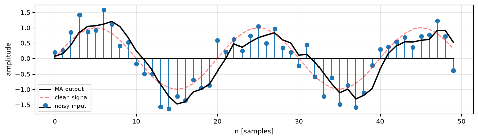
The code above uses scipy.signal.lfilter(b, a, x) to apply the filter. The b array holds the weights \([\tfrac{1}{3}, \tfrac{1}{3}, \tfrac{1}{3}]\), and a = [1] means there is no feedback. We’ll see what feedback means shortly.
Let’s step through the MA filter sample by sample to see exactly how it works. We assume all samples before \(n=0\) are zero (the signal “starts” at \(n=0\)):
x_short = np.array([-1, 2, 1, 0, 0, 0])
n_short = np.arange(len(x_short))

print(f"{'n':>3s}  {'x[n]':>6s}  {'x[n-1]':>7s}  {'x[n-2]':>7s}  {'y[n]':>8s}")
print("-" * 38)
for i in range(len(x_short)):
    xn = x_short[i]
    xn1 = x_short[i - 1] if i >= 1 else 0
    xn2 = x_short[i - 2] if i >= 2 else 0
    yn = (xn + xn1 + xn2) / 3
    print(f"{i:3d}  {xn:6.1f}  {xn1:7.1f}  {xn2:7.1f}  {yn:8.3f}")
n x[n] x[n-1] x[n-2] y[n]
--------------------------------------
0 -1.0 0.0 0.0 -0.333
1 2.0 -1.0 0.0 0.333
2 1.0 2.0 -1.0 0.667
3 0.0 1.0 2.0 1.000
4 0.0 0.0 1.0 0.333
5 0.0 0.0 0.0 0.000Notice how the output is a “smeared” version of the input: the impulse at \(n=1\) spreads across three output samples. This spreading is exactly what convolution does.
The general difference equation
The moving average is a specific example of a much broader family. Any discrete-time filter can be described by a difference equation that relates the output \(y[n]\) to past and present values of both the input \(x[n]\) and the output itself:
\[y[n] = \sum_{i=0}^{P} b_i\, x[n-i] \;-\; \sum_{j=1}^{Q} a_j\, y[n-j]\]
where:
- \(b_0, b_1, \ldots, b_P\) are the feedforward coefficients (they weight current and past inputs)
- \(a_1, a_2, \ldots, a_Q\) are the feedback coefficients (they weight past outputs)
- \(P\) is the feedforward order, \(Q\) is the feedback order
Our 3-point MA filter is a special case with \(b_0 = b_1 = b_2 = \tfrac{1}{3}\) and all feedback coefficients equal to zero.
If all the \(a_j\) are zero (no feedback), the filter depends only on the input: it is a finite impulse response (FIR) filter. The MA filter is FIR. If any \(a_j \neq 0\), the output feeds back into itself: it is an infinite impulse response (IIR) filter.
Exercise: Identify the coefficients
A filter is described by: \(y[n] = 0.5\,x[n] + 0.3\,x[n-1] + 0.2\,x[n-2]\)
What are the feedforward coefficients \(b_i\)? Is this FIR or IIR? What is its order?
Answer
\(b = [0.5, 0.3, 0.2]\), no feedback coefficients → FIR, order 2. Note that the coefficients sum to 1.0, so this filter preserves the DC level (like a weighted average).
Impulse response
The impulse response \(h[n]\) is the output of a system when the input is a Kronecker delta \(\delta[n]\), a single unit impulse at \(n=0\).
For an LTI system, the impulse response tells you everything about the system. Any input can be decomposed into shifted and scaled impulses (as we saw in Chapter 1), and by linearity and time-invariance, the output is the sum of shifted and scaled impulse responses.
FIR impulse response
For an FIR filter, the impulse response is simply the filter coefficients themselves:
\[h[n] = \begin{cases} b_n & 0 \leq n \leq P \\ 0 & \text{otherwise} \end{cases}\]
The impulse response has finite length \(P+1\), hence the name “finite impulse response.”
b = np.array([1/3, 1/3, 1/3])  # MA coefficients
h = b  # FIR impulse response IS the coefficients

n_h = np.arange(len(h))
fig, ax = plt.subplots(figsize=(6, 3))
ax.stem(n_h, h, linefmt='k-', markerfmt='ko', basefmt='k-')
ax.set_xlabel('n [samples]')
ax.set_ylabel('h[n]')
ax.set_title('Impulse response of 3-point MA filter')
ax.set_ylim(-0.1, 0.5)
ax.grid(True, alpha=0.3)
plt.tight_layout()
plt.show()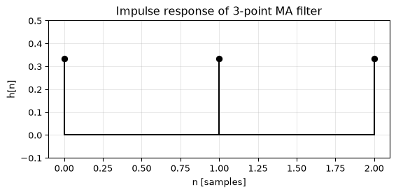
IIR impulse response
An IIR filter includes feedback, so its impulse response continues indefinitely. Consider a simple first-order IIR filter:
\[y[n] = x[n] + a \cdot y[n-1]\]
Sign convention
Compare this with the general form above: \(y[n] = \sum b_i\,x[n-i] - \sum a_j\,y[n-j]\). Writing the feedback gain as \(r\), we have \(b_0 = 1\) and \(a_1 = -r\). Substituting: \(y[n] = x[n] - (-r)\,y[n-1] = x[n] + r\,y[n-1]\). In Python’s scipy.signal.lfilter(b, a, x), the a vector is [1, -r], so the sign flip is baked in. See the exercise set for more practice with this convention.
When the input is \(\delta[n]\):
- \(h[0] = 1\) (the impulse passes through)
- \(h[1] = a \cdot h[0] = a\)
- \(h[2] = a \cdot h[1] = a^2\)
- In general: \(h[n] = a^n\) for \(n \geq 0\)
The impulse response is a decaying geometric sequence (if \(|a| < 1\)). It never reaches exactly zero: it has infinite duration.
fig, axes = plt.subplots(1, 3, figsize=(12, 3), sharey=True)
n_iir = np.arange(20)

for ax, a in zip(axes, [0.5, 0.9, -0.7]):
    h = a ** n_iir
    ax.stem(n_iir, h, linefmt='k-', markerfmt='ko', basefmt='k-')
    ax.set_xlabel('n')
    ax.set_title(f'a = {a}')
    ax.grid(True, alpha=0.3)
    ax.axhline(0, color='k', linewidth=0.5)

axes[0].set_ylabel('h[n]')
plt.suptitle('IIR impulse response: $h[n] = a^n \\cdot u[n]$', fontsize=11)
plt.tight_layout()
plt.show()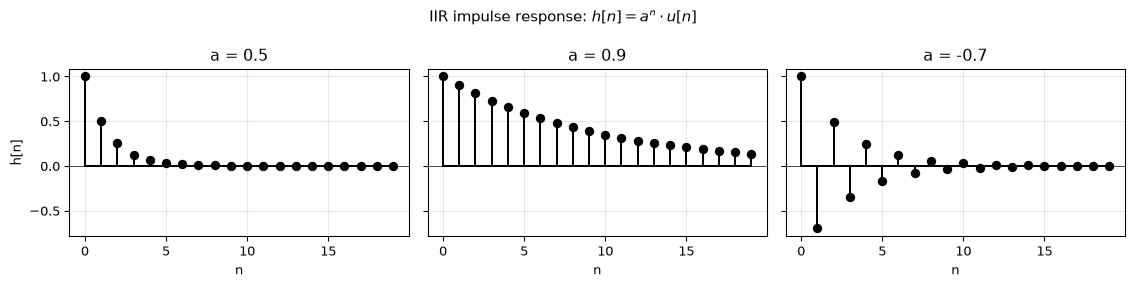
When \(|a| < 1\), the impulse response decays to zero: the system is stable. When \(|a| \geq 1\), the response grows without bound: the system is unstable. The sign of \(a\) determines whether the response alternates (negative \(a\)) or decays monotonically (positive \(a\)).
Convolution
The fundamental result of LTI system theory (Oppenheim and Schafer 2010): the output of any LTI system is the convolution of the input with the impulse response:
\[y[n] = x[n] * h[n] = \sum_{k=-\infty}^{\infty} h[k] \cdot x[n-k]\]
The * symbol denotes convolution (not multiplication). For causal systems (\(h[k] = 0\) for \(k < 0\)) with causal inputs (\(x[k] = 0\) for \(k < 0\)), the sum reduces to \(\sum_{k=0}^{n} h[k] \cdot x[n-k]\). The idea is: for each output sample \(y[n]\), flip the impulse response, slide it along the input, and sum the products.
Convolution is:
- Commutative: \(x * h = h * x\)
- Associative: \((x * h_1) * h_2 = x * (h_1 * h_2)\): cascading two filters is the same as convolving their impulse responses first
- Distributive: \(x * (h_1 + h_2) = x * h_1 + x * h_2\): parallel filters sum
x_conv = np.array([0, 0, 1, 2, -1, 0, 0])
h_conv = np.array([1/3, 1/3, 1/3])
y_conv = np.convolve(x_conv, h_conv)

fig, axes = plt.subplots(3, 1, figsize=(10, 6), sharex=True)

n_x = np.arange(len(x_conv))
n_y = np.arange(len(y_conv))

axes[0].stem(n_x, x_conv, linefmt='b-', markerfmt='bo', basefmt='k-')
axes[0].set_ylabel('x[n]')
axes[0].set_title('Input')
axes[0].grid(True, alpha=0.3)

axes[1].stem(np.arange(len(h_conv)), h_conv, linefmt='r-', markerfmt='ro', basefmt='k-')
axes[1].set_ylabel('h[n]')
axes[1].set_title('Impulse response (MA)')
axes[1].grid(True, alpha=0.3)

axes[2].stem(n_y, y_conv, linefmt='k-', markerfmt='ko', basefmt='k-')
axes[2].set_ylabel('y[n]')
axes[2].set_title('Output = x * h')
axes[2].set_xlabel('n [samples]')
axes[2].grid(True, alpha=0.3)

plt.tight_layout()
plt.show()

print(f"Input length:    {len(x_conv)}")
print(f"Impulse length:  {len(h_conv)}")
print(f"Output length:   {len(y_conv)}  (= {len(x_conv)} + {len(h_conv)} - 1)")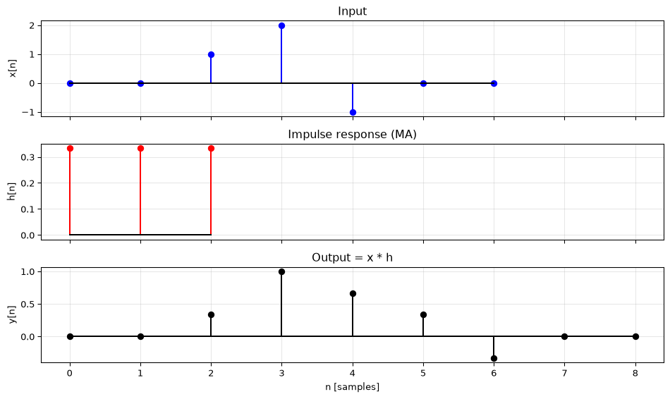
Input length:    7
Impulse length:  3
Output length:   9  (= 7 + 3 - 1)
The output length of a linear convolution is \(\text{len}(x) + \text{len}(h) - 1\).
Exercise: Convolution output length
A signal of length 100 is convolved with an impulse response of length 11. How long is the output? If the signal is sampled at 1000 Hz, how much extra time (in milliseconds) does the output span compared to the input?
Answer
Output length \(= 100 + 11 - 1 = 110\) samples. The extra 10 samples at 1000 Hz correspond to \(10/1000 = 10\) ms of additional duration. This “tail” is the filter’s transient ring-down.
In Python, np.convolve(x, h) computes this directly. For filtering long signals, scipy.signal.lfilter(b, a, x) is more efficient: it applies the difference equation sample by sample without materialising the full convolution.
FIR vs IIR: comparison
The two families of filters have complementary strengths:
| Property | FIR | IIR |
|---|---|---|
| Impulse response | Finite (length \(P+1\)) | Infinite (decaying) |
| Feedback | None | Required |
| Stability | Always stable | Can be unstable |
| Linear phase | Easy (symmetric coefficients) | Difficult (Bessel approximation) |
| Efficiency | More taps needed | Fewer coefficients |
| Difference equation | \(y[n] = \sum b_i\, x[n-i]\) | \(y[n] = \sum b_i\, x[n-i] - \sum a_j\, y[n-j]\) |
from scipy.signal import lfilter

np.random.seed(42)
n = np.arange(80)
x = np.sin(2 * np.pi * 0.04 * n) + 0.5 * np.random.randn(len(n))

# FIR: 5-point moving average
b_fir = np.ones(5) / 5
y_fir = lfilter(b_fir, [1], x)

# IIR: first-order lowpass (exponential smoothing)
alpha = 0.3
b_iir = [alpha]
a_iir = [1, -(1 - alpha)]
y_iir = lfilter(b_iir, a_iir, x)

fig, ax = plt.subplots(figsize=(10, 3))
ax.plot(n, x, 'C0-', alpha=0.3, label='noisy input')
ax.plot(n, y_fir, 'b-', linewidth=2, label='FIR (5-pt MA)')
ax.plot(n, y_iir, 'r-', linewidth=2, label=f'IIR (α={alpha})')
ax.set_xlabel('n [samples]')
ax.set_ylabel('amplitude')
ax.legend(fontsize=8)
ax.grid(True, alpha=0.3)
plt.tight_layout()
plt.show()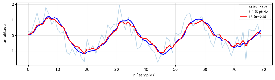
Both achieve smoothing, but the IIR filter uses only 2 coefficients where the FIR uses 5. The IIR filter introduces more phase delay (visible as a rightward shift), a trade-off we’ll revisit in the chapter on zero-phase filtering.
Causality and stability
Two properties determine whether a filter is practically useful.
Causality
A system is causal if the output at time \(n\) depends only on the current and past inputs, never on future values. For a causal system:
\[h[n] = 0 \quad \text{for } n < 0\]
All real-time systems must be causal (you can’t access future samples). When processing stored data offline, non-causal filters are possible and sometimes useful (zero-phase filtering exploits this).
BIBO stability
A system is BIBO stable (bounded-input, bounded-output) if every bounded input produces a bounded output (Oppenheim and Schafer 2010). For an LTI system, the necessary and sufficient condition is that the impulse response is absolutely summable:
\[\sum_{n=-\infty}^{\infty} |h[n]| < \infty\]
For FIR filters, this is always satisfied (finite sum of finite values). For IIR filters, stability depends on the feedback coefficients, or equivalently, on the locations of the system’s poles (which we’ll study in Chapter 4: The z-domain).
fig, axes = plt.subplots(1, 2, figsize=(10, 3))
n_stab = np.arange(30)

for ax, a, title in zip(axes, [0.8, 1.05], ['Stable (a=0.8)', 'Unstable (a=1.05)']):
    h = a ** n_stab
    ax.stem(n_stab, h, linefmt='k-', markerfmt='ko', basefmt='k-')
    ax.set_xlabel('n')
    ax.set_ylabel('h[n]')
    ax.set_title(title)
    ax.grid(True, alpha=0.3)

plt.tight_layout()
plt.show()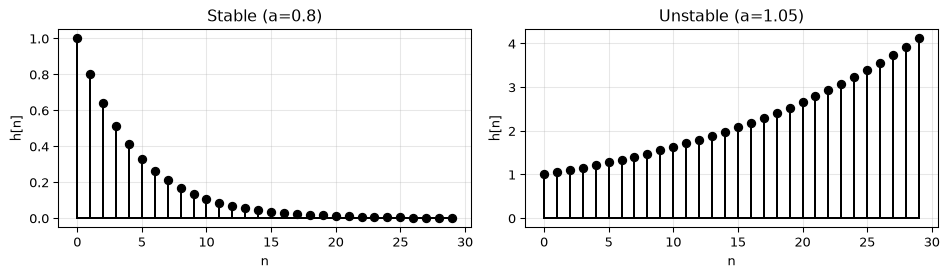
Summary
- A discrete-time system maps an input sequence to an output sequence.
- LTI systems (linear, time-invariant) are the central class, fully described by their impulse response.
- A difference equation relates the output to weighted sums of past inputs and past outputs.
- FIR filters (no feedback) have finite impulse responses, are always stable, and can have linear phase.
- IIR filters (with feedback) have infinite impulse responses, are more efficient, but can be unstable.
- Convolution \(y = x * h\) computes the output of any LTI system from the input and the impulse response.
- A system is causal if \(h[n] = 0\) for \(n < 0\), and BIBO stable if \(\sum |h[n]| < \infty\).
Want more practice? See the Exercise set for Chapter 2 for additional problems at varying difficulty levels.
Further reading
- Oppenheim & Schafer, Discrete-Time Signal Processing (2010), Ch. 2.1–2.4: LTI systems, convolution, stability
- Proakis & Manolakis, Digital Signal Processing (2007), Ch. 2.3–2.4: Difference equations, impulse response
Going deeper
The Topics section explores several applications of filters introduced here:
- Adaptive filtering: filters that adjust their coefficients in real time (LMS, NLMS, RLS)
- Matched filtering: the optimal FIR filter for detecting a known pulse shape in noise
- Outlier detection: using sliding-window filters to detect anomalous values
The next chapter covers noise, the decibel scale, and signal-to-noise ratio: Noise and SNR.
References
Oppenheim, Alan V., and Ronald W. Schafer. 2010. Discrete-Time Signal Processing. 3rd ed. Pearson.