Exercises: The Z-Domain

Practice problems for Chapter 4

These exercises accompany Chapter 4: The Z-Domain.

Key formulas for this chapter

Formula	Description
\(X(z) = \sum_{n=0}^{\infty} x[n]\,z^{-n}\)	Z-transform definition
\(H(z) = B(z)/A(z)\)	Transfer function from difference equation
Stability: all poles \(\lvert p_i\rvert < 1\)	Pole criterion for BIBO stability
\(a^n u[n] \leftrightarrow z/(z-a)\)	Key z-transform pair
\(\delta[n] \leftrightarrow 1\)	Unit impulse transform pair
\(H(z)/z = A/(z-p_1) + B/(z-p_2) + \ldots\)	Partial fraction expansion

Basic

Exercise 1: z-transform from the definition

Compute the z-transform of the following signals:

\(x[n] = 3\,\delta[n] - 2\,\delta[n-1] + \delta[n-4]\)
\(x[n] = [1, 0, -1, 2]\) (a 4-sample sequence starting at \(n = 0\))
\(x[n] = 5\,u[n]\) (a constant signal for \(n \geq 0\))

Solution

Using linearity and the delay property: \[X(z) = 3 - 2z^{-1} + z^{-4}\]
Directly from the definition: \[X(z) = 1 + 0\cdot z^{-1} - z^{-2} + 2z^{-3} = 1 - z^{-2} + 2z^{-3}\]
Using the unit step transform pair \(u[n] \leftrightarrow \frac{z}{z-1}\): \[X(z) = 5 \cdot \frac{z}{z-1} = \frac{5z}{z-1}\]

Exercise 2: Difference equation to transfer function

Derive the transfer function \(H(z) = Y(z)/X(z)\) for each filter:

\(y[n] = x[n] - x[n-2]\) (first difference of alternate samples)
\(y[n] = 0.5\,x[n] + 0.5\,x[n-1]\) (2-point moving average)
\(y[n] = x[n] + 0.9\,y[n-1]\) (first-order IIR lowpass)
\(y[n] = x[n] - x[n-1] + 0.8\,y[n-1] - 0.6\,y[n-2]\) (second-order IIR)

Solution

\(H(z) = 1 - z^{-2} = \frac{z^2 - 1}{z^2}\). FIR, order 2.
\(H(z) = 0.5 + 0.5z^{-1} = \frac{z + 1}{2z}\). FIR, order 1.
\(Y(z)(1 - 0.9z^{-1}) = X(z)\), so \(H(z) = \frac{1}{1 - 0.9z^{-1}} = \frac{z}{z - 0.9}\). IIR, one pole at \(z = 0.9\).
\(Y(z)(1 - 0.8z^{-1} + 0.6z^{-2}) = X(z)(1 - z^{-1})\), so: \[H(z) = \frac{1 - z^{-1}}{1 - 0.8z^{-1} + 0.6z^{-2}} = \frac{z^2 - z}{z^2 - 0.8z + 0.6}\]

Exercise 3: Reading pole-zero plots

A filter has zeros at \(z = 1\) and \(z = -1\), and poles at \(z = 0.5\) and \(z = -0.5\). The gain is \(K = 1\).

Write the transfer function in factored form.
Is the system stable?
What is the filter order?

Solution

\(H(z) = \frac{(z-1)(z+1)}{(z-0.5)(z+0.5)} = \frac{z^2 - 1}{z^2 - 0.25}\)
Both poles have magnitude \(|p| = 0.5 < 1\), so yes, the system is stable.
The denominator is second-order, so it is a second-order filter.

Exercise 4: Stability check

For each transfer function, determine the poles and state whether the system is stable, marginally stable, or unstable.

\(H(z) = \frac{z}{z - 0.99}\)
\(H(z) = \frac{z + 1}{z^2 + 1}\)
\(H(z) = \frac{1}{z^2 - 1.5z + 0.56}\)

Solution

Pole at \(z = 0.99\). \(|0.99| < 1\) → stable (barely, close to the unit circle).
Poles where \(z^2 + 1 = 0\), i.e. \(z = \pm j\). Both have \(|z| = 1\) → marginally stable.
Poles from the quadratic formula: \(z = \frac{1.5 \pm \sqrt{2.25 - 2.24}}{2} = \frac{1.5 \pm 0.1}{2}\), giving \(z = 0.80\) and \(z = 0.70\). Both \(< 1\) → stable.

import numpy as np
from scipy.signal import tf2zpk

# Verify part (c)
z, p, k = tf2zpk([1], [1, -1.5, 0.56])
print(f"Poles: {p}")
print(f"|poles|: {np.abs(p)}")

Poles: [0.8 0.7]
|poles|: [0.8 0.7]

Intermediate

Exercise 5: Inverse z-transform

Find the impulse response \(h[n]\) for each transfer function, then verify with Python.

\(H(z) = \frac{z}{z - 0.8}\)
\(H(z) = 2 - 3z^{-1} + z^{-3}\)
\(H(z) = \frac{z}{z - 0.5} - \frac{z}{z + 0.5}\)

Solution

From the table: \(h[n] = 0.8^n\,u[n]\) (geometric decay).
Direct readoff (FIR): \(h[n] = 2\,\delta[n] - 3\,\delta[n-1] + \delta[n-3]\), i.e. \(h = [2, -3, 0, 1]\).
Using linearity: \(h[n] = (0.5)^n\,u[n] - (-0.5)^n\,u[n]\). For even \(n\) the terms cancel; for odd \(n\) they reinforce. So \(h[n] = 0\) for even \(n\) and \(h[n] = 2 \cdot (0.5)^n\) for odd \(n\).

import numpy as np
from scipy.signal import lfilter

n = np.arange(10)
delta = np.zeros(10); delta[0] = 1

# Part (a)
h_a = lfilter([1], [1, -0.8], delta)
h_a_formula = 0.8 ** n
print("(a) lfilter:", np.round(h_a, 4))
print("    formula:", np.round(h_a_formula, 4))

# Part (c) — combine two first-order sections
h_c1 = lfilter([1], [1, -0.5], delta)
h_c2 = lfilter([1], [1, 0.5], delta)
h_c = h_c1 - h_c2
h_c_formula = 0.5**n - (-0.5)**n
print("\n(c) lfilter:", np.round(h_c, 4))
print("    formula:", np.round(h_c_formula, 4))

(a) lfilter: [1.     0.8    0.64   0.512  0.4096 0.3277 0.2621 0.2097 0.1678 0.1342]
    formula: [1.     0.8    0.64   0.512  0.4096 0.3277 0.2621 0.2097 0.1678 0.1342]

(c) lfilter: [0.     1.     0.     0.25   0.     0.0625 0.     0.0156 0.     0.0039]
    formula: [0.     1.     0.     0.25   0.     0.0625 0.     0.0156 0.     0.0039]

Exercise 6: Pole placement for a resonator

A second-order resonator has complex conjugate poles at \(z = r\,e^{\pm j\omega_0}\) and zeros at the origin:

\[H(z) = \frac{1}{1 - 2r\cos(\omega_0)\,z^{-1} + r^2\,z^{-2}}\]

For \(\omega_0 = \pi/4\) and \(r = 0.9\), compute the pole locations and verify the system is stable.
What happens to the impulse response as \(r \to 1\)?
Write Python code to plot the pole-zero map and impulse response for \(r = 0.9\) and \(r = 0.99\).

Solution

The poles are at \(z = 0.9\,e^{\pm j\pi/4} = 0.9(\cos\frac{\pi}{4} \pm j\sin\frac{\pi}{4}) \approx 0.636 \pm 0.636j\). Both have magnitude \(|z| = 0.9 < 1\) → stable.
As \(r \to 1\), the poles approach the unit circle. The impulse response decays more slowly (longer ringing). At \(r = 1\), the system is marginally stable. The impulse response oscillates forever.

import numpy as np
import matplotlib.pyplot as plt
from scipy.signal import lfilter, tf2zpk

omega_0 = np.pi / 4
fig, axes = plt.subplots(2, 2, figsize=(10, 8))

for col, r in enumerate([0.9, 0.99]):
    b = [1]
    a = [1, -2*r*np.cos(omega_0), r**2]

    # Pole-zero plot
    z, p, k = tf2zpk(b, a)
    theta = np.linspace(0, 2*np.pi, 200)
    ax = axes[0, col]
    ax.plot(np.cos(theta), np.sin(theta), 'k-', linewidth=0.8, alpha=0.5)
    ax.plot(p.real, p.imag, 'rx', markersize=10, markeredgewidth=2)
    ax.axhline(0, color='k', linewidth=0.5)
    ax.axvline(0, color='k', linewidth=0.5)
    ax.set_aspect('equal')
    ax.set_title(f'Poles (r = {r})')
    ax.grid(True, alpha=0.3)

    # Impulse response
    n = np.arange(100)
    delta = np.zeros(100); delta[0] = 1
    h = lfilter(b, a, delta)
    axes[1, col].plot(n, h, 'k-', linewidth=0.7)
    axes[1, col].set_xlabel('n')
    axes[1, col].set_ylabel('h[n]')
    axes[1, col].set_title(f'Impulse response (r = {r})')
    axes[1, col].grid(True, alpha=0.3)

fig.tight_layout()
plt.show()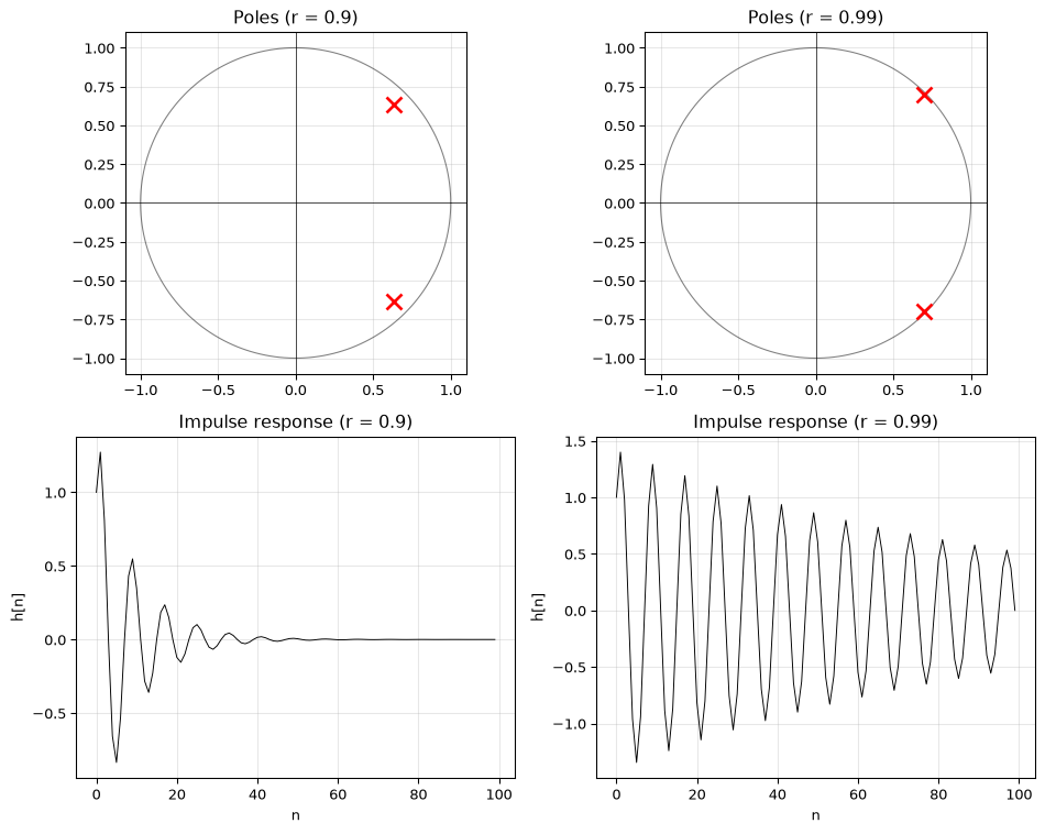

Exercise 7: Cascade of two filters

Two filters are connected in series (cascade): the output of the first is the input of the second.

Filter 1: \(H_1(z) = 1 + z^{-1}\) (2-point sum)

Filter 2: \(H_2(z) = 1 - z^{-1}\) (2-point difference)

What is the overall transfer function \(H(z) = H_1(z) \cdot H_2(z)\)?
What type of filter is the result? Is it FIR or IIR?
What is the impulse response of the cascade?

Solution

\(H(z) = (1 + z^{-1})(1 - z^{-1}) = 1 - z^{-2} = \frac{z^2 - 1}{z^2}\)
FIR, order 2. The cascade of two FIR filters is always FIR.
\(h[n] = \delta[n] - \delta[n-2]\), so \(h = [1, 0, -1]\). The cascade computes the difference between the current sample and the one two steps ago.

import numpy as np
from scipy.signal import lfilter

delta = np.zeros(6); delta[0] = 1

# Cascade: apply H1 then H2
y1 = lfilter([1, 1], [1], delta)   # H1
y2 = lfilter([1, -1], [1], y1)     # H2

# Direct: H = H1 * H2
y_direct = lfilter([1, 0, -1], [1], delta)

print("Cascade:", y2)
print("Direct: ", y_direct)

Cascade: [ 1.  0. -1.  0.  0.  0.]
Direct:  [ 1.  0. -1.  0.  0.  0.]

Challenge

Exercise 8: Design a notch filter from poles and zeros

A notch filter removes a single frequency. To null out frequency \(\omega_0\), place zeros on the unit circle at \(z = e^{\pm j\omega_0}\).

Write the transfer function for a notch filter at \(\omega_0 = \pi/4\) (zeros only, no poles beyond the origin).
Add poles at \(z = r\,e^{\pm j\omega_0}\) with \(r = 0.9\) to control the notch width. Write the new \(H(z)\).
Plot the pole-zero map and the impulse response for both versions. What effect do the poles have?

Solution

Zeros at \(e^{\pm j\pi/4}\): \[H(z) = (z - e^{j\pi/4})(z - e^{-j\pi/4}) = z^2 - 2\cos(\pi/4)\,z + 1 = z^2 - \sqrt{2}\,z + 1\]

In coefficient form: \(b = [1, -\sqrt{2}, 1]\), \(a = [1]\).

With poles at \(r = 0.9\): \[H(z) = \frac{z^2 - \sqrt{2}\,z + 1}{z^2 - 0.9\sqrt{2}\,z + 0.81}\]

\(b = [1, -\sqrt{2}, 1]\), \(a = [1, -0.9\sqrt{2}, 0.81]\).

import numpy as np
import matplotlib.pyplot as plt
from scipy.signal import lfilter, tf2zpk

omega_0 = np.pi / 4
r = 0.9

fig, axes = plt.subplots(2, 2, figsize=(10, 8))
theta = np.linspace(0, 2*np.pi, 200)

configs = [
    ('FIR notch (zeros only)', [1, -np.sqrt(2), 1], [1]),
    ('IIR notch (with poles)', [1, -np.sqrt(2), 1], [1, -r*np.sqrt(2), r**2]),
]

for col, (title, b, a) in enumerate(configs):
    z, p, k = tf2zpk(b, a)

    # Pole-zero plot
    ax = axes[0, col]
    ax.plot(np.cos(theta), np.sin(theta), 'k-', linewidth=0.8, alpha=0.5)
    if len(z) > 0:
        ax.plot(z.real, z.imag, 'bo', markersize=10, markerfacecolor='none', markeredgewidth=2)
    if len(p) > 0:
        ax.plot(p.real, p.imag, 'rx', markersize=10, markeredgewidth=2)
    ax.axhline(0, color='k', linewidth=0.5)
    ax.axvline(0, color='k', linewidth=0.5)
    ax.set_aspect('equal')
    ax.set_title(title)
    ax.grid(True, alpha=0.3)

    # Impulse response
    n = np.arange(40)
    delta = np.zeros(40); delta[0] = 1
    h = lfilter(b, a, delta)
    axes[1, col].stem(n, h, linefmt='k-', markerfmt='k.', basefmt='k-')
    axes[1, col].set_xlabel('n')
    axes[1, col].set_ylabel('h[n]')
    axes[1, col].set_title('Impulse response')
    axes[1, col].grid(True, alpha=0.3)

fig.tight_layout()
plt.show()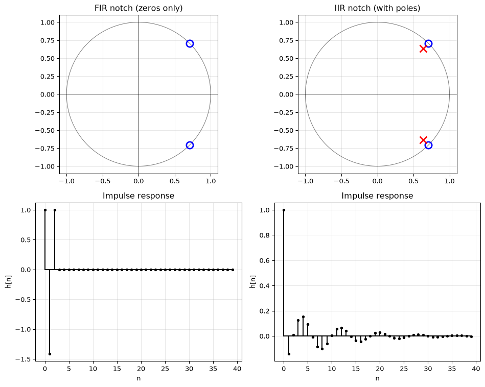

The FIR version (zeros only) has a 3-tap impulse response, which is very short but the notch is broad. Adding poles near the zeros narrows the notch, giving a more selective filter, at the cost of a longer (theoretically infinite) impulse response.

Exercise 9: Stability boundary exploration

Consider the family of second-order filters:

\[H(z) = \frac{1}{1 + a_1\,z^{-1} + a_2\,z^{-2}}\]

For \(a_1 = 0\) and varying \(a_2\), what is the stability condition?
Write Python code that sweeps \(a_1 \in [-2, 2]\) and \(a_2 \in [-1, 1]\) and plots the stability triangle: the region of \((a_1, a_2)\) where the system is stable.

Solution

With \(a_1 = 0\): poles at \(z^2 + a_2 = 0\), so \(z = \pm\sqrt{-a_2}\).

If \(a_2 < 0\): real poles at \(\pm\sqrt{|a_2|}\). Stable when \(|a_2| < 1\), i.e. \(-1 < a_2 < 0\).
If \(a_2 > 0\): imaginary poles at \(\pm j\sqrt{a_2}\). Stable when \(\sqrt{a_2} < 1\), i.e. \(0 < a_2 < 1\).
Combined: stable when \(|a_2| < 1\).

import numpy as np
import matplotlib.pyplot as plt
from matplotlib.patches import Polygon

a1_range = np.linspace(-2.5, 2.5, 500)
a2_range = np.linspace(-1.5, 1.5, 500)
A1, A2 = np.meshgrid(a1_range, a2_range)

# For each (a1, a2), compute max pole magnitude
# Denominator: z^2 + a1*z + a2 = 0
# Poles: z = (-a1 ± sqrt(a1^2 - 4*a2)) / 2
discriminant = A1**2 - 4*A2
# Max pole magnitude
z1 = (-A1 + np.sqrt(discriminant.astype(complex))) / 2
z2 = (-A1 - np.sqrt(discriminant.astype(complex))) / 2
max_pole = np.maximum(np.abs(z1), np.abs(z2))

fig, ax = plt.subplots(figsize=(7, 5))
stable = (max_pole < 1).astype(float)
ax.contourf(A1, A2, stable, levels=[0.5, 1.5], colors=['#c8e6c9'], alpha=0.7)
ax.contour(A1, A2, stable, levels=[0.5], colors=['green'], linewidths=2)

# The stability triangle has vertices at (-2,1), (2,1), (0,-1)
triangle = Polygon([(-2, 1), (2, 1), (0, -1)], fill=False,
                   edgecolor='red', linestyle='--', linewidth=1.5, label='Stability triangle')
ax.add_patch(triangle)

ax.set_xlabel('$a_1$')
ax.set_ylabel('$a_2$')
ax.set_title('Stability region for second-order IIR filters')
ax.legend()
ax.grid(True, alpha=0.3)
ax.set_xlim(-2.5, 2.5)
ax.set_ylim(-1.5, 1.5)
fig.tight_layout()
plt.show()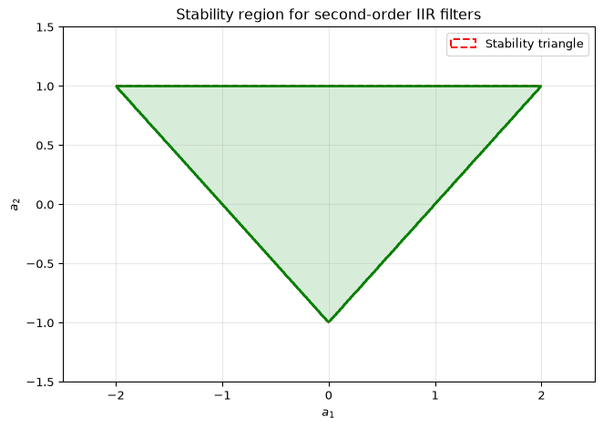

The stable region is a triangle with vertices at \((-2, 1)\), \((2, 1)\), and \((0, -1)\). The three edges correspond to the conditions: \(a_2 < 1\), \(a_2 > a_1 - 1\), and \(a_2 > -a_1 - 1\). This is the classic stability triangle for second-order IIR filters.

Exercise 10: Identify the system from its impulse response (Basic)

The table below gives the first ten samples of an unknown system’s impulse response \(h[n]\):

\(n\)	0	1	2	3	4	5	6	7	8	9
\(h[n]\)	1.000	0.700	0.490	0.343	0.240	0.168	0.118	0.082	0.058	0.040

The values decrease geometrically. Estimate the ratio \(h[n+1]/h[n]\) and use it to identify the pole.
Write down the transfer function \(H(z)\) and the difference equation.
Is the system FIR or IIR? Stable or unstable?

Solution

Each sample is \(0.7\) times the previous: \(h[1]/h[0] = 0.7\), \(h[2]/h[1] = 0.49/0.7 = 0.7\), etc. The decay ratio is \(0.7\), indicating a single real pole at \(z = 0.7\).
For a first-order IIR with pole at \(p = 0.7\) and \(h[0] = 1\): \[H(z) = \frac{1}{1 - 0.7\,z^{-1}} = \frac{z}{z - 0.7}\] Difference equation: \(y[n] = x[n] + 0.7\,y[n-1]\).
IIR (the impulse response never reaches zero exactly). Stable, because \(|0.7| < 1\).

import numpy as np
from scipy.signal import lfilter

h_data = np.array([1.000, 0.700, 0.490, 0.343, 0.240,
                   0.168, 0.118, 0.082, 0.058, 0.040])

# Estimate ratio from successive samples
ratios = h_data[1:] / h_data[:-1]
print(f"Sample ratios: {np.round(ratios, 4)}")
print(f"Mean ratio (estimated pole): {np.mean(ratios):.4f}")

# Verify: simulate H(z) = 1/(1 - 0.7 z^{-1})
delta = np.zeros(10); delta[0] = 1
h_sim = lfilter([1], [1, -0.7], delta)
print(f"\nSimulated h[n]: {np.round(h_sim, 4)}")
print(f"Data matches:   {np.allclose(h_data, h_sim, atol=1e-3)}")

Sample ratios: [0.7    0.7    0.7    0.6997 0.7    0.7024 0.6949 0.7073 0.6897]
Mean ratio (estimated pole): 0.6993

Simulated h[n]: [1.     0.7    0.49   0.343  0.2401 0.1681 0.1176 0.0824 0.0576 0.0404]
Data matches:   True

Exercise 11: Debug this: pole-zero plot code (Basic)

A student writes the following code to plot the pole-zero diagram of the filter:

\[H(z) = \frac{z^2 - 1}{z^2 - 0.5z + 0.5}\]

import numpy as np
import matplotlib.pyplot as plt
from scipy.signal import tf2zpk

# Numerator and denominator in z^{-1} powers
b = [1, 0, -1]         # 1 - z^{-2}
a = [1, -0.5, 0.5]     # 1 - 0.5 z^{-1} + 0.5 z^{-2}

z, p, k = tf2zpk(b, a)

theta = np.linspace(0, 2*np.pi, 200)
plt.figure()
plt.plot(np.cos(theta), np.sin(theta), 'k-')
plt.plot(z.real, z.imag, 'bx', markersize=10)   # zeros
plt.plot(p.real, p.imag, 'ro', markersize=10)    # poles
plt.axis('equal')
plt.grid(True)
plt.title('Pole-zero plot')
plt.show()

There is one bug that makes the plot wrong, and one misleading comment. Find and fix both.

Solution

Bug (wrong plot): The markers for zeros and poles are swapped. Convention: zeros → circles ('o'), poles → crosses ('x'). The code has it backwards.

Misleading comment: The comment says “in \(z^{-1}\) powers” but tf2zpk expects coefficients in descending powers of \(z\). For this transfer function the arrays happen to be the same either way, so the computed values are correct, but the comment should be fixed to avoid confusion on asymmetric polynomials.

Fixed code:

import numpy as np
import matplotlib.pyplot as plt
from scipy.signal import tf2zpk

b = [1, 0, -1]       # z^2 - 1
a = [1, -0.5, 0.5]   # z^2 - 0.5z + 0.5

z, p, k = tf2zpk(b, a)
print(f"Zeros: {np.round(z, 4)}")
print(f"Poles: {np.round(p, 4)}")
print(f"|poles|: {np.round(np.abs(p), 4)}  (< 1 → stable)")

theta = np.linspace(0, 2*np.pi, 200)
plt.figure(figsize=(5, 5))
plt.plot(np.cos(theta), np.sin(theta), 'k-', linewidth=0.8, alpha=0.5)
plt.plot(z.real, z.imag, 'bo', markersize=12,           # zeros: circles
         markerfacecolor='none', markeredgewidth=2, label='Zeros')
plt.plot(p.real, p.imag, 'rx', markersize=12,            # poles: crosses
         markeredgewidth=2, label='Poles')
plt.axhline(0, color='k', linewidth=0.5)
plt.axvline(0, color='k', linewidth=0.5)
plt.axis('equal')
plt.grid(True, alpha=0.3)
plt.legend()
plt.title('Pole-zero plot (corrected)')
plt.tight_layout()
plt.show()

Zeros: [-1.  1.]
Poles: [0.25+0.6614j 0.25-0.6614j]
|poles|: [0.7071 0.7071]  (< 1 → stable)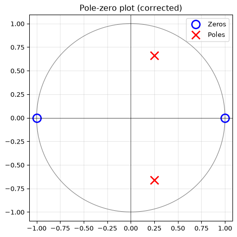

Exercise 12: Which filter is unstable? (Basic)

Four IIR filters are defined by their denominator coefficients \(a\) (with \(a[0] = 1\)). Without running any code, decide which are stable and which are unstable.

Filter	\(a\) coefficients
A	`[1, -0.5, 0.25]`
B	`[1, 1.0, 0.9]`
C	`[1, -1.5, 1.0]`
D	`[1, -0.5, 1.2]`

Check your answers in Python.

Solution

Compute the poles for each denominator \(z^2 + a_1 z + a_2 = 0\):

Filter A: \(a_1 = -0.5\), \(a_2 = 0.25\). Discriminant \(= 0.25 - 1 < 0\): complex poles. \(|p|^2 = a_2 = 0.25\), so \(|p| = 0.5 < 1\) → stable.

Filter B: \(a_1 = 1.0\), \(a_2 = 0.9\). \(|p|^2 = 0.9 < 1\) (complex poles since discriminant \(= 1 - 3.6 < 0\)) → stable.

Filter C: \(a_1 = -1.5\), \(a_2 = 1.0\). \(|p|^2 = 1.0\): poles on the unit circle → marginally stable.

Filter D: \(a_1 = -0.5\), \(a_2 = 1.2\). \(|p|^2 = a_2 = 1.2 > 1\): poles outside the unit circle → unstable.

import numpy as np
from scipy.signal import tf2zpk

filters = {
    'A': ([1], [1, -0.5,  0.25]),
    'B': ([1], [1,  1.0,  0.90]),
    'C': ([1], [1, -1.5,  1.00]),
    'D': ([1], [1, -0.5,  1.20]),
}

for name, (b, a) in filters.items():
    _, p, _ = tf2zpk(b, a)
    max_mag = np.max(np.abs(p))
    if max_mag < 1:
        verdict = 'stable'
    elif np.isclose(max_mag, 1.0, atol=1e-9):
        verdict = 'marginally stable'
    else:
        verdict = 'UNSTABLE'
    print(f"Filter {name}: poles = {np.round(p, 4)}, |p|_max = {max_mag:.4f} → {verdict}")

Filter A: poles = [0.25+0.433j 0.25-0.433j], |p|_max = 0.5000 → stable
Filter B: poles = [-0.5+0.8062j -0.5-0.8062j], |p|_max = 0.9487 → stable
Filter C: poles = [0.75+0.6614j 0.75-0.6614j], |p|_max = 1.0000 → marginally stable
Filter D: poles = [0.25+1.0665j 0.25-1.0665j], |p|_max = 1.0954 → UNSTABLE

Intermediate (continued)

Exercise 13: Estimate decay time from pole radius (Intermediate)

A first-order IIR filter has a real pole at \(z = r\) (\(0 < r < 1\)). Its impulse response is \(h[n] = r^n\,u[n]\).

Derive a formula for \(N_{60}\), the number of samples it takes for \(h[n]\) to fall to \(1/1000\) of its initial value (approximately \(-60\,\text{dB}\)).
Use your formula to fill in the table:

\(r\)	\(N_{60}\) (formula)
0.5
0.9
0.99
0.999

A system sampled at \(f_s = 8000\,\text{Hz}\) must have a \(-60\,\text{dB}\) decay time shorter than \(10\,\text{ms}\). What is the maximum allowed pole radius?

Solution

We want \(r^N = 10^{-3}\), so: \[N_{60} = \frac{-3 \ln 10}{\ln r} = \frac{3 \ln 10}{-\ln r} \approx \frac{6.908}{-\ln r}\]

\(r\)	\(N_{60}\) (formula)
0.5	\(6.908 / 0.693 \approx 10\)
0.9	\(6.908 / 0.105 \approx 66\)
0.99	\(6.908 / 0.01005 \approx 687\)
0.999	\(6.908 / 0.001 \approx 6908\)

At \(f_s = 8000\,\text{Hz}\), \(10\,\text{ms}\) corresponds to \(0.010 \times 8000 = 80\) samples. We need \(N_{60} \leq 80\): \[\frac{6.908}{-\ln r} \leq 80 \implies -\ln r \geq \frac{6.908}{80} \implies r \leq e^{-0.08635} \approx 0.917\]

import numpy as np

def N60(r):
    return 3 * np.log(10) / (-np.log(r))

print("Decay table:")
for r in [0.5, 0.9, 0.99, 0.999]:
    print(f"  r = {r:.3f}:  N_60 = {N60(r):.1f} samples")

# Part (c)
fs = 8000
t_limit = 0.010          # 10 ms
n_limit = t_limit * fs   # 80 samples
r_max = np.exp(-3 * np.log(10) / n_limit)
print(f"\nMax pole radius for N_60 ≤ {n_limit:.0f} samples: r ≤ {r_max:.4f}")

# Verify: N_60 at r_max should equal 80
print(f"Check: N_60(r_max) = {N60(r_max):.1f} samples")

Decay table:
  r = 0.500:  N_60 = 10.0 samples
  r = 0.900:  N_60 = 65.6 samples
  r = 0.990:  N_60 = 687.3 samples
  r = 0.999:  N_60 = 6904.3 samples

Max pole radius for N_60 ≤ 80 samples: r ≤ 0.9173
Check: N_60(r_max) = 80.0 samples

Exercise 14: Debug this: partial fraction decomposition (Intermediate)

A student decomposes the following transfer function using partial fractions and makes an error:

\[H(z) = \frac{z}{(z - 0.5)(z - 0.8)}\]

Student’s working:

\[\frac{H(z)}{z} = \frac{1}{(z-0.5)(z-0.8)} = \frac{A}{z - 0.5} + \frac{B}{z - 0.8}\]

\[A = \left.\frac{1}{z - 0.8}\right|_{z=0.5} = \frac{1}{0.5 - 0.8} = \frac{1}{-0.3} \approx -3.33\]

\[B = \left.\frac{1}{z - 0.5}\right|_{z=0.5} = \frac{1}{0.8 - 0.5} = \frac{1}{0.3} \approx 3.33\]

\[\therefore h[n] = -3.33\,(0.5)^n\,u[n] + 3.33\,(0.8)^n\,u[n]\]

Identify the error in the student’s computation of \(B\).
State the correct value of \(B\) and the correct impulse response.
Verify numerically that the correct \(h[n]\) matches the output of scipy.signal.lfilter.

Solution

The student evaluated \(B\) at \(z = 0.5\) instead of at the pole \(z = 0.8\). The cover-up rule for \(B\) requires setting \(z = 0.8\) (the pole of the \(B\) term), not \(z = 0.5\).
Correct calculation: \[B = \left.\frac{1}{z - 0.5}\right|_{z=0.8} = \frac{1}{0.8 - 0.5} = \frac{1}{0.3} \approx 3.33\]

In this case the numerical value of \(B\) is the same as the student wrote, but only by coincidence of the symmetric denominator values. The correct residues are \(A \approx -3.33\) and \(B \approx 3.33\), giving:

\[h[n] = \left[-3.33\,(0.5)^n + 3.33\,(0.8)^n\right]u[n]\]

The student’s formula happened to be correct here, but the method was wrong, and it would fail for any asymmetric pole pair.

import numpy as np
from scipy.signal import lfilter, residuez

# H(z) = z / ((z-0.5)(z-0.8)) = z / (z^2 - 1.3z + 0.4)
# In z^{-1} form: divide by z^2 → H(z) = z^{-1} / (1 - 1.3z^{-1} + 0.4z^{-2})
# lfilter uses z^{-1} coefficients: b = [0, 1] for z^{-1}, a = [1, -1.3, 0.4]
b = [0, 1]          # z^{-1}  (numerator is a pure one-sample delay)
a = [1, -1.3, 0.4]  # 1 - 1.3z^{-1} + 0.4z^{-2}

# Partial fractions via residuez (works in z^{-1} domain)
r, pol, k = residuez(b, a)
print("Residues:", np.round(r, 4))
print("Poles:   ", np.round(pol, 4))

# Manual formula
n = np.arange(15)
h_formula = (-10/3) * (0.5**n) + (10/3) * (0.8**n)

# Exact residues: A = 1/(0.5-0.8)=-10/3, B = 1/(0.8-0.5)=10/3
print(f"\nExact A = {1/(0.5-0.8):.6f}")
print(f"Exact B = {1/(0.8-0.5):.6f}")

# Simulate with lfilter
delta = np.zeros(15); delta[0] = 1
h_filter = lfilter(b, a, delta)

print("\nn | h_formula | h_lfilter")
for i in range(8):
    print(f"{i} | {h_formula[i]:.4f}     | {h_filter[i]:.4f}")
print(f"Match: {np.allclose(h_formula, h_filter, atol=1e-6)}")

Residues: [-3.3333  3.3333]
Poles:    [0.5 0.8]

Exact A = -3.333333
Exact B = 3.333333

n | h_formula | h_lfilter
0 | 0.0000     | 0.0000
1 | 1.0000     | 1.0000
2 | 1.3000     | 1.3000
3 | 1.2900     | 1.2900
4 | 1.1570     | 1.1570
5 | 0.9881     | 0.9881
6 | 0.8217     | 0.8217
7 | 0.6730     | 0.6730
Match: True

Exercise 15: DC blocker: analyse a given filter (Intermediate)

The one-pole DC blocker is defined by:

\[H(z) = \frac{1 - z^{-1}}{1 - r\,z^{-1}}, \quad r = 0.995\]

Locate the zero and the pole. Explain why this filter blocks DC (zero frequency).
Write the difference equation. What is the computational cost in multiply-accumulate operations per sample?
The code below computes the frequency response but produces a response with the null at the wrong frequency (near Nyquist instead of DC). Find and fix the bug.

import numpy as np
import matplotlib.pyplot as plt

r = 0.995
b = [1, -1]
a = [1, r]        # Bug is here

w = np.linspace(0, np.pi, 512)
H = np.polyval(b, np.exp(1j*w)) / np.polyval(a, np.exp(1j*w))
plt.plot(w / np.pi, 20*np.log10(np.abs(H)))
plt.xlabel('Normalised frequency')
plt.ylabel('Magnitude (dB)')
plt.show()

Solution

Zero at \(z = 1\) (DC, \(\omega = 0\)): the numerator \((1 - z^{-1})\) vanishes at \(z = 1\). Pole at \(z = r = 0.995\), just inside the unit circle. The pole is close to the zero, so it partially “cancels” the zero’s effect away from DC, leaving frequencies above DC relatively unattenuated.
Difference equation: \(y[n] = x[n] - x[n-1] + r\,y[n-1]\). Cost: 1 multiplication and 2 additions per sample (extremely cheap).
The bug is in the denominator coefficient sign. The denominator in \(z^{-1}\) form is \(1 - r\,z^{-1}\), but the code writes a = [1, r] (positive \(r\)), which implements \(1 + r\,z^{-1}\), giving a pole at \(z = -r\) instead of \(z = +r\). Fix: a = [1, -r].

import numpy as np
import matplotlib.pyplot as plt

from scipy.signal import freqz

r = 0.995
b = [1, -1]
a_fixed = [1, -r]   # corrected: was [1, r]

w_plot, H = freqz(b, a_fixed, worN=2048)

plt.figure(figsize=(7, 3))
plt.plot(w_plot / np.pi, 20*np.log10(np.abs(H) + 1e-12), 'k-')
plt.xlabel('Normalised frequency ($\\times \\pi$ rad/sample)')
plt.ylabel('Magnitude (dB)')
plt.title('DC blocker frequency response (corrected)')
plt.ylim(-80, 5)
plt.grid(True, alpha=0.3)
plt.tight_layout()
plt.show()

# Show the zero and pole
from scipy.signal import tf2zpk
z, p, k = tf2zpk(b, a_fixed)
print(f"Zero: {z}  (|z| = {np.abs(z[0]):.3f})")
print(f"Pole: {p}  (|p| = {np.abs(p[0]):.3f})")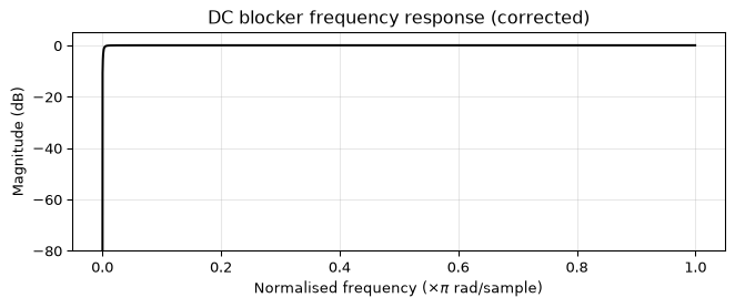

Zero: [1.]  (|z| = 1.000)
Pole: [0.995]  (|p| = 0.995)

Challenge (continued)

Exercise 16: System identification from step response data (Challenge)

A system is driven by a unit step \(u[n]\) and its output is measured. The step response \(s[n]\) settles to a final value of \(2.0\) and the first few samples are:

\(n\)	0	1	2	3	4	5
\(s[n]\)	0.60	1.02	1.314	1.520	1.664	1.765

(*approaching steady state \(s[\infty] = 2.0\))

Assume the system is first-order: \(H(z) = \frac{K}{1 - a\,z^{-1}}\).

The DC gain of \(H(z)\) equals \(s[\infty]\). Use the final value theorem to find \(K\) in terms of \(a\).
The step response of a first-order IIR satisfies \(s[n] = s[\infty]\bigl(1 - a^{n+1}\bigr)\) for \(n \geq 0\), assuming \(s[-1] = 0\). Use two consecutive samples to estimate \(a\).
Determine \(K\) and write the full transfer function. Verify by simulating and comparing to the data.

Solution

The DC gain is \(H(e^{j0}) = H(z)|_{z=1} = \frac{K}{1-a}\). Setting this equal to \(s[\infty] = 2.0\): \[K = 2(1 - a)\]
From consecutive samples: \(s[n] = 2(1 - a^{n+1})\), so \(a^{n+1} = 1 - s[n]/2\).

Using \(n = 0\): \(a = 1 - s[0]/2 = 1 - 0.30 = 0.70\).

Verify with \(n = 1\): \(s[1] = 2(1 - 0.7^2) = 2(1 - 0.49) = 2 \times 0.51 = 1.02\), which matches the table.

With the least-squares estimate of \(a\), \(K = 2(1-a)\).

import numpy as np
from scipy.signal import lfilter
from scipy.optimize import curve_fit

s_data = np.array([0.60, 1.02, 1.314, 1.520, 1.664, 1.765])
n_data = np.arange(len(s_data))
s_inf = 2.0

# Least-squares fit: s[n] = s_inf * (1 - a^{n+1})
def step_model(n, a):
    return s_inf * (1 - a**(n + 1))

popt, _ = curve_fit(step_model, n_data, s_data, p0=[0.7], bounds=(0, 1))
a_est = popt[0]
K_est = s_inf * (1 - a_est)

print(f"Estimated pole:  a = {a_est:.4f}")
print(f"Estimated gain:  K = {K_est:.4f}")
print(f"Transfer function: H(z) = {K_est:.4f} / (1 - {a_est:.4f} z^-1)")

# Simulate step response
step = np.ones(20)
h_sim = lfilter([K_est], [1, -a_est], step)

print("\nn | s_data | s_simulated")
for i in range(6):
    print(f"{i} | {s_data[i]:.3f}  | {h_sim[i]:.4f}")

print(f"\nFinal value (simulated): {h_sim[-1]:.4f}")

Estimated pole:  a = 0.7000
Estimated gain:  K = 0.6001
Transfer function: H(z) = 0.6001 / (1 - 0.7000 z^-1)

n | s_data | s_simulated
0 | 0.600  | 0.6001
1 | 1.020  | 1.0201
2 | 1.314  | 1.3141
3 | 1.520  | 1.5199
4 | 1.664  | 1.6640
5 | 1.765  | 1.7648

Final value (simulated): 1.9984

Exercise 17: Design a two-zero comb filter and analyse its trade-offs (Challenge)

A comb filter places \(M\) equally spaced zeros around the unit circle to null \(M\) harmonics simultaneously. The simplest form is:

\[H(z) = 1 - z^{-M}\]

For \(M = 4\), find all zeros of \(H(z)\) and mark their frequencies in normalised units (\(\times\pi\) rad/sample).
The comb filter’s impulse response has only two non-zero samples. What is the computational cost relative to a direct notch filter?
A classmate proposes adding a pole at \(z = r\) for each zero at \(z = e^{j2\pi k/M}\) to sharpen the nulls:

\[H_r(z) = \frac{1 - z^{-M}}{1 - r^M z^{-M}}\]

For \(M = 4\) and \(r = 0.9\), plot the magnitude response and compare the null width at \(\omega = \pi/2\) for \(r = 0\) (pure FIR) and \(r = 0.9\). Which would you choose for removing \(50\,\text{Hz}\) mains hum and its harmonics from a \(200\,\text{Hz}\)-sampled signal, and why?

Solution

Zeros where \(z^4 = 1\): \(z_k = e^{j2\pi k/4}\) for \(k = 0,1,2,3\), i.e. \(z \in \{1, j, -1, -j\}\). Normalised frequencies: \(0\), \(0.5\pi\), \(\pi\), \(1.5\pi\) rad/sample, equivalently \(\omega/\pi \in \{0, 0.5, 1, 1.5\}\), covering DC (0), \(f_s/4\) (0.5π), Nyquist (π), and \(-f_s/4\) (1.5π, aliases to the negative-frequency side of 0.5π).
The impulse response is \(h = [1, 0, 0, 0, -1]\), with two non-zero taps regardless of \(M\). Cost: 0 multiplies and 1 subtract per sample (just \(y[n] = x[n] - x[n-M]\)). A conventional notch filter targeting each harmonic would need about \(5M\) multiply-accumulate operations for \(M\) second-order sections (5 coefficients per biquad), so the comb is dramatically cheaper.
For \(M = 4\), \(H_r(z) = (1 - z^{-4})/(1 - 0.6561\,z^{-4})\). At \(f_s = 200\,\text{Hz}\), \(M = 4\) zeros target \(0, 50, 100, 150\,\text{Hz}\). The \(r = 0.9\) version narrows each null significantly. For mains hum the IIR comb is preferable: it attenuates a narrow band around each harmonic rather than a broad one, preserving more of the signal bandwidth between harmonics. The FIR comb kills a wide swath around each null frequency.

import numpy as np
import matplotlib.pyplot as plt

M = 4
w = np.linspace(0, np.pi, 2048)
z = np.exp(1j * w)

# FIR comb: H(z) = 1 - z^{-M}
H_fir = 1 - z**(-M)

# IIR comb: H_r(z) = (1 - z^{-M}) / (1 - r^M z^{-M})
r = 0.9
H_iir = (1 - z**(-M)) / (1 - r**M * z**(-M))

fig, ax = plt.subplots(figsize=(8, 4))
ax.plot(w / np.pi, 20*np.log10(np.abs(H_fir) + 1e-12),
        'b-', linewidth=1.5, label=f'FIR comb (r=0)')
ax.plot(w / np.pi, 20*np.log10(np.abs(H_iir) + 1e-12),
        'r-', linewidth=1.5, label=f'IIR comb (r={r})')
ax.axvline(0.5, color='gray', linestyle='--', linewidth=0.8, alpha=0.7)
ax.set_xlabel('Normalised frequency ($\\times \\pi$ rad/sample)')
ax.set_ylabel('Magnitude (dB)')
ax.set_title(f'Comb filter (M={M}): FIR vs IIR')
ax.set_ylim(-80, 10)
ax.legend()
ax.grid(True, alpha=0.3)
fig.tight_layout()
plt.show()

# Measure null width at omega = pi/2 (index nearest pi/2)
idx_half = np.argmin(np.abs(w - np.pi/2))
threshold_dB = -20

# Find 3dB width around pi/2 for each filter
for label, H in [('FIR', H_fir), ('IIR', H_iir)]:
    mag_dB = 20 * np.log10(np.abs(H) + 1e-12)
    region = np.where(mag_dB < threshold_dB)[0]
    # Find contiguous region around idx_half
    near = region[np.abs(region - idx_half) < 200]
    if len(near) > 0:
        bw = (w[near[-1]] - w[near[0]]) / np.pi
        print(f"{label} comb: null width at pi/2 (below {threshold_dB} dB) ≈ {bw:.3f} π rad/sample")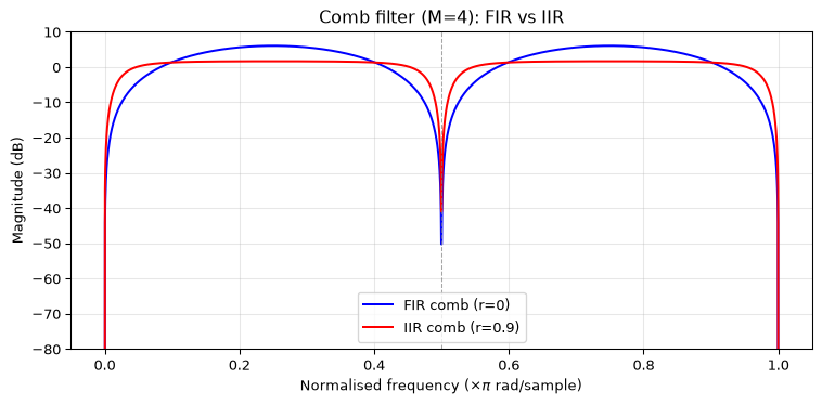

FIR comb: null width at pi/2 (below -20 dB) ≈ 0.015 π rad/sample
IIR comb: null width at pi/2 (below -20 dB) ≈ 0.005 π rad/sample

Exercise 18: Choose a pole placement for a resonator (Challenge)

You are designing a discrete-time resonator to detect a \(1\,\text{kHz}\) tone in a signal sampled at \(f_s = 8\,\text{kHz}\). The resonator transfer function is:

\[H(z) = \frac{1 - r^2}{1 - 2r\cos(\omega_0)\,z^{-1} + r^2\,z^{-2}}\]

where \(\omega_0 = 2\pi f_0 / f_s\) and the numerator \((1-r^2)\) normalises the peak gain to approximately unity at \(\omega_0\) (exact for \(r\) close to 1).

You have three candidate pole radii: \(r \in \{0.80, 0.95, 0.99\}\).

For each \(r\), compute the \(-3\,\text{dB}\) bandwidth in Hz and the approximate \(-60\,\text{dB}\) ring-down time in milliseconds.
Suppose the tone you are detecting lasts for exactly \(5\,\text{ms}\) (40 samples). Which \(r\) gives the best trade-off between frequency selectivity and fast response? Justify your answer quantitatively.
A second requirement says the filter must attenuate any \(2\,\text{kHz}\) component by at least \(20\,\text{dB}\). Check whether each candidate meets this spec.

Solution

For a second-order resonator with complex poles at \(r\,e^{\pm j\omega_0}\), the \(-3\,\text{dB}\) bandwidth is approximately \(B \approx (1-r)\,f_s/\pi\) Hz, and ring-down time to \(-60\,\text{dB}\) is \(N_{60} \approx 6.908/(-\ln r)\) samples = \(N_{60}/f_s\) seconds.
The \(5\,\text{ms}\) tone lasts 40 samples. A good rule of thumb: the filter’s ring-down time should be comparable to or shorter than the event duration. \(r = 0.99\) rings for roughly 687 samples, far longer than 40. \(r = 0.80\) settles in ~31 samples but has very broad bandwidth. \(r = 0.95\) balances selectivity (bandwidth ~127 Hz) with ring-down (~134 samples, 17 ms), usable for a 5 ms tone. In practice \(r = 0.95\) is the best compromise here.
Compute \(|H(e^{j2\pi \cdot 2000/8000})|\) for each \(r\) and compare to \(-20\,\text{dB}\) (\(= 0.1\) linear).

import numpy as np
import matplotlib.pyplot as plt
from scipy.signal import freqz

fs = 8000
f0 = 1000
omega_0 = 2 * np.pi * f0 / fs

candidates = [0.80, 0.95, 0.99]

print(f"{'r':>5} | {'BW (Hz)':>10} | {'N60 (samp)':>12} | {'T60 (ms)':>10} | {'Atten @2kHz (dB)':>18}")
print("-" * 65)

fig, ax = plt.subplots(figsize=(8, 4))
w_plot = np.linspace(0, np.pi, 2048)

for r in candidates:
    b = [1 - r**2, 0]
    a = [1, -2*r*np.cos(omega_0), r**2]

    # Bandwidth approximation
    bw_hz = (1 - r) * fs / np.pi

    # Ring-down time
    N60 = 3 * np.log(10) / (-np.log(r))
    T60_ms = N60 / fs * 1000

    # Attenuation at 2 kHz
    f2 = 2000
    omega_2 = 2 * np.pi * f2 / fs
    z2 = np.exp(1j * omega_2)
    H_at_2k = np.polyval(b, z2) / np.polyval(a, z2)
    # Need polynomial in positive powers of z: b_pos = [1-r^2, 0], a_pos = [1, -2r cos w0, r^2]
    # polyval evaluates highest power first, so this is correct for z domain
    atten_dB = 20 * np.log10(np.abs(H_at_2k))

    meets_spec = "YES" if atten_dB <= -20 else "NO "
    print(f"{r:>5.2f} | {bw_hz:>10.1f} | {N60:>12.1f} | {T60_ms:>10.1f} | {atten_dB:>12.1f} dB  {meets_spec}")

    # Frequency response for plot
    _, H = freqz(b, a, worN=w_plot)
    ax.plot(w_plot / np.pi * fs / 2, 20*np.log10(np.abs(H) + 1e-12),
            label=f'r = {r}')

ax.axhline(-20, color='gray', linestyle='--', linewidth=0.8, label='-20 dB spec')
ax.axvline(2000, color='gray', linestyle=':', linewidth=0.8)
ax.set_xlabel('Frequency (Hz)')
ax.set_ylabel('Magnitude (dB)')
ax.set_title('Resonator candidates: magnitude response')
ax.set_xlim(0, fs/2)
ax.set_ylim(-80, 10)
ax.legend()
ax.grid(True, alpha=0.3)
fig.tight_layout()
plt.show()

    r |    BW (Hz) |   N60 (samp) |   T60 (ms) |   Atten @2kHz (dB)
-----------------------------------------------------------------
 0.80 |      509.3 |         31.0 |        3.9 |        -10.4 dB  NO 
 0.95 |      127.3 |        134.7 |       16.8 |        -22.8 dB  YES
 0.99 |       25.5 |        687.3 |       85.9 |        -36.9 dB  YES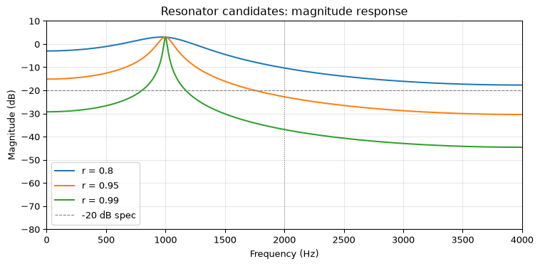

The \(-20\,\text{dB}\) specification at \(2\,\text{kHz}\) is met only by \(r = 0.95\) and \(r = 0.99\) (verify from the table above). Combined with the ring-down requirement, \(r = 0.95\) is the recommended choice: it meets the attenuation spec and has the shortest ring-down among those that do.