In Chapter 2, we described filters by their difference equations and impulse responses, all in the time domain. This works fine for FIR filters, but for IIR filters with feedback, solving the difference equation directly can be painful. A first-order IIR filter is manageable; a fourth-order one is a wall of algebra.
The z-transform sidesteps this problem. It converts sequences and difference equations into polynomials, turning convolution into multiplication and time-delays into powers of \(z^{-1}\). The result is a compact algebraic representation, the transfer function, that tells you everything about a filter’s behaviour without ever computing a single output sample.
The z-transform
The (unilateral) z-transform (Proakis and Manolakis 2007) converts a discrete-time signal \(x[n]\) into a function of the complex variable \(z\):
where \(z\) is a complex number: \(z = A\,e^{j\phi}\), with magnitude \(A\) and angle \(\phi\). Notice that \(X(z)\) is a continuous function of \(z\), even though \(x[n]\) is a discrete sequence.
The key insight: each factor of \(z^{-1}\) represents a one-sample delay. So the z-transform replaces time-shifts with algebraic multiplication, which is much easier to manipulate.
A first example
Consider a signal with four samples: \(x[0] = 0.5\), \(x[1] = 3\), \(x[2] = -0.5\), \(x[3] = 1\). Its z-transform is:
\[X(z) = 0.5 + 3\,z^{-1} - 0.5\,z^{-2} + z^{-3}\]
That’s it. Just substitute each sample value at its delay. The signal in the time domain becomes a polynomial in \(z^{-1}\).
Properties
The z-transform has three properties we’ll use constantly:
Property
Time domain
Z-domain
Linearity
\(a_1\,x_1[n] + a_2\,x_2[n]\)
\(a_1\,X_1(z) + a_2\,X_2(z)\)
Delay
\(x[n-k]\)
\(z^{-k}\,X(z)\)
Convolution
\(x_1[n] * x_2[n]\)
\(X_1(z) \cdot X_2(z)\)
The last one is the big payoff: convolution in time becomes multiplication in the z-domain. Computing a filter’s output, which requires sliding and summing in the time domain, becomes a single polynomial multiplication in the z-domain.
Transform pairs
Rather than computing the infinite sum every time, we use a short table of known pairs:
Signal
\(x[n]\)
\(X(z)\)
Kronecker delta
\(\delta[n]\)
\(1\)
Unit step
\(u[n]\)
\(\dfrac{z}{z-1}\)
Geometric sequence
\(a^n\,u[n]\)
\(\dfrac{z}{z-a}\)
Delayed signal
\(x[n-k]\)
\(z^{-k}\,X(z)\)
The unit step \(u[n]\) is defined as \(u[n] = 1\) for \(n \geq 0\) and \(u[n] = 0\) for \(n < 0\). Multiplying any signal by \(u[n]\) enforces causality: the signal is zero before \(n = 0\).
Derivation: z-transform of the geometric sequence
The geometric sequence \(a^n u[n]\) appears everywhere in IIR filter analysis. Its z-transform follows from the definition:
The last step uses the geometric series formula \(\sum_{n=0}^{\infty} r^n = \frac{1}{1-r}\), which converges when \(|r| < 1\), i.e., when \(|az^{-1}| < 1\). This convergence requirement is the region of convergence (ROC); for causal signals, it means \(|z| > |a|\).
Exercise: z-transform from the definition
Compute the z-transform of \(x[n] = -\delta[n] + 2\,\delta[n-1] - 3\,\delta[n-5]\).
Answer
Using linearity and the delay property:
\[X(z) = -1 + 2z^{-1} - 3z^{-5}\]
Each delayed delta contributes a single term at the corresponding power of \(z^{-1}\).
Transfer functions
In Chapter 2, we wrote the general difference equation:
This is the ratio of two polynomials in \(z^{-1}\). The numerator contains the feedforward coefficients \(b_i\); the denominator contains the feedback coefficients \(a_j\) (with \(a_0 = 1\) by convention).
The transfer function is also the z-transform of the impulse response:
\[H(z) = \mathcal{Z}\{h[n]\}\]
And because convolution becomes multiplication: \(Y(z) = H(z) \cdot X(z)\).
Block diagram elements in the z-domain
The three building blocks from Chapter 2 translate directly:
Operation
Time domain
Z-domain
Addition
\(y[n] = x_1[n] + x_2[n]\)
\(Y(z) = X_1(z) + X_2(z)\)
Scaling
\(y[n] = a\,x[n]\)
\(Y(z) = a\,X(z)\)
Unit delay
\(y[n] = x[n-1]\)
\(Y(z) = z^{-1}\,X(z)\)
The delay element \(T\) in a block diagram is simply replaced by \(z^{-1}\).
Note: there is no denominator polynomial (beyond the trivial \(z^2\)), confirming this is an FIR filter. For FIR filters, the filter order equals the number of delay elements.
This has one zero at \(z = 1\) and one pole at \(z = a\). The zero at \(z = 1\) forces \(H(z) = 0\) at DC (zero frequency), which is exactly what a DC blocker should do.
Exercise: Derive the transfer function
A second-order IIR filter has the difference equation:
A transfer function \(H(z)\) is a ratio of two polynomials. The roots of the numerator are the zeros (where \(H(z) = 0\)); the roots of the denominator are the poles (where \(H(z) \to \infty\)). Together with a gain constant \(K\), they completely specify the transfer function:
\[H(z) = K \frac{(z - z_1)(z - z_2) \cdots (z - z_M)}{(z - p_1)(z - p_2) \cdots (z - p_N)}\]
A pole-zero plot shows these locations on the complex z-plane: zeros are marked with \(\circ\), poles with \(\times\). The unit circle (\(|z| = 1\)) is always drawn because poles must lie inside it for stability, and it corresponds to the frequency axis (as we’ll see in Chapter 5).
Example: MA filter poles and zeros
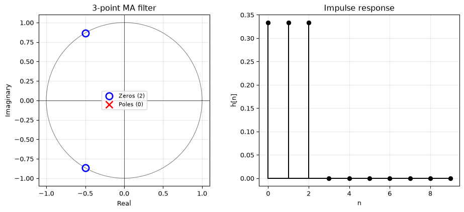
The 3-point MA filter has \(H(z) = (z^2 + z + 1) / (3z^2)\). The numerator roots are the zeros; the denominator gives poles at \(z = 0\) (a double pole at the origin).
Figure 1: Pole-zero plot of the 3-point MA filter. Two complex zeros on the unit circle, two poles at the origin.
For FIR filters, the only poles are at \(z = 0\) (trivial poles from the \(z^{-P}\) terms). FIR filters are sometimes said to have “no poles”: this is engineer’s shorthand for “no non-trivial poles.”
Example: DC blocker poles and zeros
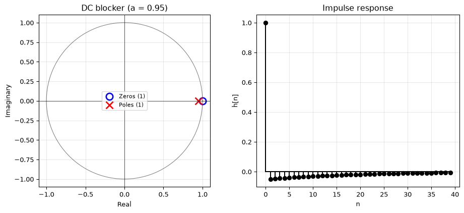
The DC blocker with \(a = 0.95\): \(H(z) = (z - 1)/(z - 0.95)\).
Figure 2: Pole-zero plot of the DC blocker (a = 0.95). The zero at z = 1 kills DC; the pole at z = 0.95 provides a sharp transition.
The pole at \(z = 0.95\) is inside the unit circle: the system is stable. The impulse response decays as \(0.95^n\), which we can verify by looking at the plot.
Example: second-order IIR filter
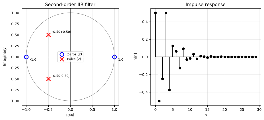
Consider a second-order filter with the difference equation \(y[n] = \frac{1}{2}x[n] - \frac{1}{2}x[n-2] - y[n-1] - \frac{1}{2}y[n-2]\), giving the transfer function \(H(z) = (z^2 - 1)/(2z^2 + 2z + 1)\).
Figure 3: Pole-zero plot of a second-order IIR filter. Complex conjugate poles inside the unit circle: the system is stable.
Notice the oscillating, decaying impulse response: this is the signature of complex conjugate poles. The oscillation frequency is related to the angle of the poles; the decay rate is related to their distance from the unit circle.
Complex conjugate poles
For filters with real coefficients, complex poles always come in conjugate pairs: if \(p = r\,e^{j\theta}\) is a pole, so is \(p^* = r\,e^{-j\theta}\). The same holds for zeros. This is why the upper and lower halves of the z-plane are mirror images.
Python: computing poles and zeros
SciPy’s tf2zpk converts transfer function coefficients to zeros, poles, and gain:
# DC blocker exampleb = [1, -1]a = [1, -0.95]zeros, poles, gain = tf2zpk(b, a)print(f"Zeros: {zeros}")print(f"Poles: {poles}")print(f"Gain: {gain}")
Zeros: [1.]
Poles: [0.95]
Gain:  1.0
From the z-domain back to time
The inverse z-transform recovers the time-domain signal:
\[h[n] = \mathcal{Z}^{-1}\{H(z)\}\]
For the filters in this chapter, we can use the transform pairs table directly without formal inversion methods.
FIR: direct readoff
The MA filter transfer function \(H(z) = \frac{1}{3}(1 + z^{-1} + z^{-2})\) inverts immediately using the delta/delay pairs:
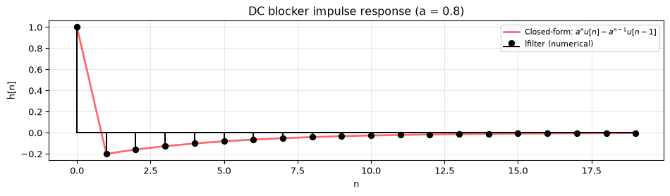
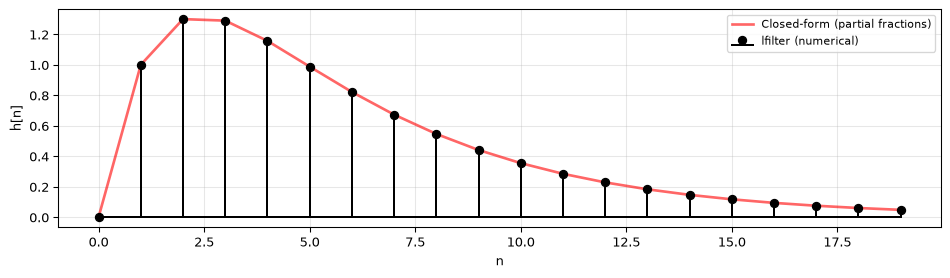
Figure 4: IIR impulse response: computed from the difference equation (dots) vs the closed-form expression (line).
The two approaches give identical results: the z-transform is a faithful representation.
Partial fraction decomposition
For higher-order transfer functions, you can’t just read off the inverse from the table. Partial fraction decomposition(Mitra 2006) breaks \(H(z)\) into a sum of simple terms, each of which has a known inverse.
The method: given \(H(z)\) with distinct poles at \(p_1, p_2, \ldots\), divide by \(z\) first, then decompose:
A system has the transfer function \(H(z) = \frac{3z}{z - 0.5}\). What is its impulse response \(h[n]\)?
Answer
From the table, \(\frac{z}{z-a} \leftrightarrow a^n u[n]\). So:
\[h[n] = 3 \cdot (0.5)^n\,u[n]\]
The impulse response starts at \(h[0] = 3\) and decays by half each sample.
Stability
A filter is only useful if it’s BIBO stable: bounded input always produces bounded output. From Chapter 2, the condition is that the impulse response must be absolutely summable:
\[\sum_{n=-\infty}^{\infty} |h[n]| < \infty\]
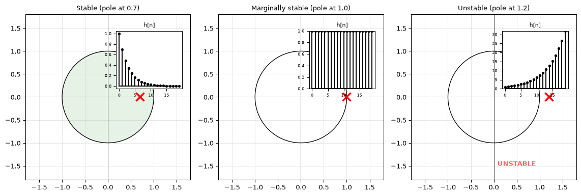
The z-transform gives us a simple graphical test (Oppenheim and Schafer 2010): a causal LTI system is BIBO stable if and only if all poles lie strictly inside the unit circle (\(|p_i| < 1\) for all \(i\)).
This makes intuitive sense. Each pole at \(z = a\) contributes a term \(a^n\) to the impulse response. If \(|a| < 1\), the term decays; if \(|a| > 1\), it grows without bound.
Figure 6: Stability regions in the z-plane. Poles inside the unit circle → stable; outside → unstable; on the circle → marginally stable.
Marginal stability
When a pole lies exactly on the unit circle (\(|a| = 1\)), the system is marginally stable: the impulse response neither decays nor grows. A pole at \(z = 1\) produces a constant (integrator); a pole at \(z = -1\) produces an alternating sequence. Marginally stable systems are useful in theory (oscillators, integrators) but fragile in practice: any rounding error can push the pole outside the circle.
Factor the denominator: \(z^2 - 0.5z - 0.5 = (z - 1)(z + 0.5)\).
The poles are at \(z = 1\) and \(z = -0.5\).
Since one pole is on the unit circle (\(|z| = 1\)), the system is marginally stable, not BIBO stable in the strict sense. The pole at \(z = 1\) means the filter has an integrator-like mode that can cause the output to drift unboundedly.
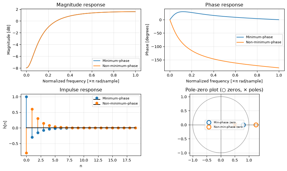
A causal, stable system is minimum-phase if all its zeros also lie inside the unit circle (\(|z_i| < 1\) for all \(i\)). This is a stronger condition than stability alone (which only requires poles inside the circle).
Why does this matter? Given a magnitude response \(|H(e^{j\omega T})|\), there are many different systems that share the same magnitude. They differ only in their phase. Among all these systems, the minimum-phase one has:
The least group delay: the output arrives as early as possible.
A causal, stable inverse: you can undo the filter by inverting \(H(z)\). Since all zeros are inside the unit circle, \(1/H(z)\) has all its poles inside the unit circle too.
Minimum energy delay: the impulse response concentrates its energy as early as possible.
Systems with zeros outside the unit circle are called non-minimum-phase. They have the same magnitude response but more phase lag. You can always factor a non-minimum-phase system into a minimum-phase part times an all-pass part (which has unit magnitude everywhere but adds phase).
from scipy.signal import freqz, group_delay# Minimum-phase: zero at z = 0.8b_min = [1, -0.8]a = [1, -0.5] # same pole for both# Non-minimum-phase: zero at z = 1/0.8 = 1.25 (reflected outside unit circle)# Scale to match DC gain: (1 - 0.8) = 0.2, (1 - 1.25) = -0.25 → multiply by -0.2/0.25 = -0.8b_nonmin = np.array([1, -1.25]) * (-0.8)fig, axes = plt.subplots(2, 2, figsize=(10, 6))# Magnitude response (should be identical up to a constant)for b, label, color in [(b_min, 'Minimum-phase', 'C0'), (b_nonmin, 'Non-minimum-phase', 'C1')]: w, H = freqz(b, a, worN=1024) axes[0, 0].plot(w/np.pi, 20*np.log10(np.abs(H)), color=color, linewidth=1.5, label=label) axes[0, 1].plot(w/np.pi, np.unwrap(np.angle(H)) *180/np.pi, color=color, linewidth=1.5, label=label)axes[0, 0].set_ylabel('Magnitude [dB]')axes[0, 0].set_title('Magnitude response')axes[0, 0].legend(fontsize=8)axes[0, 0].grid(True, alpha=0.3)axes[0, 1].set_ylabel('Phase [degrees]')axes[0, 1].set_title('Phase response')axes[0, 1].legend(fontsize=8)axes[0, 1].grid(True, alpha=0.3)# Impulse responsen = np.arange(20)delta = np.zeros(20); delta[0] =1for b, label, color in [(b_min, 'Minimum-phase', 'C0'), (b_nonmin, 'Non-minimum-phase', 'C1')]: h = lfilter(b, a, delta) axes[1, 0].stem(n, h, linefmt=color+'-', markerfmt=color+'o', basefmt='k-', label=label)axes[1, 0].set_xlabel('n')axes[1, 0].set_ylabel('h[n]')axes[1, 0].set_title('Impulse response')axes[1, 0].legend(fontsize=8)axes[1, 0].grid(True, alpha=0.3)# Pole-zero plottheta = np.linspace(0, 2*np.pi, 200)axes[1, 1].plot(np.cos(theta), np.sin(theta), 'k-', linewidth=0.8, alpha=0.5)for b, label, color in [(b_min, 'Min-phase', 'C0'), (b_nonmin, 'Non-min-phase', 'C1')]: zeros, poles, _ = tf2zpk(b, a) axes[1, 1].plot(zeros.real, zeros.imag, 'o', color=color, markersize=10, markerfacecolor='none', markeredgewidth=2, label=f'{label} zero') axes[1, 1].plot(poles.real, poles.imag, 'x', color=color, markersize=10, markeredgewidth=2)axes[1, 1].axhline(0, color='k', linewidth=0.5)axes[1, 1].axvline(0, color='k', linewidth=0.5)axes[1, 1].set_aspect('equal')axes[1, 1].set_title('Pole-zero plot (○ zeros, × poles)')axes[1, 1].legend(fontsize=7)axes[1, 1].grid(True, alpha=0.3)for ax in axes[1, :]: ax.set_xlabel(ax.get_xlabel() or'')axes[0, 0].set_xlabel('Normalized frequency [×π rad/sample]')axes[0, 1].set_xlabel('Normalized frequency [×π rad/sample]')fig.tight_layout()plt.show()
Figure 7: Minimum-phase vs non-minimum-phase systems with the same magnitude response. The minimum-phase system has less phase lag and concentrates energy earlier.
When does minimum-phase matter?
In filter design, minimum-phase is often the default: scipy.signal.butter, cheby1, etc. produce minimum-phase IIR filters. In signal processing applications like deconvolution or channel equalization, knowing that a system is minimum-phase guarantees that a stable inverse exists. Linear-phase FIR filters are not minimum-phase (their zeros come in reciprocal pairs on the unit circle), but they have other desirable properties, see Chapter 6.
Exploring pole-zero behavior
The z-plane is most powerful as a design tool when you develop intuition for how moving poles and zeros changes the filter. This section builds that intuition through exploration.
Pole radius and impulse response decay
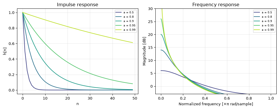
A single real pole at \(z = a\) produces an impulse response \(h[n] = a^n\,u[n]\). As the pole moves closer to the unit circle, the response decays more slowly: the filter “rings” longer and has a narrower bandwidth:
fig, axes = plt.subplots(1, 2, figsize=(10, 4))n = np.arange(50)pole_values = [0.5, 0.8, 0.9, 0.95, 0.99]colors = plt.cm.viridis(np.linspace(0.2, 0.9, len(pole_values)))for a, c inzip(pole_values, colors): h = a ** n axes[0].plot(n, h, color=c, linewidth=1.5, label=f'a = {a}')# Frequency response: H(z) = z/(z-a) w, H = freqz([1], [1, -a], worN=1024) axes[1].plot(w/np.pi, 20*np.log10(np.abs(H)), color=c, linewidth=1.5, label=f'a = {a}')axes[0].set_xlabel('n')axes[0].set_ylabel('h[n]')axes[0].set_title('Impulse response')axes[0].legend(fontsize=7)axes[0].grid(True, alpha=0.3)axes[1].set_xlabel('Normalized frequency [×π rad/sample]')axes[1].set_ylabel('Magnitude [dB]')axes[1].set_title('Frequency response')axes[1].set_ylim(-3, 30)axes[1].legend(fontsize=7)axes[1].grid(True, alpha=0.3)fig.tight_layout()plt.show()
Figure 8: Effect of pole radius on impulse response. Closer to the unit circle = slower decay = narrower bandwidth.
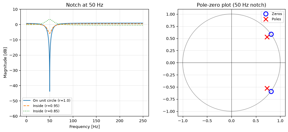
Zero placement and notch filters
Placing a zero on the unit circle at angle \(\theta\) creates a perfect null at the corresponding frequency. This is the principle behind notch filters, used to remove power-line interference (50/60 Hz), for example.
Moving the zero slightly inside the unit circle turns the perfect null into a dip. The closer the zero is to the unit circle, the deeper the notch.
fig, axes = plt.subplots(1, 2, figsize=(10, 4.5))# Notch at 50 Hz, fs = 500 Hz → ω₀ = 2π·50/500 = 0.2π rad/samplefs =500f_notch =50w0 =2* np.pi * f_notch / fs# Zeros at different radiifor r_z, ls, label in [(1.0, '-', 'On unit circle (r=1.0)'), (0.95, '--', 'Inside (r=0.95)'), (0.85, ':', 'Inside (r=0.85)')]:# Complex conjugate zero pair at angle ±ω₀ z1 = r_z * np.exp(1j* w0) z2 = r_z * np.exp(-1j* w0) b = np.real(np.poly([z1, z2]))# Add poles near the zeros for a narrow notch (not a broadband cut) p1 =0.9* np.exp(1j* w0) p2 =0.9* np.exp(-1j* w0) a = np.real(np.poly([p1, p2])) w, H = freqz(b, a, worN=2048, fs=fs) axes[0].plot(w, 20*np.log10(np.maximum(np.abs(H), 1e-10)), linestyle=ls, linewidth=1.5, label=label)axes[0].set_xlabel('Frequency [Hz]')axes[0].set_ylabel('Magnitude [dB]')axes[0].set_ylim(-60, 10)axes[0].set_title(f'Notch at {f_notch} Hz')axes[0].legend(fontsize=8)axes[0].grid(True, alpha=0.3)# Pole-zero plot for the on-unit-circle casez1 = np.exp(1j* w0)z2 = np.exp(-1j* w0)p1 =0.9* np.exp(1j* w0)p2 =0.9* np.exp(-1j* w0)theta = np.linspace(0, 2*np.pi, 200)axes[1].plot(np.cos(theta), np.sin(theta), 'k-', linewidth=0.8, alpha=0.5)axes[1].plot([z1.real, z2.real], [z1.imag, z2.imag], 'bo', markersize=10, markerfacecolor='none', markeredgewidth=2, label='Zeros')axes[1].plot([p1.real, p2.real], [p1.imag, p2.imag], 'rx', markersize=10, markeredgewidth=2, label='Poles')axes[1].axhline(0, color='k', linewidth=0.5)axes[1].axvline(0, color='k', linewidth=0.5)axes[1].set_aspect('equal')axes[1].set_title('Pole-zero plot (50 Hz notch)')axes[1].legend(fontsize=8)axes[1].grid(True, alpha=0.3)fig.tight_layout()plt.show()
Figure 9: Notch filter by zero placement. A zero on the unit circle creates a perfect null; moving it inside reduces the notch depth.
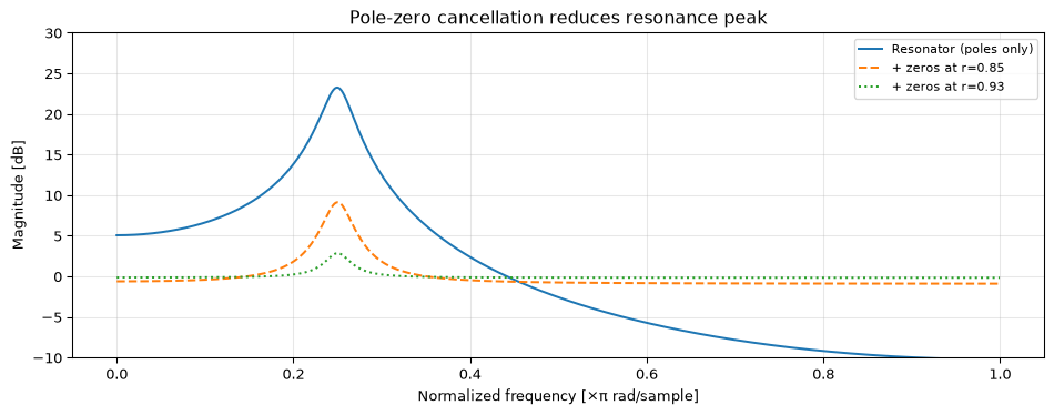
Pole-zero cancellation
When a pole and a zero are close together, they cancel each other’s effect on the frequency response. This is useful for understanding why some filter designs contain near-cancelling pairs, and why removing them barely changes the response.
fig, ax = plt.subplots(figsize=(10, 4))# Resonator: poles at r·e^{±jω₀}r =0.95w0 = np.pi /4# Without cancellation: just the resonatora_res = np.real(np.poly([r*np.exp(1j*w0), r*np.exp(-1j*w0)]))w, H1 = freqz([1], a_res, worN=2048)ax.plot(w/np.pi, 20*np.log10(np.abs(H1)), 'C0-', linewidth=1.5, label='Resonator (poles only)')# With partial cancellation: add zeros at r_z·e^{±jω₀} with r_z < rfor r_z, color, ls in [(0.85, 'C1', '--'), (0.93, 'C2', ':')]: b_cancel = np.real(np.poly([r_z*np.exp(1j*w0), r_z*np.exp(-1j*w0)])) w, H2 = freqz(b_cancel, a_res, worN=2048) ax.plot(w/np.pi, 20*np.log10(np.abs(H2)), color=color, linestyle=ls, linewidth=1.5, label=f'+ zeros at r={r_z}')ax.set_xlabel('Normalized frequency [×π rad/sample]')ax.set_ylabel('Magnitude [dB]')ax.set_ylim(-10, 30)ax.set_title('Pole-zero cancellation reduces resonance peak')ax.legend(fontsize=8)ax.grid(True, alpha=0.3)fig.tight_layout()plt.show()
Figure 10: Pole-zero cancellation: adding a zero near a pole flattens the resonance peak.
Design by pole-zero placement
These examples illustrate a powerful approach: instead of computing filter coefficients from design algorithms, you can place poles and zeros directly on the z-plane. This works well for low-order, intuitive shaping: notch filters, resonators, and simple equalisers, especially in audio and embedded systems. It does not scale to sharp, high-order frequency-selective filters (steep transition bands, tight ripple specifications), where placing dozens of poles by hand is impractical and the algorithmic methods in Chapter 6 are the right tool.
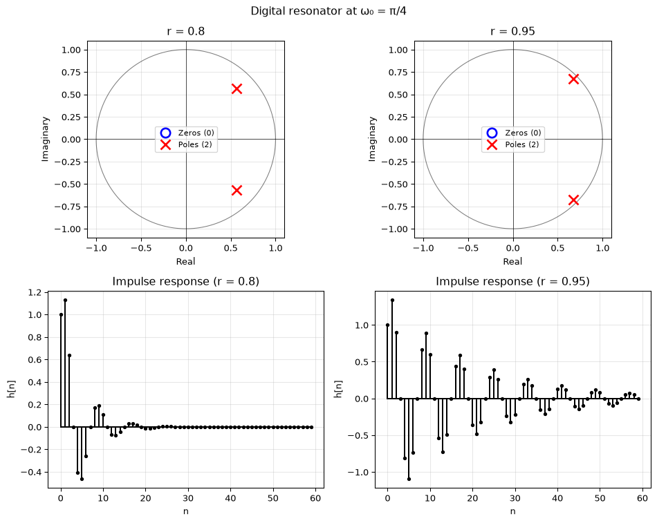
Putting it all together
Let’s trace a complete example from difference equation to pole-zero analysis. Consider a resonator, a filter that amplifies a narrow frequency band:
where \(r\) controls the resonance sharpness and \(\omega_0\) is the resonant frequency.
fig, axes = plt.subplots(2, 2, figsize=(10, 8))omega_0 = np.pi /4# resonant at π/4 radians/samplefor i, r inenumerate([0.8, 0.95]):# Transfer function coefficients b = [1] a = [1, -2*r*np.cos(omega_0), r**2]# Pole-zero plot ax_pz = axes[0, i] plot_pzmap(b, a, title=f'r = {r}', ax=ax_pz)# Impulse response ax_ir = axes[1, i] n = np.arange(60) delta = np.zeros(60) delta[0] =1 h = lfilter(b, a, delta) ax_ir.stem(n, h, linefmt='k-', markerfmt='k.', basefmt='k-') ax_ir.set_xlabel('n') ax_ir.set_ylabel('h[n]') ax_ir.set_title(f'Impulse response (r = {r})') ax_ir.grid(True, alpha=0.3)fig.suptitle(f'Digital resonator at ω₀ = π/4', fontsize=12)fig.tight_layout()plt.show()
Figure 11: A digital resonator: transfer function, pole-zero plot, and impulse response. Closer poles to the unit circle produce sharper resonance and longer ringing.
When the poles are closer to the unit circle (\(r = 0.95\)), the impulse response rings longer and the resonance is sharper. If \(r \geq 1\), the poles cross the unit circle and the system becomes unstable: the ringing grows instead of decaying. This is the z-plane telling you directly about the filter’s behaviour.
Summary
Concept
Key result
Z-transform
\(X(z) = \sum_{n=0}^{\infty} x[n]\,z^{-n}\)
Delay property
\(x[n-k] \leftrightarrow z^{-k}\,X(z)\)
Convolution → multiplication
\(y = x * h \leftrightarrow Y(z) = X(z)\,H(z)\)
Transfer function
\(H(z) = Y(z)/X(z) = \mathcal{Z}\{h[n]\}\)
Poles and zeros
Roots of denominator and numerator of \(H(z)\)
BIBO stability
All poles inside the unit circle: \(|p_i| < 1\)
The z-transform converts time-domain difference equations into algebraic transfer functions. Poles and zeros on the z-plane give immediate visual insight into stability and filter behaviour. In the next chapter, we evaluate \(H(z)\) on the unit circle to obtain the frequency response: The frequency domain.
Further reading
Oppenheim & Schafer, Discrete-Time Signal Processing (2010), Ch. 3: The z-transform
Mitra, Digital Signal Processing (2006), Ch. 5.4–5.6: Partial fractions, inverse z-transform
References
Mitra, Sanjit K. 2006. Digital Signal Processing: A Computer-Based Approach. 3rd ed. McGraw-Hill.
Oppenheim, Alan V., and Ronald W. Schafer. 2010. Discrete-Time Signal Processing. 3rd ed. Pearson.
Proakis, John G., and Dimitris G. Manolakis. 2007. Digital Signal Processing: Principles, Algorithms, and Applications. 4th ed. Pearson.
Source Code
---title: "The Z-Domain"subtitle: "Transfer functions, poles, zeros, and stability"---```{python}#| echo: falseimport numpy as npimport matplotlib.pyplot as pltfrom scipy.signal import lfilter, tf2zpk, freqz```In [Chapter 2](02-discrete-time.qmd), we described filters by their difference equations and impulse responses, all in the time domain. This works fine for FIR filters, but for IIR filters with feedback, solving the difference equation directly can be painful. A first-order IIR filter is manageable; a fourth-order one is a wall of algebra.The **z-transform** sidesteps this problem. It converts sequences and difference equations into polynomials, turning convolution into multiplication and time-delays into powers of $z^{-1}$. The result is a compact algebraic representation, the **transfer function**, that tells you everything about a filter's behaviour without ever computing a single output sample.---## The z-transformThe (unilateral) z-transform [@proakis2007digital] converts a discrete-time signal $x[n]$ into a function of the complex variable $z$:$$X(z) = \sum_{n=0}^{\infty} x[n]\, z^{-n} = x[0] + x[1]\,z^{-1} + x[2]\,z^{-2} + \cdots$$where $z$ is a complex number: $z = A\,e^{j\phi}$, with magnitude $A$ and angle $\phi$. Notice that $X(z)$ is a continuous function of $z$, even though $x[n]$ is a discrete sequence.The key insight: **each factor of $z^{-1}$ represents a one-sample delay**. So the z-transform replaces time-shifts with algebraic multiplication, which is much easier to manipulate.### A first exampleConsider a signal with four samples: $x[0] = 0.5$, $x[1] = 3$, $x[2] = -0.5$, $x[3] = 1$. Its z-transform is:$$X(z) = 0.5 + 3\,z^{-1} - 0.5\,z^{-2} + z^{-3}$$That's it. Just substitute each sample value at its delay. The signal in the time domain becomes a polynomial in $z^{-1}$.### PropertiesThe z-transform has three properties we'll use constantly:| Property | Time domain | Z-domain ||----------|------------|----------|| Linearity | $a_1\,x_1[n] + a_2\,x_2[n]$ | $a_1\,X_1(z) + a_2\,X_2(z)$ || Delay | $x[n-k]$ | $z^{-k}\,X(z)$ || Convolution | $x_1[n] * x_2[n]$ | $X_1(z) \cdot X_2(z)$ |The last one is the big payoff: **convolution in time becomes multiplication in the z-domain**. Computing a filter's output, which requires sliding and summing in the time domain, becomes a single polynomial multiplication in the z-domain.### Transform pairsRather than computing the infinite sum every time, we use a short table of known pairs:| Signal | $x[n]$ | $X(z)$ ||--------|---------|--------|| Kronecker delta | $\delta[n]$ | $1$ || Unit step | $u[n]$ | $\dfrac{z}{z-1}$ || Geometric sequence | $a^n\,u[n]$ | $\dfrac{z}{z-a}$ || Delayed signal | $x[n-k]$ | $z^{-k}\,X(z)$ |The unit step $u[n]$ is defined as $u[n] = 1$ for $n \geq 0$ and $u[n] = 0$ for $n < 0$. Multiplying any signal by $u[n]$ enforces causality: the signal is zero before $n = 0$.::: {.callout-tip collapse="true"}## Derivation: z-transform of the geometric sequenceThe geometric sequence $a^n u[n]$ appears everywhere in IIR filter analysis. Its z-transform follows from the definition:$$\mathcal{Z}\{a^n u[n]\} = \sum_{n=0}^{\infty} a^n z^{-n} = \sum_{n=0}^{\infty} (az^{-1})^n = \frac{1}{1 - az^{-1}} = \frac{z}{z-a}$$The last step uses the geometric series formula $\sum_{n=0}^{\infty} r^n = \frac{1}{1-r}$, which converges when $|r| < 1$, i.e., when $|az^{-1}| < 1$. This convergence requirement is the **region of convergence** (ROC); for causal signals, it means $|z| > |a|$.:::::: {.callout-tip collapse="true" title="Exercise: z-transform from the definition"}Compute the z-transform of $x[n] = -\delta[n] + 2\,\delta[n-1] - 3\,\delta[n-5]$.::: {.callout-note collapse="true" title="Answer"}Using linearity and the delay property:$$X(z) = -1 + 2z^{-1} - 3z^{-5}$$Each delayed delta contributes a single term at the corresponding power of $z^{-1}$.::::::---## Transfer functionsIn [Chapter 2](02-discrete-time.qmd), we wrote the general difference equation:$$y[n] = \sum_{i=0}^{P} b_i\,x[n-i] - \sum_{j=1}^{Q} a_j\,y[n-j]$$Taking the z-transform of both sides (using the linearity and delay properties) and rearranging gives the **transfer function**:$$H(z) = \frac{Y(z)}{X(z)} = \frac{b_0 + b_1\,z^{-1} + \cdots + b_P\,z^{-P}}{1 + a_1\,z^{-1} + \cdots + a_Q\,z^{-Q}}$$This is the ratio of two polynomials in $z^{-1}$. The numerator contains the feedforward coefficients $b_i$; the denominator contains the feedback coefficients $a_j$ (with $a_0 = 1$ by convention).The transfer function is also the z-transform of the impulse response:$$H(z) = \mathcal{Z}\{h[n]\}$$And because convolution becomes multiplication: $Y(z) = H(z) \cdot X(z)$.### Block diagram elements in the z-domainThe three building blocks from Chapter 2 translate directly:| Operation | Time domain | Z-domain ||-----------|------------|----------|| Addition | $y[n] = x_1[n] + x_2[n]$ | $Y(z) = X_1(z) + X_2(z)$ || Scaling | $y[n] = a\,x[n]$ | $Y(z) = a\,X(z)$ || Unit delay | $y[n] = x[n-1]$ | $Y(z) = z^{-1}\,X(z)$ |The delay element $T$ in a block diagram is simply replaced by $z^{-1}$.### Example: 3-point moving averageThe MA filter from Chapter 2:$$y[n] = \tfrac{1}{3}\bigl(x[n] + x[n-1] + x[n-2]\bigr)$$Taking the z-transform:$$Y(z) = \tfrac{1}{3}\bigl(X(z) + z^{-1}X(z) + z^{-2}X(z)\bigr) = \frac{X(z)}{3}\bigl(1 + z^{-1} + z^{-2}\bigr)$$So the transfer function is:$$H(z) = \frac{Y(z)}{X(z)} = \frac{1 + z^{-1} + z^{-2}}{3} = \frac{z^2 + z + 1}{3z^2}$$Note: there is no denominator polynomial (beyond the trivial $z^2$), confirming this is an FIR filter. For FIR filters, the filter order equals the number of delay elements.### Example: DC blocker (first-order IIR)The DC-blocking high-pass filter from Chapter 2:$$y[n] = x[n] - x[n-1] + a\,y[n-1]$$Taking the z-transform:$$Y(z) = X(z) - z^{-1}X(z) + a\,z^{-1}Y(z)$$Collecting terms:$$Y(z)\bigl(1 - a\,z^{-1}\bigr) = X(z)\bigl(1 - z^{-1}\bigr)$$$$H(z) = \frac{1 - z^{-1}}{1 - a\,z^{-1}} = \frac{z - 1}{z - a}$$This has one zero at $z = 1$ and one pole at $z = a$. The zero at $z = 1$ forces $H(z) = 0$ at DC (zero frequency), which is exactly what a DC blocker should do.::: {.callout-tip collapse="true" title="Exercise: Derive the transfer function"}A second-order IIR filter has the difference equation:$$y[n] = x[n] + b\,x[n-1] + a\,y[n-1] + c\,y[n-2]$$Derive $H(z)$.::: {.callout-note collapse="true" title="Answer"}Taking the z-transform:$$Y(z) = X(z) + b\,z^{-1}X(z) + a\,z^{-1}Y(z) + c\,z^{-2}Y(z)$$$$Y(z)\bigl(1 - a\,z^{-1} - c\,z^{-2}\bigr) = X(z)\bigl(1 + b\,z^{-1}\bigr)$$$$H(z) = \frac{1 + b\,z^{-1}}{1 - a\,z^{-1} - c\,z^{-2}}$$::::::---## The z-planeA transfer function $H(z)$ is a ratio of two polynomials. The roots of the numerator are the **zeros** (where $H(z) = 0$); the roots of the denominator are the **poles** (where $H(z) \to \infty$). Together with a gain constant $K$, they completely specify the transfer function:$$H(z) = K \frac{(z - z_1)(z - z_2) \cdots (z - z_M)}{(z - p_1)(z - p_2) \cdots (z - p_N)}$$A **pole-zero plot** shows these locations on the complex z-plane: zeros are marked with $\circ$, poles with $\times$. The **unit circle** ($|z| = 1$) is always drawn because poles must lie inside it for stability, and it corresponds to the frequency axis (as we'll see in [Chapter 5](05-frequency-domain.qmd)).```{python}#| label: pz-helper#| echo: falsedef plot_pzmap(b, a, title='', ax=None):"""Plot pole-zero map with unit circle. Accepts scipy-convention (b, a) arrays."""if ax isNone: fig, ax = plt.subplots(figsize=(5, 5))# Unit circle theta = np.linspace(0, 2* np.pi, 200) ax.plot(np.cos(theta), np.sin(theta), 'k-', linewidth=0.8, alpha=0.5)# Compute poles and zeros using scipy convention zeros, poles, _ = tf2zpk(b, a)# Plot ax.plot(zeros.real, zeros.imag, 'bo', markersize=10, markerfacecolor='none', markeredgewidth=2, label=f'Zeros ({len(zeros)})') ax.plot(poles.real, poles.imag, 'rx', markersize=10, markeredgewidth=2, label=f'Poles ({len(poles)})') ax.axhline(0, color='k', linewidth=0.5) ax.axvline(0, color='k', linewidth=0.5) ax.set_xlabel('Real') ax.set_ylabel('Imaginary') ax.set_title(title) ax.set_aspect('equal') ax.legend(fontsize=8) ax.grid(True, alpha=0.3)return ax```### Example: MA filter poles and zerosThe 3-point MA filter has $H(z) = (z^2 + z + 1) / (3z^2)$. The numerator roots are the zeros; the denominator gives poles at $z = 0$ (a double pole at the origin).```{python}#| label: fig-pz-ma#| fig-cap: "Pole-zero plot of the 3-point MA filter. Two complex zeros on the unit circle, two poles at the origin."b_ma = [1/3, 1/3, 1/3] # feedforward coefficientsa_ma = [1] # no feedback (FIR)fig, (ax1, ax2) = plt.subplots(1, 2, figsize=(10, 4.5))plot_pzmap(b_ma, a_ma, title='3-point MA filter', ax=ax1)# Show the impulse response alongsiden = np.arange(10)h = lfilter(b_ma, a_ma, np.eye(1, 10).flatten())ax2.stem(n, h, linefmt='k-', markerfmt='ko', basefmt='k-')ax2.set_xlabel('n')ax2.set_ylabel('h[n]')ax2.set_title('Impulse response')ax2.grid(True, alpha=0.3)fig.tight_layout()plt.show()```For FIR filters, the only poles are at $z = 0$ (trivial poles from the $z^{-P}$ terms). FIR filters are sometimes said to have "no poles": this is engineer's shorthand for "no non-trivial poles."### Example: DC blocker poles and zerosThe DC blocker with $a = 0.95$: $H(z) = (z - 1)/(z - 0.95)$.```{python}#| label: fig-pz-dc#| fig-cap: "Pole-zero plot of the DC blocker (a = 0.95). The zero at z = 1 kills DC; the pole at z = 0.95 provides a sharp transition."b_dc = [1, -1] # numerator: z - 1a_dc = [1, -0.95] # denominator: z - 0.95fig, (ax1, ax2) = plt.subplots(1, 2, figsize=(10, 4.5))plot_pzmap(b_dc, a_dc, title='DC blocker (a = 0.95)', ax=ax1)# Show impulse responsen = np.arange(40)delta = np.zeros(40)delta[0] =1h = lfilter([1, -1], [1, -0.95], delta)ax2.stem(n, h, linefmt='k-', markerfmt='ko', basefmt='k-')ax2.set_xlabel('n')ax2.set_ylabel('h[n]')ax2.set_title('Impulse response')ax2.grid(True, alpha=0.3)fig.tight_layout()plt.show()```The pole at $z = 0.95$ is inside the unit circle: the system is stable. The impulse response decays as $0.95^n$, which we can verify by looking at the plot.### Example: second-order IIR filterConsider a second-order filter with the difference equation $y[n] = \frac{1}{2}x[n] - \frac{1}{2}x[n-2] - y[n-1] - \frac{1}{2}y[n-2]$, giving the transfer function $H(z) = (z^2 - 1)/(2z^2 + 2z + 1)$.```{python}#| label: fig-pz-iir2#| fig-cap: "Pole-zero plot of a second-order IIR filter. Complex conjugate poles inside the unit circle: the system is stable."b_iir2 = [1, 0, -1] # numerator: 1 - z^{-2}a_iir2 = [2, 2, 1] # denominator: 2 + 2z^{-1} + z^{-2}fig, (ax1, ax2) = plt.subplots(1, 2, figsize=(10, 4.5))ax = plot_pzmap(b_iir2, a_iir2, title='Second-order IIR filter', ax=ax1)# Annotate pole and zero locationszeros, poles, _ = tf2zpk(b_iir2, a_iir2)for z in zeros: ax.annotate(f'{z.real:.1f}{z.imag:+.1f}j'if z.imag !=0elsef'{z.real:.1f}', (z.real, z.imag), textcoords='offset points', xytext=(10, -10), fontsize=8)for p in poles: ax.annotate(f'{p.real:.2f}{p.imag:+.2f}j', (p.real, p.imag), textcoords='offset points', xytext=(10, 5), fontsize=8)# Impulse responsen = np.arange(30)delta = np.zeros(30)delta[0] =1h = lfilter(b_iir2, a_iir2, delta)ax2.stem(n, h, linefmt='k-', markerfmt='ko', basefmt='k-')ax2.set_xlabel('n')ax2.set_ylabel('h[n]')ax2.set_title('Impulse response')ax2.grid(True, alpha=0.3)fig.tight_layout()plt.show()```Notice the oscillating, decaying impulse response: this is the signature of complex conjugate poles. The oscillation frequency is related to the angle of the poles; the decay rate is related to their distance from the unit circle.::: {.callout-note}## Complex conjugate polesFor filters with real coefficients, complex poles always come in conjugate pairs: if $p = r\,e^{j\theta}$ is a pole, so is $p^* = r\,e^{-j\theta}$. The same holds for zeros. This is why the upper and lower halves of the z-plane are mirror images.:::### Python: computing poles and zerosSciPy's `tf2zpk` converts transfer function coefficients to zeros, poles, and gain:```{python}# DC blocker exampleb = [1, -1]a = [1, -0.95]zeros, poles, gain = tf2zpk(b, a)print(f"Zeros: {zeros}")print(f"Poles: {poles}")print(f"Gain: {gain}")```---## From the z-domain back to timeThe inverse z-transform recovers the time-domain signal:$$h[n] = \mathcal{Z}^{-1}\{H(z)\}$$For the filters in this chapter, we can use the transform pairs table directly without formal inversion methods.### FIR: direct readoffThe MA filter transfer function $H(z) = \frac{1}{3}(1 + z^{-1} + z^{-2})$ inverts immediately using the delta/delay pairs:$$h[n] = \tfrac{1}{3}\delta[n] + \tfrac{1}{3}\delta[n-1] + \tfrac{1}{3}\delta[n-2]$$This is just the impulse response we already know from Chapter 2: the filter coefficients themselves.### IIR: using the tableThe DC blocker $H(z) = \frac{z - 1}{z - a}$ requires a bit more work. Split it into recognisable pieces:$$H(z) = \frac{z}{z-a} - \frac{1}{z-a} = \frac{z}{z-a} - z^{-1}\frac{z}{z-a}$$Using the geometric sequence pair ($\frac{z}{z-a} \leftrightarrow a^n u[n]$) and the delay property:$$h[n] = a^n\,u[n] - a^{n-1}\,u[n-1]$$Let's verify this with Python:```{python}#| label: fig-inverse-z#| fig-cap: "IIR impulse response: computed from the difference equation (dots) vs the closed-form expression (line)."a_val =0.8n = np.arange(20)# Closed-form from inverse z-transformh_formula = a_val**n - np.where(n >=1, a_val**(n-1), 0)# Numerical: apply the filter to a deltadelta = np.zeros(20)delta[0] =1h_filter = lfilter([1, -1], [1, -a_val], delta)fig, ax = plt.subplots(figsize=(10, 3))ax.plot(n, h_formula, 'r-', linewidth=2, alpha=0.6, label='Closed-form: $a^n u[n] - a^{n-1} u[n-1]$')ax.stem(n, h_filter, linefmt='k-', markerfmt='ko', basefmt='k-', label='lfilter (numerical)')ax.set_xlabel('n')ax.set_ylabel('h[n]')ax.set_title(f'DC blocker impulse response (a = {a_val})')ax.legend(fontsize=8)ax.grid(True, alpha=0.3)fig.tight_layout()plt.show()```The two approaches give identical results: the z-transform is a faithful representation.### Partial fraction decompositionFor higher-order transfer functions, you can't just read off the inverse from the table. **Partial fraction decomposition** [@mitra2006digital] breaks $H(z)$ into a sum of simple terms, each of which has a known inverse.The method: given $H(z)$ with distinct poles at $p_1, p_2, \ldots$, divide by $z$ first, then decompose:$$\frac{H(z)}{z} = \frac{A_1}{z - p_1} + \frac{A_2}{z - p_2} + \cdots$$Multiply both sides by $z$ again, and each term $\frac{A_i\,z}{z - p_i}$ inverts to $A_i\,p_i^n\,u[n]$ using the geometric sequence pair.**Worked example.** Consider a second-order system:$$H(z) = \frac{z}{(z - 0.5)(z - 0.8)}$$Divide by $z$: $\frac{H(z)}{z} = \frac{1}{(z - 0.5)(z - 0.8)}$. Using cover-up:$$A_1 = \frac{1}{z - 0.8}\bigg|_{z=0.5} = \frac{1}{-0.3} = -\frac{10}{3}, \qquad A_2 = \frac{1}{z - 0.5}\bigg|_{z=0.8} = \frac{1}{0.3} = \frac{10}{3}$$So $H(z) = \frac{-10/3 \cdot z}{z - 0.5} + \frac{10/3 \cdot z}{z - 0.8}$, giving:$$h[n] = \frac{10}{3}\bigl(0.8^n - 0.5^n\bigr)\,u[n]$$SciPy can verify this with `residuez`:```{python}#| label: fig-partial-fraction#| fig-cap: "Partial fraction decomposition verified: closed-form vs numerical impulse response."from scipy.signal import residuez# H(z) = z / [(z-0.5)(z-0.8)] = z^{-1} / [(1-0.5z^{-1})(1-0.8z^{-1})]# In scipy convention: b = [0, 1], a = conv([1,-0.5],[1,-0.8])b = [0, 1]a = np.convolve([1, -0.5], [1, -0.8])r, p, k = residuez(b, a)print(f"Residues: {r}")print(f"Poles: {p}")print(f"Direct: {k}")# Closed-formn = np.arange(20)h_formula = (10/3) * (0.8**n -0.5**n)# Numericaldelta = np.zeros(20); delta[0] =1h_numerical = lfilter(b, a, delta)fig, ax = plt.subplots(figsize=(10, 3))ax.plot(n, h_formula, 'r-', linewidth=2, alpha=0.6, label='Closed-form (partial fractions)')ax.stem(n, h_numerical, linefmt='k-', markerfmt='ko', basefmt='k-', label='lfilter (numerical)')ax.set_xlabel('n')ax.set_ylabel('h[n]')ax.legend(fontsize=8)ax.grid(True, alpha=0.3)fig.tight_layout()plt.show()```::: {.callout-tip collapse="true" title="Exercise: Inverse z-transform"}A system has the transfer function $H(z) = \frac{3z}{z - 0.5}$. What is its impulse response $h[n]$?::: {.callout-note collapse="true" title="Answer"}From the table, $\frac{z}{z-a} \leftrightarrow a^n u[n]$. So:$$h[n] = 3 \cdot (0.5)^n\,u[n]$$The impulse response starts at $h[0] = 3$ and decays by half each sample.::::::---## StabilityA filter is only useful if it's **BIBO stable**: bounded input always produces bounded output. From Chapter 2, the condition is that the impulse response must be absolutely summable:$$\sum_{n=-\infty}^{\infty} |h[n]| < \infty$$The z-transform gives us a simple graphical test [@oppenheim2010discrete]: **a causal LTI system is BIBO stable if and only if all poles lie strictly inside the unit circle** ($|p_i| < 1$ for all $i$).This makes intuitive sense. Each pole at $z = a$ contributes a term $a^n$ to the impulse response. If $|a| < 1$, the term decays; if $|a| > 1$, it grows without bound.```{python}#| label: fig-stability-regions#| fig-cap: "Stability regions in the z-plane. Poles inside the unit circle → stable; outside → unstable; on the circle → marginally stable."fig, axes = plt.subplots(1, 3, figsize=(12, 4))theta = np.linspace(0, 2* np.pi, 200)cases = [ (0.7, 'Stable (pole at 0.7)', True), (1.0, 'Marginally stable (pole at 1.0)', None), (1.2, 'Unstable (pole at 1.2)', False),]for ax, (pole, title, stable) inzip(axes, cases):# Unit circle ax.plot(np.cos(theta), np.sin(theta), 'k-', linewidth=1)# Shade regionsif stable isTrue: circle = plt.Circle((0, 0), 1, color='green', alpha=0.1) ax.add_patch(circle)elif stable isFalse: ax.text(0.5, -1.5, 'UNSTABLE', color='red', fontsize=10, fontweight='bold', ha='center', alpha=0.6)# Pole ax.plot(pole, 0, 'rx', markersize=12, markeredgewidth=2.5)# Impulse response inset n = np.arange(20) h = pole ** n# Small inset axes inset = ax.inset_axes([0.55, 0.55, 0.4, 0.35]) inset.stem(n, h, linefmt='k-', markerfmt='k.', basefmt='k-') inset.set_title('h[n]', fontsize=8) inset.tick_params(labelsize=6)ifnot stable: inset.set_ylim(0, min(h.max(), 50)) ax.axhline(0, color='k', linewidth=0.5) ax.axvline(0, color='k', linewidth=0.5) ax.set_xlim(-1.8, 1.8) ax.set_ylim(-1.8, 1.8) ax.set_aspect('equal') ax.set_title(title, fontsize=10) ax.grid(True, alpha=0.3)fig.tight_layout()plt.show()```::: {.callout-note}## Marginal stabilityWhen a pole lies exactly on the unit circle ($|a| = 1$), the system is **marginally stable**: the impulse response neither decays nor grows. A pole at $z = 1$ produces a constant (integrator); a pole at $z = -1$ produces an alternating sequence. Marginally stable systems are useful in theory (oscillators, integrators) but fragile in practice: any rounding error can push the pole outside the circle.:::### Checking stability in Python```{python}examples = {'Stable IIR': ([1, -1], [1, -0.95]),'Second-order': ([1, 0, -1], [2, 2, 1]),'Unstable': ([1], [1, -1.05]),}for name, (b, a) in examples.items(): _, poles, _ = tf2zpk(b, a) max_pole = np.max(np.abs(poles)) stable ="stable"if max_pole <1else"UNSTABLE"if max_pole >1else"marginal"print(f"{name:20s} poles: {poles} |p|_max = {max_pole:.3f} → {stable}")```::: {.callout-tip collapse="true" title="Exercise: Stability from the transfer function"}A filter has the transfer function:$$H(z) = \frac{z + 1}{z^2 - 0.5z - 0.5}$$Is it stable? Find the poles and check.::: {.callout-note collapse="true" title="Answer"}Factor the denominator: $z^2 - 0.5z - 0.5 = (z - 1)(z + 0.5)$.The poles are at $z = 1$ and $z = -0.5$.Since one pole is on the unit circle ($|z| = 1$), the system is **marginally stable**, not BIBO stable in the strict sense. The pole at $z = 1$ means the filter has an integrator-like mode that can cause the output to drift unboundedly.```{python}z, p, k = tf2zpk([1, 1], [1, -0.5, -0.5])print(f"Poles: {p}")print(f"Magnitudes: {np.abs(p)}")```::::::---## Minimum-phase systemsA causal, stable system is **minimum-phase** if all its zeros also lie inside the unit circle ($|z_i| < 1$ for all $i$). This is a stronger condition than stability alone (which only requires poles inside the circle).Why does this matter? Given a magnitude response $|H(e^{j\omega T})|$, there are many different systems that share the same magnitude. They differ only in their phase. Among all these systems, the minimum-phase one has:- **The least group delay**: the output arrives as early as possible.- **A causal, stable inverse**: you can undo the filter by inverting $H(z)$. Since all zeros are inside the unit circle, $1/H(z)$ has all its poles inside the unit circle too.- **Minimum energy delay**: the impulse response concentrates its energy as early as possible.Systems with zeros outside the unit circle are called **non-minimum-phase**. They have the same magnitude response but more phase lag. You can always factor a non-minimum-phase system into a minimum-phase part times an **all-pass** part (which has unit magnitude everywhere but adds phase).```{python}#| label: fig-minimum-phase#| fig-cap: "Minimum-phase vs non-minimum-phase systems with the same magnitude response. The minimum-phase system has less phase lag and concentrates energy earlier."from scipy.signal import freqz, group_delay# Minimum-phase: zero at z = 0.8b_min = [1, -0.8]a = [1, -0.5] # same pole for both# Non-minimum-phase: zero at z = 1/0.8 = 1.25 (reflected outside unit circle)# Scale to match DC gain: (1 - 0.8) = 0.2, (1 - 1.25) = -0.25 → multiply by -0.2/0.25 = -0.8b_nonmin = np.array([1, -1.25]) * (-0.8)fig, axes = plt.subplots(2, 2, figsize=(10, 6))# Magnitude response (should be identical up to a constant)for b, label, color in [(b_min, 'Minimum-phase', 'C0'), (b_nonmin, 'Non-minimum-phase', 'C1')]: w, H = freqz(b, a, worN=1024) axes[0, 0].plot(w/np.pi, 20*np.log10(np.abs(H)), color=color, linewidth=1.5, label=label) axes[0, 1].plot(w/np.pi, np.unwrap(np.angle(H)) *180/np.pi, color=color, linewidth=1.5, label=label)axes[0, 0].set_ylabel('Magnitude [dB]')axes[0, 0].set_title('Magnitude response')axes[0, 0].legend(fontsize=8)axes[0, 0].grid(True, alpha=0.3)axes[0, 1].set_ylabel('Phase [degrees]')axes[0, 1].set_title('Phase response')axes[0, 1].legend(fontsize=8)axes[0, 1].grid(True, alpha=0.3)# Impulse responsen = np.arange(20)delta = np.zeros(20); delta[0] =1for b, label, color in [(b_min, 'Minimum-phase', 'C0'), (b_nonmin, 'Non-minimum-phase', 'C1')]: h = lfilter(b, a, delta) axes[1, 0].stem(n, h, linefmt=color+'-', markerfmt=color+'o', basefmt='k-', label=label)axes[1, 0].set_xlabel('n')axes[1, 0].set_ylabel('h[n]')axes[1, 0].set_title('Impulse response')axes[1, 0].legend(fontsize=8)axes[1, 0].grid(True, alpha=0.3)# Pole-zero plottheta = np.linspace(0, 2*np.pi, 200)axes[1, 1].plot(np.cos(theta), np.sin(theta), 'k-', linewidth=0.8, alpha=0.5)for b, label, color in [(b_min, 'Min-phase', 'C0'), (b_nonmin, 'Non-min-phase', 'C1')]: zeros, poles, _ = tf2zpk(b, a) axes[1, 1].plot(zeros.real, zeros.imag, 'o', color=color, markersize=10, markerfacecolor='none', markeredgewidth=2, label=f'{label} zero') axes[1, 1].plot(poles.real, poles.imag, 'x', color=color, markersize=10, markeredgewidth=2)axes[1, 1].axhline(0, color='k', linewidth=0.5)axes[1, 1].axvline(0, color='k', linewidth=0.5)axes[1, 1].set_aspect('equal')axes[1, 1].set_title('Pole-zero plot (○ zeros, × poles)')axes[1, 1].legend(fontsize=7)axes[1, 1].grid(True, alpha=0.3)for ax in axes[1, :]: ax.set_xlabel(ax.get_xlabel() or'')axes[0, 0].set_xlabel('Normalized frequency [×π rad/sample]')axes[0, 1].set_xlabel('Normalized frequency [×π rad/sample]')fig.tight_layout()plt.show()```::: {.callout-note}## When does minimum-phase matter?In filter design, minimum-phase is often the default: `scipy.signal.butter`, `cheby1`, etc. produce minimum-phase IIR filters. In signal processing applications like deconvolution or channel equalization, knowing that a system is minimum-phase guarantees that a stable inverse exists. Linear-phase FIR filters are *not* minimum-phase (their zeros come in reciprocal pairs on the unit circle), but they have other desirable properties, see [Chapter 6](06-filter-design.qmd).:::---## Exploring pole-zero behaviorThe z-plane is most powerful as a design tool when you develop intuition for how moving poles and zeros changes the filter. This section builds that intuition through exploration.### Pole radius and impulse response decayA single real pole at $z = a$ produces an impulse response $h[n] = a^n\,u[n]$. As the pole moves closer to the unit circle, the response decays more slowly: the filter "rings" longer and has a narrower bandwidth:```{python}#| label: fig-pole-radius#| fig-cap: "Effect of pole radius on impulse response. Closer to the unit circle = slower decay = narrower bandwidth."fig, axes = plt.subplots(1, 2, figsize=(10, 4))n = np.arange(50)pole_values = [0.5, 0.8, 0.9, 0.95, 0.99]colors = plt.cm.viridis(np.linspace(0.2, 0.9, len(pole_values)))for a, c inzip(pole_values, colors): h = a ** n axes[0].plot(n, h, color=c, linewidth=1.5, label=f'a = {a}')# Frequency response: H(z) = z/(z-a) w, H = freqz([1], [1, -a], worN=1024) axes[1].plot(w/np.pi, 20*np.log10(np.abs(H)), color=c, linewidth=1.5, label=f'a = {a}')axes[0].set_xlabel('n')axes[0].set_ylabel('h[n]')axes[0].set_title('Impulse response')axes[0].legend(fontsize=7)axes[0].grid(True, alpha=0.3)axes[1].set_xlabel('Normalized frequency [×π rad/sample]')axes[1].set_ylabel('Magnitude [dB]')axes[1].set_title('Frequency response')axes[1].set_ylim(-3, 30)axes[1].legend(fontsize=7)axes[1].grid(True, alpha=0.3)fig.tight_layout()plt.show()```### Zero placement and notch filtersPlacing a zero on the unit circle at angle $\theta$ creates a perfect null at the corresponding frequency. This is the principle behind **notch filters**, used to remove power-line interference (50/60 Hz), for example.Moving the zero slightly inside the unit circle turns the perfect null into a dip. The closer the zero is to the unit circle, the deeper the notch.```{python}#| label: fig-notch-zeros#| fig-cap: "Notch filter by zero placement. A zero on the unit circle creates a perfect null; moving it inside reduces the notch depth."fig, axes = plt.subplots(1, 2, figsize=(10, 4.5))# Notch at 50 Hz, fs = 500 Hz → ω₀ = 2π·50/500 = 0.2π rad/samplefs =500f_notch =50w0 =2* np.pi * f_notch / fs# Zeros at different radiifor r_z, ls, label in [(1.0, '-', 'On unit circle (r=1.0)'), (0.95, '--', 'Inside (r=0.95)'), (0.85, ':', 'Inside (r=0.85)')]:# Complex conjugate zero pair at angle ±ω₀ z1 = r_z * np.exp(1j* w0) z2 = r_z * np.exp(-1j* w0) b = np.real(np.poly([z1, z2]))# Add poles near the zeros for a narrow notch (not a broadband cut) p1 =0.9* np.exp(1j* w0) p2 =0.9* np.exp(-1j* w0) a = np.real(np.poly([p1, p2])) w, H = freqz(b, a, worN=2048, fs=fs) axes[0].plot(w, 20*np.log10(np.maximum(np.abs(H), 1e-10)), linestyle=ls, linewidth=1.5, label=label)axes[0].set_xlabel('Frequency [Hz]')axes[0].set_ylabel('Magnitude [dB]')axes[0].set_ylim(-60, 10)axes[0].set_title(f'Notch at {f_notch} Hz')axes[0].legend(fontsize=8)axes[0].grid(True, alpha=0.3)# Pole-zero plot for the on-unit-circle casez1 = np.exp(1j* w0)z2 = np.exp(-1j* w0)p1 =0.9* np.exp(1j* w0)p2 =0.9* np.exp(-1j* w0)theta = np.linspace(0, 2*np.pi, 200)axes[1].plot(np.cos(theta), np.sin(theta), 'k-', linewidth=0.8, alpha=0.5)axes[1].plot([z1.real, z2.real], [z1.imag, z2.imag], 'bo', markersize=10, markerfacecolor='none', markeredgewidth=2, label='Zeros')axes[1].plot([p1.real, p2.real], [p1.imag, p2.imag], 'rx', markersize=10, markeredgewidth=2, label='Poles')axes[1].axhline(0, color='k', linewidth=0.5)axes[1].axvline(0, color='k', linewidth=0.5)axes[1].set_aspect('equal')axes[1].set_title('Pole-zero plot (50 Hz notch)')axes[1].legend(fontsize=8)axes[1].grid(True, alpha=0.3)fig.tight_layout()plt.show()```### Pole-zero cancellationWhen a pole and a zero are close together, they cancel each other's effect on the frequency response. This is useful for understanding why some filter designs contain near-cancelling pairs, and why removing them barely changes the response.```{python}#| label: fig-pz-cancel#| fig-cap: "Pole-zero cancellation: adding a zero near a pole flattens the resonance peak."fig, ax = plt.subplots(figsize=(10, 4))# Resonator: poles at r·e^{±jω₀}r =0.95w0 = np.pi /4# Without cancellation: just the resonatora_res = np.real(np.poly([r*np.exp(1j*w0), r*np.exp(-1j*w0)]))w, H1 = freqz([1], a_res, worN=2048)ax.plot(w/np.pi, 20*np.log10(np.abs(H1)), 'C0-', linewidth=1.5, label='Resonator (poles only)')# With partial cancellation: add zeros at r_z·e^{±jω₀} with r_z < rfor r_z, color, ls in [(0.85, 'C1', '--'), (0.93, 'C2', ':')]: b_cancel = np.real(np.poly([r_z*np.exp(1j*w0), r_z*np.exp(-1j*w0)])) w, H2 = freqz(b_cancel, a_res, worN=2048) ax.plot(w/np.pi, 20*np.log10(np.abs(H2)), color=color, linestyle=ls, linewidth=1.5, label=f'+ zeros at r={r_z}')ax.set_xlabel('Normalized frequency [×π rad/sample]')ax.set_ylabel('Magnitude [dB]')ax.set_ylim(-10, 30)ax.set_title('Pole-zero cancellation reduces resonance peak')ax.legend(fontsize=8)ax.grid(True, alpha=0.3)fig.tight_layout()plt.show()```::: {.callout-note}## Design by pole-zero placementThese examples illustrate a powerful approach: instead of computing filter coefficients from design algorithms, you can place poles and zeros directly on the z-plane. This works well for low-order, intuitive shaping: notch filters, resonators, and simple equalisers, especially in audio and embedded systems. It does *not* scale to sharp, high-order frequency-selective filters (steep transition bands, tight ripple specifications), where placing dozens of poles by hand is impractical and the algorithmic methods in [Chapter 6](06-filter-design.qmd) are the right tool.:::---## Putting it all togetherLet's trace a complete example from difference equation to pole-zero analysis. Consider a **resonator**, a filter that amplifies a narrow frequency band:$$y[n] = x[n] + 2r\cos(\omega_0)\,y[n-1] - r^2\,y[n-2]$$where $r$ controls the resonance sharpness and $\omega_0$ is the resonant frequency.```{python}#| label: fig-resonator#| fig-cap: "A digital resonator: transfer function, pole-zero plot, and impulse response. Closer poles to the unit circle produce sharper resonance and longer ringing."fig, axes = plt.subplots(2, 2, figsize=(10, 8))omega_0 = np.pi /4# resonant at π/4 radians/samplefor i, r inenumerate([0.8, 0.95]):# Transfer function coefficients b = [1] a = [1, -2*r*np.cos(omega_0), r**2]# Pole-zero plot ax_pz = axes[0, i] plot_pzmap(b, a, title=f'r = {r}', ax=ax_pz)# Impulse response ax_ir = axes[1, i] n = np.arange(60) delta = np.zeros(60) delta[0] =1 h = lfilter(b, a, delta) ax_ir.stem(n, h, linefmt='k-', markerfmt='k.', basefmt='k-') ax_ir.set_xlabel('n') ax_ir.set_ylabel('h[n]') ax_ir.set_title(f'Impulse response (r = {r})') ax_ir.grid(True, alpha=0.3)fig.suptitle(f'Digital resonator at ω₀ = π/4', fontsize=12)fig.tight_layout()plt.show()```When the poles are closer to the unit circle ($r = 0.95$), the impulse response rings longer and the resonance is sharper. If $r \geq 1$, the poles cross the unit circle and the system becomes unstable: the ringing grows instead of decaying. This is the z-plane telling you directly about the filter's behaviour.---## Summary| Concept | Key result ||---------|-----------|| Z-transform | $X(z) = \sum_{n=0}^{\infty} x[n]\,z^{-n}$ || Delay property | $x[n-k] \leftrightarrow z^{-k}\,X(z)$ || Convolution → multiplication | $y = x * h \leftrightarrow Y(z) = X(z)\,H(z)$ || Transfer function | $H(z) = Y(z)/X(z) = \mathcal{Z}\{h[n]\}$ || Poles and zeros | Roots of denominator and numerator of $H(z)$ || BIBO stability | All poles inside the unit circle: $|p_i| < 1$ |The z-transform converts time-domain difference equations into algebraic transfer functions. Poles and zeros on the z-plane give immediate visual insight into stability and filter behaviour. In the next chapter, we evaluate $H(z)$ on the unit circle to obtain the **frequency response**: [The frequency domain](05-frequency-domain.qmd).::: {.callout-note title="Further reading"}- Oppenheim & Schafer, *Discrete-Time Signal Processing* (2010), Ch. 3: The z-transform- Mitra, *Digital Signal Processing* (2006), Ch. 5.4–5.6: Partial fractions, inverse z-transform:::## References::: {#refs}:::