Yes, firwin produces symmetric (linear-phase) impulse responses by default. This means all frequencies experience the same delay: no phase distortion.
The cutoff stays at 300 Hz. The Blackman window has a wider main lobe than Hamming, so the transition width increases. But its side lobes are lower (−58 dB vs −43 dB), so stopband attenuation improves.
Elliptic achieves the sharpest transition for a given order by allowing ripple in both bands.
Exercise 4: SOS vs direct form
A 10th-order Butterworth filter is designed with butter(10, 200, fs=1000).
How many biquad sections does the SOS form have?
How many delay elements does each biquad need (DF II)?
Why might the direct-form (b, a) implementation become unstable even though all poles are inside the unit circle?
Solution
\(\lceil 10/2 \rceil = 5\) sections.
2 delay elements per biquad (DF II is the canonical form with minimum delays).
The 11-element a polynomial has coefficients that must represent 10 roots with high precision. Floating-point rounding in the 64-bit coefficients can effectively shift poles outside the unit circle. With SOS, each section only has 2 poles, so coefficient errors stay small and localised.
Intermediate
Exercise 5: Design and compare FIR methods
Design FIR lowpass filters for the same specification (\(f_p = 400\) Hz, \(f_s = 600\) Hz, \(f_\text{samp} = 4000\) Hz) using:
Window method: firwin(N, cutoff, fs=fs) with a Hamming window.
Parks–McClellan: remez(N, bands, desired, fs=fs).
Use the same order \(N = 61\) for both. Plot both magnitude responses and compare the stopband attenuation.
The Parks–McClellan filter has equiripple behaviour: the stopband ripple is evenly distributed, so the worst-case attenuation is better than the window method for the same order. The window method has deeper nulls in some places but higher peaks in others.
Exercise 6: Bilinear transform by hand
A first-order analog lowpass filter has transfer function \(H_a(s) = 1 / (1 + s/\omega_c)\) with \(\omega_c = 2\pi \times 500\) rad/s.
Apply the bilinear transform \(s = \frac{2}{T}\frac{z-1}{z+1}\) with \(f_s = 4000\) Hz to derive \(H_d(z)\).
What are the digital filter coefficients \((b_0, b_1, a_0, a_1)\)?
At what digital frequency does the analog cutoff \(\omega_c\) actually appear? (Hint: apply the warping formula.)
Solution
With \(T = 1/4000\) and \(\omega_c = 2\pi \times 500 = 3141.6\) rad/s:
The warping formula gives \(\omega_d = \frac{2}{T}\arctan\frac{\omega_c T}{2} = 8000 \times \arctan(0.393) = 8000 \times 0.3745 = 2996\) rad/s, or \(f_d = 476.8\) Hz. The cutoff is slightly lower than the analog 500 Hz due to frequency warping.
Butterworth:  N = 37
Chebyshev I:  N = 13
Elliptic:     N = 7
Elliptic: it needs the fewest biquad sections, meaning fewer multiply-accumulate operations per sample and lower power consumption. The cost is ripple in both bands, which is usually acceptable for sensor data.
Challenge
Exercise 8: Notch filter for power-line interference
A biomedical signal sampled at \(f_s = 500\) Hz is contaminated by 50 Hz power-line interference.
Design a second-order IIR notch filter by placing zeros on the unit circle at \(\theta = 2\pi \times 50/500\) and poles at the same angle with radius \(R = 0.95\). Write out the transfer function \(H(z)\).
Implement the filter with lfilter and verify the frequency response.
Generate a test signal (a 10 Hz ECG-like pulse train + 50 Hz interference) and demonstrate the filter’s effect.
This produces unity gain at DC and Nyquist, with a boost or cut of \(G_\text{dB}\) at \(\omega_0\).
import numpy as npimport matplotlib.pyplot as pltfrom scipy.signal import freqz, lfilter, welchfs =44100def peaking_eq(f0, gain_dB, Q, fs):"""Audio EQ Cookbook peaking EQ biquad.""" A =10**(gain_dB /40) w0 =2* np.pi * f0 / fs alpha = np.sin(w0) / (2* Q) b = np.array([1+ alpha * A, -2* np.cos(w0), 1- alpha * A]) a = np.array([1+ alpha / A, -2* np.cos(w0), 1- alpha / A])return b / a[0], a / a[0] # normalise so a[0] = 1def high_shelf(f0, gain_dB, Q, fs):"""Audio EQ Cookbook high shelf biquad.""" A =10**(gain_dB /40) w0 =2* np.pi * f0 / fs alpha = np.sin(w0) / (2* Q) cos_w0 = np.cos(w0) sqrtA = np.sqrt(A) b = np.array([ A * ((A +1) + (A -1)*cos_w0 +2*sqrtA*alpha),-2*A * ((A -1) + (A +1)*cos_w0), A * ((A +1) + (A -1)*cos_w0 -2*sqrtA*alpha) ]) a = np.array([ (A +1) - (A -1)*cos_w0 +2*sqrtA*alpha,2* ((A -1) - (A +1)*cos_w0), (A +1) - (A -1)*cos_w0 -2*sqrtA*alpha ])return b / a[0], a / a[0]# a) Design each bandb_bass, a_bass = peaking_eq(100, +6, 1.0, fs)b_mid, a_mid = peaking_eq(1000, -4, 2.0, fs)b_treble, a_treble = high_shelf(8000, +3, 0.707, fs)# Combined frequency responsew_freq = np.linspace(0, np.pi, 4096)H_total = np.ones(len(w_freq), dtype=complex)for b, a in [(b_bass, a_bass), (b_mid, a_mid), (b_treble, a_treble)]: _, H = freqz(b, a, worN=w_freq) H_total *= Hf_hz = w_freq * fs / (2* np.pi)fig, axes = plt.subplots(2, 1, figsize=(10, 7))# b) Combined responseaxes[0].semilogx(f_hz[1:], 20*np.log10(np.maximum(np.abs(H_total[1:]), 1e-10)),'C0-', linewidth=2)axes[0].set_xlabel('Frequency [Hz]')axes[0].set_ylabel('Gain [dB]')axes[0].set_xlim(20, fs/2)axes[0].set_ylim(-10, 10)axes[0].set_title('3-band equalizer response')axes[0].grid(True, alpha=0.3, which='both')axes[0].axhline(0, color='k', linewidth=0.5)# c) Filter white noise and compare PSDrng = np.random.default_rng(42)N =5* fsx = rng.standard_normal(N)y = x.copy()for b, a in [(b_bass, a_bass), (b_mid, a_mid), (b_treble, a_treble)]: y = lfilter(b, a, y)f_x, psd_x = welch(x, fs, nperseg=4096)f_y, psd_y = welch(y, fs, nperseg=4096)axes[1].semilogx(f_x[1:], 10*np.log10(np.maximum(psd_y[1:], 1e-20)/ np.maximum(psd_x[1:], 1e-20)),'C0-', linewidth=1.5, label='Measured EQ curve')axes[1].set_xlabel('Frequency [Hz]')axes[1].set_ylabel('Gain [dB]')axes[1].set_xlim(20, fs/2)axes[1].set_ylim(-10, 10)axes[1].set_title('Measured equalizer effect (output PSD / input PSD)')axes[1].grid(True, alpha=0.3, which='both')axes[1].axhline(0, color='k', linewidth=0.5)fig.tight_layout()plt.show()
The PSD ratio confirms the designed EQ curve: +6 dB bass boost around 100 Hz, −4 dB dip near 1 kHz, and +3 dB treble lift above 8 kHz.
Exercise 10: Debug: wrong frequency normalisation (Basic)
A student wants a 4th-order Butterworth lowpass filter with a −3 dB cutoff at 200 Hz, sampled at 1000 Hz. Here is their code:
from scipy.signal import butter, sosfiltimport numpy as npfs =1000fc =200# Hzsos = butter(4, fc, btype='low', output='sos')
Run the code. What cutoff frequency does this actually produce? Why?
Fix the single error so the filter has its −3 dB point at 200 Hz.
How would the answer change if fs = 8000 Hz?
Solution
butter with no fs argument expects the cutoff as a normalised frequency in the range \([0, 1]\), where 1.0 maps to the Nyquist frequency. Passing fc = 200 is interpreted as \(200 \times f_\text{nyq}\), which is far outside the valid range. SciPy will raise a ValueError: Digital filter critical frequencies must be 0 < Wn < 1.
Supply the sampling rate so SciPy handles the normalisation:
from scipy.signal import butter, sosfilt, sosfreqzimport numpy as npimport matplotlib.pyplot as pltfs =1000fc =200sos = butter(4, fc, btype='low', fs=fs, output='sos')w, H = sosfreqz(sos, worN=2048, fs=fs)mag_dB =20* np.log10(np.maximum(np.abs(H), 1e-10))idx = np.argmin(np.abs(mag_dB - (-3)))print(f"−3 dB point: {w[idx]:.1f} Hz (target: {fc} Hz)")
−3 dB point: 200.0 Hz (target: 200 Hz)
With fs = 8000 Hz the correct call becomes butter(4, 200, btype='low', fs=8000, output='sos'). The normalised frequency changes to \(200/4000 = 0.05\), so the same physical cutoff now sits much closer to DC on the normalised scale; the filter is “sharper” relative to Nyquist but still correct in Hz.
Exercise 11: Choosing a filter family (Basic)
For each scenario below, name the most appropriate IIR filter family (Butterworth, Chebyshev I, Chebyshev II, or Elliptic) and give a one-sentence justification.
A medical-grade ECG monitor where no passband distortion is allowed but you can tolerate slight stopband ripple.
A consumer audio application where you want the sharpest possible roll-off for a given filter order and can accept ripple in both bands.
A control loop anti-aliasing filter where the passband must be as flat as possible and the stopband rejection only needs to meet a minimum spec.
A software-defined radio front-end where strict stopband rejection is needed but any passband ripple is unacceptable.
Solution
Chebyshev II: the passband is maximally flat (monotonic), and the equiripple behaviour is confined entirely to the stopband.
Elliptic: equiripple in both passband and stopband gives the steepest possible transition for a given order, so the cutoff between bands is sharpest.
Butterworth: maximally flat magnitude response in both bands; no ripple anywhere, which simplifies characterisation of the control-loop gain margin.
Chebyshev II: the stopband meets a hard equiripple floor while the passband remains ripple-free. (Elliptic achieves a sharper roll-off but sacrifices passband flatness, which is disallowed here.)
Exercise 12: Debug: lfilter vs sosfilt for high-order filters (Basic)
A student designs a 12th-order Chebyshev I lowpass filter and notices the output looks wrong: saturated or all zeros. Here is the code:
from scipy.signal import cheby1, lfilterimport numpy as npfs =1000rng = np.random.default_rng(0)x = rng.standard_normal(5000)b, a = cheby1(12, 0.5, 200, fs=fs)y = lfilter(b, a, x)print(y[:5])
What is likely causing the incorrect output?
Fix the code using the numerically stable approach.
What is the rule of thumb for when to switch from lfilter(b, a, ...) to sosfilt?
Solution
High-order filters in direct-form (b, a) representation suffer from coefficient quantisation errors. A 12th-order polynomial has 13 coefficients that must collectively represent 12 poles. Small floating-point rounding errors shift pole locations, often placing poles outside the unit circle. The filter becomes unstable and the output diverges (or underflows to zero after overflow).
Design and filter using second-order sections:
from scipy.signal import cheby1, sosfilt, lfilterimport numpy as npfs =1000rng = np.random.default_rng(0)x = rng.standard_normal(5000)# Broken: direct formb, a = cheby1(12, 0.5, 200, fs=fs)y_bad = lfilter(b, a, x)# Fixed: SOS formsos = cheby1(12, 0.5, 200, fs=fs, output='sos')y_good = sosfilt(sos, x)print(f"Direct form output — first 5 values: {y_bad[:5]}")print(f"SOS output — first 5 values: {y_good[:5]}")print(f"Direct form has NaNs or Infs: {not np.all(np.isfinite(y_bad))}")print(f"SOS output is finite: {np.all(np.isfinite(y_good))}")
Direct form output — first 5 values: [4.88494588e-07 8.44580017e-06 7.17938764e-05 4.03723456e-04
 1.70045105e-03]
SOS output        — first 5 values:  [4.88494588e-07 8.44580017e-06 7.17938764e-05 4.03723456e-04
 1.70045105e-03]
Direct form has NaNs or Infs: False
SOS output is finite:          True
The rule of thumb: use SOS whenever the filter order exceeds about 4–6. Each biquad section has only two poles, so coefficient errors remain small and localised rather than accumulating across a high-degree polynomial.
Intermediate (continued)
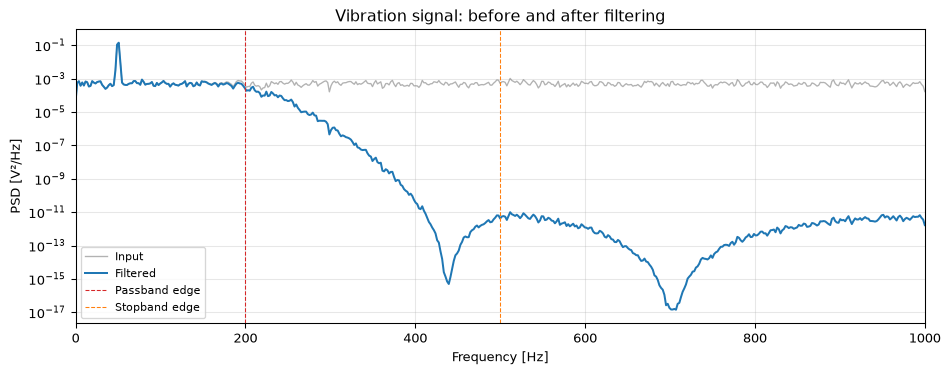
Exercise 13: Data-driven: clean a noisy vibration signal (Intermediate)
A vibration sensor on a rotating machine runs at \(f_s = 2000\) Hz. The useful content is below 200 Hz; everything above 500 Hz is broadband noise. Design and apply an appropriate filter.
Synthesise a test signal: a 50 Hz sinusoid (amplitude 1.0) plus white noise at 0 dB SNR.
Design a filter that meets: passband edge 200 Hz (≤ 1 dB ripple), stopband edge 500 Hz (≥ 40 dB attenuation). Use the minimum-order IIR family that achieves this, chosen for flat passband.
Apply the filter with zero-phase processing (sosfiltfilt) and plot the input PSD and output PSD on the same axes.
Estimate the SNR of the 50 Hz tone before and after filtering.
Solution
import numpy as npimport matplotlib.pyplot as pltfrom scipy.signal import cheb2ord, cheby2, sosfilt, sosfiltfilt, sosfreqz, welchrng = np.random.default_rng(42)fs =2000N =4* fs # 4 secondst = np.arange(N) / fssignal = np.sin(2* np.pi *50* t) # 50 Hz tone, power = 0.5noise = rng.standard_normal(N) / np.sqrt(2) # noise power = 0.5 → 0 dB SNRx = signal + noise# b) Minimum order — flat passband → Chebyshev II (flat passband, equiripple stopband)order, Wn = cheb2ord(200, 500, 1, 40, fs=fs)print(f"Chebyshev II order: {order}")sos = cheby2(order, 40, Wn, fs=fs, output='sos')# c) Zero-phase filteringy = sosfiltfilt(sos, x)# PSDf_x, Pxx = welch(x, fs, nperseg=1024)f_y, Pyy = welch(y, fs, nperseg=1024)fig, ax = plt.subplots(figsize=(10, 4))ax.semilogy(f_x, Pxx, 'C7-', linewidth=1, alpha=0.6, label='Input')ax.semilogy(f_y, Pyy, 'C0-', linewidth=1.5, label='Filtered')ax.axvline(200, color='C3', linewidth=0.8, linestyle='--', label='Passband edge')ax.axvline(500, color='C1', linewidth=0.8, linestyle='--', label='Stopband edge')ax.set_xlabel('Frequency [Hz]')ax.set_ylabel('PSD [V²/Hz]')ax.set_title('Vibration signal: before and after filtering')ax.legend(fontsize=8)ax.grid(True, alpha=0.3)ax.set_xlim(0, fs/2)fig.tight_layout()plt.show()# d) SNR estimate: signal power at 50 Hz bin vs. noise floor# Approximate SNR: ratio of peak PSD bin to median noise floor (density ratio, not integrated power)def tone_snr(signal_clean, x_noisy, fs, f_tone, nperseg=1024): f, Pxx = welch(x_noisy, fs, nperseg=nperseg) idx = np.argmin(np.abs(f - f_tone)) signal_power = Pxx[idx] noise_floor = np.median(Pxx)return10* np.log10(signal_power / noise_floor)snr_before = tone_snr(signal, x, fs, 50)snr_after = tone_snr(signal, y, fs, 50)print(f"SNR before filtering: {snr_before:.1f} dB")print(f"SNR after filtering: {snr_after:.1f} dB")
Chebyshev II order: 4
SNR before filtering: 24.6 dB
SNR after  filtering: 105.1 dB
The zero-phase filter suppresses the broadband noise above 500 Hz without introducing phase distortion; the 50 Hz tone is recovered with clearly improved SNR. Note that sosfiltfilt doubles the effective order (applies the filter twice), so a lower design order suffices for the same attenuation spec.
Exercise 14: FIR vs IIR: latency trade-off (Intermediate)
You are filtering a real-time audio stream at \(f_s = 48000\) Hz for live performance monitoring. The specification requires a lowpass filter at 4 kHz (−3 dB) with 1 dB passband ripple, stopband ≥ 60 dB above 6 kHz.
Estimate the minimum FIR order using the Harris rule of thumb \(N \approx A_s / (22 \Delta f / f_s)\) where \(\Delta f = f_\text{stop} - f_\text{pass}\) and \(A_s\) is stopband attenuation in dB. What is the one-way latency in milliseconds?
Find the minimum-order elliptic IIR filter with the same specification. What is the filter order and how many biquad sections does it need?
For a live concert system the round-trip latency budget is 10 ms total. Allowing 4 ms for the filter, can you use FIR? Can you use IIR? Justify your choice.
FIR order (Harris): ~66, one-way latency: 0.68 ms
Elliptic IIR order: 6, biquad sections: 3
IIR one-way latency: effectively 0 (causal, real-time)
The elliptic filter requires far fewer sections and introduces only one sample of computational latency (the processing delay of the algorithm), not a structural group delay.
At ~0.67 ms one-way the FIR fits within the 4 ms budget, and importantly it is linear-phase, so all frequencies in the passband arrive simultaneously. The IIR introduces frequency-dependent group delay (phase distortion) but essentially zero structural latency. For live performance monitoring the IIR is preferred because it minimises perceptible latency, and small phase differences across 0–4 kHz are generally inaudible in a monitoring context. If the task were audio recording where phase accuracy matters, the FIR (or zero-phase IIR offline) would be better.
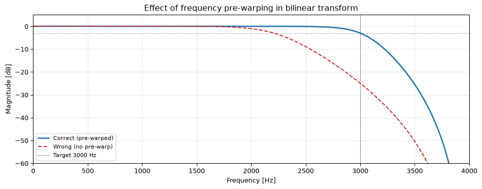
Exercise 15: Debug: forgotten frequency pre-warping (Intermediate)
A student designs a digital Butterworth lowpass filter with a cutoff at exactly 3 kHz (\(f_s = 8000\) Hz) by directly converting an analog prototype. The code below produces the wrong digital cutoff. Identify the bug and fix it.
from scipy.signal import butter, freqzimport numpy as npfs =8000fc_digital =3000# Hz — desired digital cutoff# Student converts Hz to rad/s for analog designwc_analog =2* np.pi * fc_digital # ← student's pre-warp step# Design analog prototype and bilinear transform manually via buttersos = butter(4, wc_analog, btype='low', analog=True, output='sos')# Student then expects the digital cutoff to be at 3000 Hz
Explain why the cutoff will not be at 3 kHz.
Write the correct pre-warping formula and show what wc_analog should be.
Demonstrate both designs by plotting their digital frequency responses.
Solution
The bilinear transform compresses the entire analog frequency axis \([0, \infty)\) onto the digital interval \([0, \pi)\) through the nonlinear mapping \(\omega_a = (2/T)\tan(\omega_d T/2)\). Passing the raw digital radian frequency \(2\pi f_c\) as if it were already the analog frequency ignores this warping; the resulting digital cutoff will be shifted.
import numpy as npimport matplotlib.pyplot as pltfrom scipy.signal import butter, sosfilt, sosfreqz, bilinear_zpkfs =8000T =1/ fsfc =3000# Hz — desired digital cutoff (close to Nyquist to make warping visible)# Correct pre-warped analog frequencywc_correct =2* fs * np.tan(np.pi * fc / fs)# Student's (wrong) analog frequency — used ω_d directlywc_wrong =2* np.pi * fcprint(f"Digital cutoff target: {fc} Hz")print(f"Wrong analog freq (no warp): {wc_wrong:.0f} rad/s")print(f"Correct pre-warped analog freq: {wc_correct:.0f} rad/s")print(f"Ratio (correct/wrong): {wc_correct/wc_wrong:.3f}")# Correct: scipy handles pre-warping internallysos_correct = butter(4, fc, btype='low', fs=fs, output='sos')# Wrong: design analog prototype at wrong frequency, then apply bilinear manuallyfrom scipy.signal import butter as butter_analog, zpk2sosz_w, p_w, k_w = butter_analog(4, wc_wrong, btype='low', output='zpk', analog=True)z_d, p_d, k_d = bilinear_zpk(z_w, p_w, k_w, fs)sos_wrong = zpk2sos(z_d, p_d, k_d)w, H_c = sosfreqz(sos_correct, worN=4096, fs=fs)_, H_w = sosfreqz(sos_wrong, worN=4096, fs=fs)fig, ax = plt.subplots(figsize=(10, 4))ax.plot(w, 20*np.log10(np.maximum(np.abs(H_c), 1e-10)), 'C0-', linewidth=2, label='Correct (pre-warped)')ax.plot(w, 20*np.log10(np.maximum(np.abs(H_w), 1e-10)), 'C3--', linewidth=1.5, label='Wrong (no pre-warp)')ax.axvline(fc, color='k', linewidth=0.8, linestyle=':', label=f'Target {fc} Hz')ax.axhline(-3, color='gray', linewidth=0.5, linestyle='--')ax.set_xlabel('Frequency [Hz]')ax.set_ylabel('Magnitude [dB]')ax.set_xlim(0, fs/2)ax.set_ylim(-60, 5)ax.set_title('Effect of frequency pre-warping in bilinear transform')ax.legend(fontsize=8)ax.grid(True, alpha=0.3)fig.tight_layout()plt.show()
Digital cutoff target:         3000 Hz
Wrong analog freq (no warp):   18850 rad/s
Correct pre-warped analog freq: 38627 rad/s
Ratio (correct/wrong):         2.049
The key takeaway: SciPy’s butter(N, fc, fs=fs) performs the pre-warping internally. The bug arises only if you use the analog=True path and manually pass a digital frequency. Always let SciPy handle the bilinear transform unless you have a specific reason to work in the analog domain.
Challenge (continued)
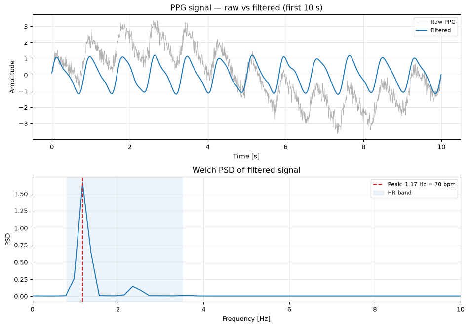
Exercise 16: Data-driven: extract heart-rate from a PPG trace (Challenge)
A photoplethysmography (PPG) sensor measures blood volume changes at \(f_s = 100\) Hz. The raw signal contains:
A strong DC baseline (offset)
A fundamental heart-rate component in the range 0.8–3.5 Hz (48–210 bpm)
Motion artefacts below 0.5 Hz
High-frequency noise above 8 Hz
Design a bandpass filter that passes 0.8–3.5 Hz and attenuates outside 0.5–8 Hz by at least 40 dB. Choose the IIR family and order using buttord or an equivalent *ord function.
Apply the filter with zero-phase processing. Synthesise a test PPG signal to validate (use a 1.2 Hz fundamental plus harmonics, a 0.1 Hz drift, and broadband noise).
Estimate the heart rate from the filtered signal by finding the dominant frequency in the 0.8–3.5 Hz band using Welch’s method. Report the result in bpm.
The dominant PSD peak falls within 0.01 Hz of the true heart-rate frequency. Key design choices: Butterworth for a smooth passband (no ripple distortion on the waveform shape), zero-phase sosfiltfilt to avoid phase shift between beats, and Welch’s method to average out noise in the PSD estimate.
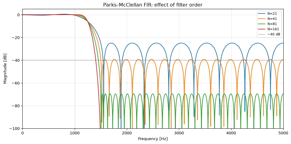
The design triangle states that for a fixed filter family and filter type, you can freely choose any two of: (1) transition width, (2) ripple/attenuation, (3) filter order, and the third is then determined.
For a Parks–McClellan FIR lowpass filter with \(f_\text{pass} = 1\) kHz, \(f_\text{samp} = 10\) kHz: use remez and freqz to sweep filter orders \(N \in \{21, 41, 81, 161\}\). For each order, measure the achieved stopband attenuation (in dB) and transition width (frequency where the magnitude first drops to −40 dB). Record both in a table.
You are handed a fixed hardware budget: the processor can execute exactly 80 multiply-accumulate operations per sample. Accounting for symmetric FIR structure (roughly halving the multiplies), what is the maximum FIR order that fits?
Under that order constraint, what stopband attenuation is achievable with a 500 Hz transition band? With a 200 Hz transition band? Comment on the design trade-off.
Solution
import numpy as npimport matplotlib.pyplot as pltfrom scipy.signal import remez, freqzfs =10000def measure_filter(N, fp, fs, plot=False):"""Design PM filter and measure attenuation and -40 dB transition width."""# Place stopband edge at fp + 500 Hz as a starting reference fst = fp +500 fst =min(fst, fs/2-10) h = remez(N, [0, fp, fst, fs/2], [1, 0], fs=fs) w, H = freqz(h, [1], worN=8192, fs=fs) mag_dB =20* np.log10(np.maximum(np.abs(H), 1e-12))# Stopband attenuation: worst case above fst sb_mask = w > fst sb_atten =-np.max(mag_dB[sb_mask]) if np.any(sb_mask) else np.nan# -40 dB transition point idx_40 = np.where(mag_dB <=-40)[0] f_40dB = w[idx_40[0]] iflen(idx_40) >0else np.nan tw_40 = f_40dB - fp ifnot np.isnan(f_40dB) else np.nanreturn h, w, mag_dB, sb_atten, tw_40fp =1000orders = [21, 41, 81, 161]print(f"{'N':>5}{'Stopband atten (dB)':>20}{'Transition to −40 dB (Hz)':>26}")print("-"*57)fig, ax = plt.subplots(figsize=(10, 5))results = []for N in orders: h, w, mag_dB, sb_atten, tw = measure_filter(N, fp, fs) results.append((N, sb_atten, tw))print(f"{N:>5}{sb_atten:>20.1f}{tw:>26.0f}") ax.plot(w, mag_dB, linewidth=1.5, label=f'N={N}')ax.axhline(-40, color='k', linewidth=0.5, linestyle='--', label='−40 dB')ax.axvline(fp, color='gray', linewidth=0.5, linestyle=':')ax.set_xlabel('Frequency [Hz]')ax.set_ylabel('Magnitude [dB]')ax.set_ylim(-100, 5)ax.set_xlim(0, fs/2)ax.set_title('Parks–McClellan FIR: effect of filter order')ax.legend(fontsize=8)ax.grid(True, alpha=0.3)fig.tight_layout()plt.show()
    N   Stopband atten (dB)   Transition to −40 dB (Hz)
---------------------------------------------------------
   21                  24.9                         545
   41                  39.3                         501
   81                  69.6                         454
  161                 127.6                         404
A length-\(N\) FIR filter with symmetric coefficients needs \(\lceil N/2 \rceil\) multiplications per output sample. For 80 MACs: \(\lceil N/2 \rceil \leq 80 \Rightarrow N \leq 159\). So the maximum order is \(N = 159\) (odd, to maintain linear phase).
Design at \(N = 159\) with the two transition bands:
Transition 500 Hz, N=159: stopband attenuation ≈ 127.3 dB
Transition 200 Hz, N=159: stopband attenuation ≈ 58.2 dB
With the 500 Hz transition band the hardware-limited filter achieves good attenuation; narrowing to a 200 Hz transition band (without increasing \(N\)) forces the equiripple algorithm to trade attenuation for transition sharpness: the stopband floor rises (worse rejection). This directly illustrates the design triangle: at fixed order, narrowing the transition band costs attenuation.
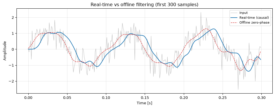
Exercise 18: Debug: zero-phase filtering on a causal real-time system (Challenge)
A student processes a streaming sensor signal in fixed-size blocks of 256 samples at \(f_s = 1000\) Hz. They copy a filter call from an offline analysis script and notice the output lags behind by roughly the expected group delay, but their manager insists the latency is unacceptable.
Here is the relevant code:
from scipy.signal import butter, sosfiltfiltimport numpy as npsos = butter(4, 50, btype='low', fs=1000, output='sos')def process_block(block, sos):return sosfiltfilt(sos, block) # ← used in real-time loop
Identify the two distinct errors that make sosfiltfilt inappropriate here.
Propose a correct real-time implementation using sosfilt with persistent state across blocks. Sketch the stateful block-processing loop.
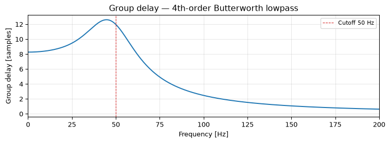
With sosfilt (causal, not zero-phase), what is the group delay of the 4th-order Butterworth filter at 20 Hz? At DC? (Use group_delay from scipy.)
Solution
Two problems:
sosfiltfilt is non-causal: it filters the block forwards and then backwards. The backward pass requires future samples that have not yet arrived in a streaming system. You cannot run sosfiltfilt on a live stream block-by-block.
No state is preserved across blocks: sosfiltfilt (and sosfilt if called naively) initialises the filter state to zero at the start of each block. Discontinuities at block boundaries produce artefacts (clicks, impulse-like transients) in the output.
Correct real-time implementation with persistent state:
The causal real-time output is shifted to the right relative to the zero-phase version; the group delay is visible as a time offset. The waveform shape is preserved; there are no block-boundary glitches because zi carries the filter memory forward.
Group delay at   0 Hz: 8.25 samples = 8.25 ms
Group delay at  20 Hz: 8.94 samples = 8.94 ms
Group delay at  50 Hz: 11.95 samples = 11.95 ms
/tmp/ipykernel_2950/4038571414.py:8: UserWarning: The filter's denominator is extremely small at frequencies [3.141], around which a singularity may be present
  w, gd = group_delay((b, a), w=4096, fs=fs)
The group delay is frequency-dependent for an IIR filter, unlike a linear-phase FIR where different frequencies experience different delays. Near DC and deep in the passband the delay is roughly constant but it rises sharply near the cutoff frequency. This is the fundamental cost of IIR phase response: phase distortion that cannot be avoided in a causal implementation.
Source Code
---title: "Exercises: Filter Design"subtitle: "Practice problems for Chapter 6"---These exercises accompany [Chapter 6: Filter Design](../basics/06-filter-design.qmd).::: {.callout-note title="Key formulas for this chapter"}| Formula | Description ||---------|-------------|| FIR group delay: $(N-1)/2$ samples | Linear-phase FIR delay || Bilinear pre-warping: $\omega_a = \frac{2}{T}\tan(\omega_d T/2)$ | Analog-to-digital frequency mapping || FIR order (Harris rule): $N \approx A_s \cdot f_s / (22 \cdot \Delta f)$ | Order estimation from specs || Always use SOS form for IIR filters of order $\geq 4$ | Numerical stability rule || `butter(N, fc, fs=fs, output='sos')` | Scipy handles pre-warping internally |:::## Basic::: {.callout-tip collapse="true" title="Exercise 1: Filter specification vocabulary"}A lowpass filter specification states: $f_p = 500$ Hz, $f_s = 700$ Hz, $\delta_p = 0.5$ dB, $A_s = 50$ dB, at $f_\text{samp} = 4000$ Hz.a) What is the transition bandwidth in Hz?b) What is the normalised transition width $\Delta f / f_\text{nyq}$?c) If you increase the stopband attenuation to 80 dB while keeping all else fixed, what happens to the required filter order?::: {.callout-note collapse="true" title="Solution"}a) Transition bandwidth = $f_s - f_p = 700 - 500 = 200$ Hz.b) $f_\text{nyq} = 2000$ Hz. Normalised width = $200/2000 = 0.1$.c) The required order increases. The design triangle tells us: with transition width and ripple fixed, demanding more attenuation forces a higher order.::::::::: {.callout-tip collapse="true" title="Exercise 2: Window method basics"}You design a 31-tap FIR lowpass filter using `firwin` with a Hamming window at $f_s = 2000$ Hz and cutoff 300 Hz.a) What is the group delay of this filter in samples? In milliseconds?b) Is the impulse response symmetric? What does that imply about the phase?c) If you switch to a Blackman window (same $N$), what changes: the cutoff frequency, the transition width, or the stopband attenuation?::: {.callout-note collapse="true" title="Solution"}a) Group delay = $(N-1)/2 = 15$ samples = $15/2000 = 7.5$ ms.b) Yes, `firwin` produces symmetric (linear-phase) impulse responses by default. This means all frequencies experience the same delay: no phase distortion.c) The cutoff stays at 300 Hz. The Blackman window has a wider main lobe than Hamming, so the transition width increases. But its side lobes are lower (−58 dB vs −43 dB), so stopband attenuation improves.::::::::: {.callout-tip collapse="true" title="Exercise 3: IIR filter families"}Match each IIR family to its characteristic:| Family | Characteristic ||--------|---------------|| Butterworth | ??? || Chebyshev I | ??? || Chebyshev II | ??? || Elliptic | ??? |Options: (A) Equiripple in both bands, (B) Maximally flat everywhere, (C) Equiripple passband + monotonic stopband, (D) Flat passband + equiripple stopband.::: {.callout-note collapse="true" title="Solution"}| Family | Characteristic ||--------|---------------|| Butterworth | **(B)** Maximally flat everywhere || Chebyshev I | **(C)** Equiripple passband + monotonic stopband || Chebyshev II | **(D)** Flat passband + equiripple stopband || Elliptic | **(A)** Equiripple in both bands |Elliptic achieves the sharpest transition for a given order by allowing ripple in both bands.::::::::: {.callout-tip collapse="true" title="Exercise 4: SOS vs direct form"}A 10th-order Butterworth filter is designed with `butter(10, 200, fs=1000)`.a) How many biquad sections does the SOS form have?b) How many delay elements does each biquad need (DF II)?c) Why might the direct-form `(b, a)` implementation become unstable even though all poles are inside the unit circle?::: {.callout-note collapse="true" title="Solution"}a) $\lceil 10/2 \rceil = 5$ sections.b) 2 delay elements per biquad (DF II is the canonical form with minimum delays).c) The 11-element `a` polynomial has coefficients that must represent 10 roots with high precision. Floating-point rounding in the 64-bit coefficients can effectively shift poles outside the unit circle. With SOS, each section only has 2 poles, so coefficient errors stay small and localised.::::::## Intermediate::: {.callout-tip collapse="true" title="Exercise 5: Design and compare FIR methods"}Design FIR lowpass filters for the same specification ($f_p = 400$ Hz, $f_s = 600$ Hz, $f_\text{samp} = 4000$ Hz) using:a) Window method: `firwin(N, cutoff, fs=fs)` with a Hamming window.b) Parks–McClellan: `remez(N, bands, desired, fs=fs)`.Use the same order $N = 61$ for both. Plot both magnitude responses and compare the stopband attenuation.::: {.callout-note collapse="true" title="Solution"}```{python}import numpy as npimport matplotlib.pyplot as pltfrom scipy.signal import firwin, remez, freqzfs =4000N =61h_win = firwin(N, 500, fs=fs, window='hamming') # cutoff at midpoint of transition bandh_pm = remez(N, [0, 400, 600, fs/2], [1, 0], fs=fs)fig, ax = plt.subplots(figsize=(10, 4))for h, label in [(h_win, 'Window (Hamming)'), (h_pm, 'Parks–McClellan')]: w, H = freqz(h, [1], worN=2048, fs=fs) ax.plot(w, 20*np.log10(np.maximum(np.abs(H), 1e-10)), linewidth=1.5, label=label)ax.set_xlabel('Frequency [Hz]')ax.set_ylabel('Magnitude [dB]')ax.set_ylim(-80, 5)ax.legend(fontsize=8)ax.grid(True, alpha=0.3)ax.set_title(f'FIR comparison (N={N})')fig.tight_layout()plt.show()```The Parks–McClellan filter has equiripple behaviour: the stopband ripple is evenly distributed, so the *worst-case* attenuation is better than the window method for the same order. The window method has deeper nulls in some places but higher peaks in others.::::::::: {.callout-tip collapse="true" title="Exercise 6: Bilinear transform by hand"}A first-order analog lowpass filter has transfer function $H_a(s) = 1 / (1 + s/\omega_c)$ with $\omega_c = 2\pi \times 500$ rad/s.a) Apply the bilinear transform $s = \frac{2}{T}\frac{z-1}{z+1}$ with $f_s = 4000$ Hz to derive $H_d(z)$.b) What are the digital filter coefficients $(b_0, b_1, a_0, a_1)$?c) At what digital frequency does the analog cutoff $\omega_c$ actually appear? (Hint: apply the warping formula.)::: {.callout-note collapse="true" title="Solution"}a) With $T = 1/4000$ and $\omega_c = 2\pi \times 500 = 3141.6$ rad/s:$$H_d(z) = \frac{1}{1 + \frac{1}{\omega_c}\frac{2}{T}\frac{z-1}{z+1}} = \frac{1 + z^{-1}}{(1 + \frac{2}{\omega_c T}) + (1 - \frac{2}{\omega_c T})z^{-1}}$$Compute $\frac{2}{\omega_c T} = \frac{2 \times 4000}{3141.6} = 2.5465$:$$H_d(z) = \frac{1 + z^{-1}}{3.5465 + (-1.5465)z^{-1}} = \frac{0.2820(1 + z^{-1})}{1 - 0.4361\,z^{-1}}$$b) $b_0 = b_1 = 0.2820$, $a_0 = 1$, $a_1 = -0.4361$.c) The warping formula gives $\omega_d = \frac{2}{T}\arctan\frac{\omega_c T}{2} = 8000 \times \arctan(0.393) = 8000 \times 0.3745 = 2996$ rad/s, or $f_d = 476.8$ Hz. The cutoff is slightly lower than the analog 500 Hz due to frequency warping.```{python}import numpy as npfrom scipy.signal import freqzfs =4000wc =2* np.pi *500T =1/fsalpha =2/ (wc * T)b0 =1/ (1+ alpha)a1 = (1- alpha) / (1+ alpha)b = [b0, b0]a = [1, a1]print(f"b = [{b[0]:.4f}, {b[1]:.4f}]")print(f"a = [1, {a[1]:.4f}]")# Verify -3 dB pointw, H = freqz(b, a, worN=2048, fs=fs)mag_dB =20* np.log10(np.abs(H))idx_3dB = np.argmin(np.abs(mag_dB - (-3)))print(f"−3 dB frequency: {w[idx_3dB]:.1f} Hz (expected ~476 Hz)")```::::::::: {.callout-tip collapse="true" title="Exercise 7: Minimum order design"}You need a lowpass filter with: $f_p = 1$ kHz, $f_s = 1.2$ kHz, $\delta_p = 1$ dB, $A_s = 60$ dB, $f_\text{samp} = 8$ kHz.a) Use `buttord`, `cheb1ord`, and `ellipord` to find the minimum order for each family.b) Design all three filters (SOS form) and plot their magnitude responses on the same axes.c) Which filter would you choose for a battery-powered embedded device? Why?::: {.callout-note collapse="true" title="Solution"}```{python}import numpy as npimport matplotlib.pyplot as pltfrom scipy.signal import buttord, cheb1ord, ellipord, butter, cheby1, ellip, sosfreqzfs =8000fp, fst =1000, 1200rp, As =1, 60Nb, Wb = buttord(fp, fst, rp, As, fs=fs)Nc, Wc = cheb1ord(fp, fst, rp, As, fs=fs)Ne, We = ellipord(fp, fst, rp, As, fs=fs)print(f"Butterworth: N = {Nb}")print(f"Chebyshev I: N = {Nc}")print(f"Elliptic: N = {Ne}")sos_b = butter(Nb, Wb, fs=fs, output='sos')sos_c = cheby1(Nc, rp, Wc, fs=fs, output='sos')sos_e = ellip(Ne, rp, As, We, fs=fs, output='sos')fig, ax = plt.subplots(figsize=(10, 4))for sos, name in [(sos_b, f'Butterworth (N={Nb})'), (sos_c, f'Chebyshev I (N={Nc})'), (sos_e, f'Elliptic (N={Ne})')]: w, H = sosfreqz(sos, worN=4096, fs=fs) ax.plot(w, 20*np.log10(np.maximum(np.abs(H), 1e-10)), linewidth=1.5, label=name)ax.axhline(-rp, color='gray', linewidth=0.5, linestyle='--')ax.axhline(-As, color='gray', linewidth=0.5, linestyle='--')ax.set_xlabel('Frequency [Hz]')ax.set_ylabel('Magnitude [dB]')ax.set_xlim(0, 3000)ax.set_ylim(-80, 5)ax.legend(fontsize=8)ax.grid(True, alpha=0.3)fig.tight_layout()plt.show()```c) **Elliptic**: it needs the fewest biquad sections, meaning fewer multiply-accumulate operations per sample and lower power consumption. The cost is ripple in both bands, which is usually acceptable for sensor data.::::::## Challenge::: {.callout-tip collapse="true" title="Exercise 8: Notch filter for power-line interference"}A biomedical signal sampled at $f_s = 500$ Hz is contaminated by 50 Hz power-line interference.a) Design a second-order IIR notch filter by placing zeros on the unit circle at $\theta = 2\pi \times 50/500$ and poles at the same angle with radius $R = 0.95$. Write out the transfer function $H(z)$.b) Implement the filter with `lfilter` and verify the frequency response.c) Generate a test signal (a 10 Hz ECG-like pulse train + 50 Hz interference) and demonstrate the filter's effect.::: {.callout-note collapse="true" title="Solution"}a) $\theta = 2\pi \times 50/500 = \pi/5$ rad.Zeros at $z = e^{\pm j\pi/5}$: numerator $(1 - e^{j\theta}z^{-1})(1 - e^{-j\theta}z^{-1}) = 1 - 2\cos\theta\,z^{-1} + z^{-2}$.Poles at $z = 0.95\,e^{\pm j\pi/5}$: denominator $1 - 2R\cos\theta\,z^{-1} + R^2 z^{-2}$.$$H(z) = \frac{1 - 2\cos(\pi/5)\,z^{-1} + z^{-2}}{1 - 1.9\cos(\pi/5)\,z^{-1} + 0.9025\,z^{-2}}$$```{python}import numpy as npimport matplotlib.pyplot as pltfrom scipy.signal import freqz, lfilterfs =500f_notch =50theta =2* np.pi * f_notch / fsR =0.95b = [1, -2*np.cos(theta), 1]a = [1, -2*R*np.cos(theta), R**2]# b) Frequency responsew, H = freqz(b, a, worN=4096, fs=fs)fig, axes = plt.subplots(1, 2, figsize=(10, 4))axes[0].plot(w, 20*np.log10(np.maximum(np.abs(H), 1e-10)), 'C0-', linewidth=1.5)axes[0].axvline(f_notch, color='C3', linewidth=0.5, linestyle='--')axes[0].set_xlabel('Frequency [Hz]')axes[0].set_ylabel('Magnitude [dB]')axes[0].set_ylim(-50, 5)axes[0].set_title('Notch filter response')axes[0].grid(True, alpha=0.3)# c) Test signalrng = np.random.default_rng(42)t = np.arange(5* fs) / fsecg_pulse = np.zeros_like(t)for beat_time in np.arange(0, 5, 0.1): # 10 Hz pulse train idx =int(beat_time * fs)if idx <len(ecg_pulse) -10: ecg_pulse[idx:idx+10] += np.hanning(10)interference =0.5* np.sin(2* np.pi *50* t)x = ecg_pulse + interference +0.05* rng.standard_normal(len(t))y = lfilter(b, a, x)t_plot =slice(0, 500) # first secondaxes[1].plot(t[t_plot], x[t_plot], 'b-', linewidth=0.5, alpha=0.5, label='Noisy')axes[1].plot(t[t_plot], y[t_plot], 'C0-', linewidth=1, label='Filtered')axes[1].set_xlabel('Time [s]')axes[1].set_ylabel('Amplitude')axes[1].set_title('50 Hz removal')axes[1].legend(fontsize=8)axes[1].grid(True, alpha=0.3)fig.tight_layout()plt.show()```::::::::: {.callout-tip collapse="true" title="Exercise 9: Audio equalizer with biquads"}Design a 3-band audio equalizer using cascaded biquad sections. The sampling rate is $f_s = 44100$ Hz.- **Bass boost**: +6 dB peaking filter centred at 100 Hz, $Q = 1$.- **Mid cut**: −4 dB peaking filter centred at 1000 Hz, $Q = 2$.- **Treble shelf**: +3 dB high-shelf above 8000 Hz.a) Use the Audio EQ Cookbook peaking EQ formula to design the biquad coefficients for the bass and mid bands.b) Cascade the three sections and plot the combined frequency response.c) Generate a white noise signal, filter it, and plot the before/after PSD to verify the equalizer curve.::: {.callout-note collapse="true" title="Solution"}The peaking EQ biquad from Robert Bristow-Johnson's Audio EQ Cookbook:$$A = 10^{G_\text{dB}/40}, \quad \alpha = \frac{\sin\omega_0}{2Q}$$$$b_0 = 1 + \alpha A, \quad b_1 = -2\cos\omega_0, \quad b_2 = 1 - \alpha A$$$$a_0 = 1 + \alpha/A, \quad a_1 = -2\cos\omega_0, \quad a_2 = 1 - \alpha/A$$This produces unity gain at DC and Nyquist, with a boost or cut of $G_\text{dB}$ at $\omega_0$.```{python}import numpy as npimport matplotlib.pyplot as pltfrom scipy.signal import freqz, lfilter, welchfs =44100def peaking_eq(f0, gain_dB, Q, fs):"""Audio EQ Cookbook peaking EQ biquad.""" A =10**(gain_dB /40) w0 =2* np.pi * f0 / fs alpha = np.sin(w0) / (2* Q) b = np.array([1+ alpha * A, -2* np.cos(w0), 1- alpha * A]) a = np.array([1+ alpha / A, -2* np.cos(w0), 1- alpha / A])return b / a[0], a / a[0] # normalise so a[0] = 1def high_shelf(f0, gain_dB, Q, fs):"""Audio EQ Cookbook high shelf biquad.""" A =10**(gain_dB /40) w0 =2* np.pi * f0 / fs alpha = np.sin(w0) / (2* Q) cos_w0 = np.cos(w0) sqrtA = np.sqrt(A) b = np.array([ A * ((A +1) + (A -1)*cos_w0 +2*sqrtA*alpha),-2*A * ((A -1) + (A +1)*cos_w0), A * ((A +1) + (A -1)*cos_w0 -2*sqrtA*alpha) ]) a = np.array([ (A +1) - (A -1)*cos_w0 +2*sqrtA*alpha,2* ((A -1) - (A +1)*cos_w0), (A +1) - (A -1)*cos_w0 -2*sqrtA*alpha ])return b / a[0], a / a[0]# a) Design each bandb_bass, a_bass = peaking_eq(100, +6, 1.0, fs)b_mid, a_mid = peaking_eq(1000, -4, 2.0, fs)b_treble, a_treble = high_shelf(8000, +3, 0.707, fs)# Combined frequency responsew_freq = np.linspace(0, np.pi, 4096)H_total = np.ones(len(w_freq), dtype=complex)for b, a in [(b_bass, a_bass), (b_mid, a_mid), (b_treble, a_treble)]: _, H = freqz(b, a, worN=w_freq) H_total *= Hf_hz = w_freq * fs / (2* np.pi)fig, axes = plt.subplots(2, 1, figsize=(10, 7))# b) Combined responseaxes[0].semilogx(f_hz[1:], 20*np.log10(np.maximum(np.abs(H_total[1:]), 1e-10)),'C0-', linewidth=2)axes[0].set_xlabel('Frequency [Hz]')axes[0].set_ylabel('Gain [dB]')axes[0].set_xlim(20, fs/2)axes[0].set_ylim(-10, 10)axes[0].set_title('3-band equalizer response')axes[0].grid(True, alpha=0.3, which='both')axes[0].axhline(0, color='k', linewidth=0.5)# c) Filter white noise and compare PSDrng = np.random.default_rng(42)N =5* fsx = rng.standard_normal(N)y = x.copy()for b, a in [(b_bass, a_bass), (b_mid, a_mid), (b_treble, a_treble)]: y = lfilter(b, a, y)f_x, psd_x = welch(x, fs, nperseg=4096)f_y, psd_y = welch(y, fs, nperseg=4096)axes[1].semilogx(f_x[1:], 10*np.log10(np.maximum(psd_y[1:], 1e-20)/ np.maximum(psd_x[1:], 1e-20)),'C0-', linewidth=1.5, label='Measured EQ curve')axes[1].set_xlabel('Frequency [Hz]')axes[1].set_ylabel('Gain [dB]')axes[1].set_xlim(20, fs/2)axes[1].set_ylim(-10, 10)axes[1].set_title('Measured equalizer effect (output PSD / input PSD)')axes[1].grid(True, alpha=0.3, which='both')axes[1].axhline(0, color='k', linewidth=0.5)fig.tight_layout()plt.show()```The PSD ratio confirms the designed EQ curve: +6 dB bass boost around 100 Hz, −4 dB dip near 1 kHz, and +3 dB treble lift above 8 kHz.::::::::: {.callout-tip collapse="true" title="Exercise 10: Debug: wrong frequency normalisation (Basic)"}A student wants a 4th-order Butterworth lowpass filter with a −3 dB cutoff at 200 Hz, sampled at 1000 Hz. Here is their code:```pythonfrom scipy.signal import butter, sosfiltimport numpy as npfs =1000fc =200# Hzsos = butter(4, fc, btype='low', output='sos')```a) Run the code. What cutoff frequency does this actually produce? Why?b) Fix the single error so the filter has its −3 dB point at 200 Hz.c) How would the answer change if `fs = 8000` Hz?::: {.callout-note collapse="true" title="Solution"}a) `butter` with no `fs` argument expects the cutoff as a *normalised* frequency in the range $[0, 1]$, where 1.0 maps to the Nyquist frequency. Passing `fc = 200` is interpreted as $200 \times f_\text{nyq}$, which is far outside the valid range. SciPy will raise a `ValueError: Digital filter critical frequencies must be 0 < Wn < 1`.b) Supply the sampling rate so SciPy handles the normalisation:```{python}from scipy.signal import butter, sosfilt, sosfreqzimport numpy as npimport matplotlib.pyplot as pltfs =1000fc =200sos = butter(4, fc, btype='low', fs=fs, output='sos')w, H = sosfreqz(sos, worN=2048, fs=fs)mag_dB =20* np.log10(np.maximum(np.abs(H), 1e-10))idx = np.argmin(np.abs(mag_dB - (-3)))print(f"−3 dB point: {w[idx]:.1f} Hz (target: {fc} Hz)")```c) With `fs = 8000` Hz the correct call becomes `butter(4, 200, btype='low', fs=8000, output='sos')`. The normalised frequency changes to $200/4000 = 0.05$, so the same physical cutoff now sits much closer to DC on the normalised scale; the filter is "sharper" relative to Nyquist but still correct in Hz.::::::::: {.callout-tip collapse="true" title="Exercise 11: Choosing a filter family (Basic)"}For each scenario below, name the most appropriate IIR filter family (Butterworth, Chebyshev I, Chebyshev II, or Elliptic) and give a one-sentence justification.a) A medical-grade ECG monitor where no passband distortion is allowed but you can tolerate slight stopband ripple.b) A consumer audio application where you want the sharpest possible roll-off for a given filter order and can accept ripple in both bands.c) A control loop anti-aliasing filter where the passband must be as flat as possible and the stopband rejection only needs to meet a minimum spec.d) A software-defined radio front-end where strict stopband rejection is needed but any passband ripple is unacceptable.::: {.callout-note collapse="true" title="Solution"}a) **Chebyshev II**: the passband is maximally flat (monotonic), and the equiripple behaviour is confined entirely to the stopband.b) **Elliptic**: equiripple in both passband and stopband gives the steepest possible transition for a given order, so the cutoff between bands is sharpest.c) **Butterworth**: maximally flat magnitude response in both bands; no ripple anywhere, which simplifies characterisation of the control-loop gain margin.d) **Chebyshev II**: the stopband meets a hard equiripple floor while the passband remains ripple-free. (Elliptic achieves a sharper roll-off but sacrifices passband flatness, which is disallowed here.)::::::::: {.callout-tip collapse="true" title="Exercise 12: Debug: lfilter vs sosfilt for high-order filters (Basic)"}A student designs a 12th-order Chebyshev I lowpass filter and notices the output looks wrong: saturated or all zeros. Here is the code:```pythonfrom scipy.signal import cheby1, lfilterimport numpy as npfs =1000rng = np.random.default_rng(0)x = rng.standard_normal(5000)b, a = cheby1(12, 0.5, 200, fs=fs)y = lfilter(b, a, x)print(y[:5])```a) What is likely causing the incorrect output?b) Fix the code using the numerically stable approach.c) What is the rule of thumb for when to switch from `lfilter(b, a, ...)` to `sosfilt`?::: {.callout-note collapse="true" title="Solution"}a) High-order filters in direct-form `(b, a)` representation suffer from coefficient quantisation errors. A 12th-order polynomial has 13 coefficients that must collectively represent 12 poles. Small floating-point rounding errors shift pole locations, often placing poles outside the unit circle. The filter becomes unstable and the output diverges (or underflows to zero after overflow).b) Design and filter using second-order sections:```{python}from scipy.signal import cheby1, sosfilt, lfilterimport numpy as npfs =1000rng = np.random.default_rng(0)x = rng.standard_normal(5000)# Broken: direct formb, a = cheby1(12, 0.5, 200, fs=fs)y_bad = lfilter(b, a, x)# Fixed: SOS formsos = cheby1(12, 0.5, 200, fs=fs, output='sos')y_good = sosfilt(sos, x)print(f"Direct form output — first 5 values: {y_bad[:5]}")print(f"SOS output — first 5 values: {y_good[:5]}")print(f"Direct form has NaNs or Infs: {not np.all(np.isfinite(y_bad))}")print(f"SOS output is finite: {np.all(np.isfinite(y_good))}")```c) The rule of thumb: **use SOS whenever the filter order exceeds about 4–6**. Each biquad section has only two poles, so coefficient errors remain small and localised rather than accumulating across a high-degree polynomial.::::::## Intermediate (continued)::: {.callout-tip collapse="true" title="Exercise 13: Data-driven: clean a noisy vibration signal (Intermediate)"}A vibration sensor on a rotating machine runs at $f_s = 2000$ Hz. The useful content is below 200 Hz; everything above 500 Hz is broadband noise. Design and apply an appropriate filter.a) Synthesise a test signal: a 50 Hz sinusoid (amplitude 1.0) plus white noise at 0 dB SNR.b) Design a filter that meets: passband edge 200 Hz (≤ 1 dB ripple), stopband edge 500 Hz (≥ 40 dB attenuation). Use the minimum-order IIR family that achieves this, chosen for flat passband.c) Apply the filter with zero-phase processing (`sosfiltfilt`) and plot the input PSD and output PSD on the same axes.d) Estimate the SNR of the 50 Hz tone before and after filtering.::: {.callout-note collapse="true" title="Solution"}```{python}import numpy as npimport matplotlib.pyplot as pltfrom scipy.signal import cheb2ord, cheby2, sosfilt, sosfiltfilt, sosfreqz, welchrng = np.random.default_rng(42)fs =2000N =4* fs # 4 secondst = np.arange(N) / fssignal = np.sin(2* np.pi *50* t) # 50 Hz tone, power = 0.5noise = rng.standard_normal(N) / np.sqrt(2) # noise power = 0.5 → 0 dB SNRx = signal + noise# b) Minimum order — flat passband → Chebyshev II (flat passband, equiripple stopband)order, Wn = cheb2ord(200, 500, 1, 40, fs=fs)print(f"Chebyshev II order: {order}")sos = cheby2(order, 40, Wn, fs=fs, output='sos')# c) Zero-phase filteringy = sosfiltfilt(sos, x)# PSDf_x, Pxx = welch(x, fs, nperseg=1024)f_y, Pyy = welch(y, fs, nperseg=1024)fig, ax = plt.subplots(figsize=(10, 4))ax.semilogy(f_x, Pxx, 'C7-', linewidth=1, alpha=0.6, label='Input')ax.semilogy(f_y, Pyy, 'C0-', linewidth=1.5, label='Filtered')ax.axvline(200, color='C3', linewidth=0.8, linestyle='--', label='Passband edge')ax.axvline(500, color='C1', linewidth=0.8, linestyle='--', label='Stopband edge')ax.set_xlabel('Frequency [Hz]')ax.set_ylabel('PSD [V²/Hz]')ax.set_title('Vibration signal: before and after filtering')ax.legend(fontsize=8)ax.grid(True, alpha=0.3)ax.set_xlim(0, fs/2)fig.tight_layout()plt.show()# d) SNR estimate: signal power at 50 Hz bin vs. noise floor# Approximate SNR: ratio of peak PSD bin to median noise floor (density ratio, not integrated power)def tone_snr(signal_clean, x_noisy, fs, f_tone, nperseg=1024): f, Pxx = welch(x_noisy, fs, nperseg=nperseg) idx = np.argmin(np.abs(f - f_tone)) signal_power = Pxx[idx] noise_floor = np.median(Pxx)return10* np.log10(signal_power / noise_floor)snr_before = tone_snr(signal, x, fs, 50)snr_after = tone_snr(signal, y, fs, 50)print(f"SNR before filtering: {snr_before:.1f} dB")print(f"SNR after filtering: {snr_after:.1f} dB")```The zero-phase filter suppresses the broadband noise above 500 Hz without introducing phase distortion; the 50 Hz tone is recovered with clearly improved SNR. Note that `sosfiltfilt` doubles the effective order (applies the filter twice), so a lower design order suffices for the same attenuation spec.::::::::: {.callout-tip collapse="true" title="Exercise 14: FIR vs IIR: latency trade-off (Intermediate)"}You are filtering a real-time audio stream at $f_s = 48000$ Hz for live performance monitoring. The specification requires a lowpass filter at 4 kHz (−3 dB) with 1 dB passband ripple, stopband ≥ 60 dB above 6 kHz.a) Estimate the minimum FIR order using the Harris rule of thumb $N \approx A_s / (22 \Delta f / f_s)$ where $\Delta f = f_\text{stop} - f_\text{pass}$ and $A_s$ is stopband attenuation in dB. What is the one-way latency in milliseconds?b) Find the minimum-order elliptic IIR filter with the same specification. What is the filter order and how many biquad sections does it need?c) For a live concert system the round-trip latency budget is 10 ms total. Allowing 4 ms for the filter, can you use FIR? Can you use IIR? Justify your choice.::: {.callout-note collapse="true" title="Solution"}a) Harris rule of thumb: $N \approx A_s \cdot f_s / (22 \cdot \Delta f)$.$$\Delta f = 6000 - 4000 = 2000 \text{ Hz}, \quad A_s = 60 \text{ dB}$$$$N \approx \frac{60 \times 48000}{22 \times 2000} = \frac{2{,}880{,}000}{44{,}000} \approx 65$$Group delay = $(N-1)/2 \approx 32$ samples. Latency = $32/48000 \approx 0.67$ ms one-way.```{python}import numpy as npfrom scipy.signal import ellipord, ellipfs =48000fp, fst =4000, 6000rp, As =1.0, 60# a) Harris approximationdelta_f = fst - fpN_fir =int(np.ceil(As * fs / (22* delta_f)))latency_fir_ms = ((N_fir -1) /2) / fs *1000print(f"FIR order (Harris): ~{N_fir}, one-way latency: {latency_fir_ms:.2f} ms")# b) Minimum-order elliptic IIRorder, Wn = ellipord(fp, fst, rp, As, fs=fs)n_biquads =int(np.ceil(order /2))print(f"Elliptic IIR order: {order}, biquad sections: {n_biquads}")print(f"IIR one-way latency: effectively 0 (causal, real-time)")```b) The elliptic filter requires far fewer sections and introduces only one sample of computational latency (the processing delay of the algorithm), not a structural group delay.c) At ~0.67 ms one-way the FIR **fits within the 4 ms budget**, and importantly it is linear-phase, so all frequencies in the passband arrive simultaneously. The IIR introduces frequency-dependent group delay (phase distortion) but essentially zero structural latency. For live performance monitoring the **IIR is preferred** because it minimises perceptible latency, and small phase differences across 0–4 kHz are generally inaudible in a monitoring context. If the task were audio recording where phase accuracy matters, the FIR (or zero-phase IIR offline) would be better.::::::::: {.callout-tip collapse="true" title="Exercise 15: Debug: forgotten frequency pre-warping (Intermediate)"}A student designs a digital Butterworth lowpass filter with a cutoff at exactly 3 kHz ($f_s = 8000$ Hz) by directly converting an analog prototype. The code below produces the wrong digital cutoff. Identify the bug and fix it.```pythonfrom scipy.signal import butter, freqzimport numpy as npfs =8000fc_digital =3000# Hz — desired digital cutoff# Student converts Hz to rad/s for analog designwc_analog =2* np.pi * fc_digital # ← student's pre-warp step# Design analog prototype and bilinear transform manually via buttersos = butter(4, wc_analog, btype='low', analog=True, output='sos')# Student then expects the digital cutoff to be at 3000 Hz```a) Explain why the cutoff will not be at 3 kHz.b) Write the correct pre-warping formula and show what `wc_analog` should be.c) Demonstrate both designs by plotting their digital frequency responses.::: {.callout-note collapse="true" title="Solution"}a) The bilinear transform compresses the entire analog frequency axis $[0, \infty)$ onto the digital interval $[0, \pi)$ through the nonlinear mapping $\omega_a = (2/T)\tan(\omega_d T/2)$. Passing the raw digital radian frequency $2\pi f_c$ as if it were already the analog frequency ignores this warping; the resulting digital cutoff will be shifted.b) The correct pre-warp formula is:$$\omega_a = \frac{2}{T}\tan\!\left(\frac{\omega_d T}{2}\right) = 2f_s \tan\!\left(\frac{\pi f_c}{f_s}\right)$$```{python}import numpy as npimport matplotlib.pyplot as pltfrom scipy.signal import butter, sosfilt, sosfreqz, bilinear_zpkfs =8000T =1/ fsfc =3000# Hz — desired digital cutoff (close to Nyquist to make warping visible)# Correct pre-warped analog frequencywc_correct =2* fs * np.tan(np.pi * fc / fs)# Student's (wrong) analog frequency — used ω_d directlywc_wrong =2* np.pi * fcprint(f"Digital cutoff target: {fc} Hz")print(f"Wrong analog freq (no warp): {wc_wrong:.0f} rad/s")print(f"Correct pre-warped analog freq: {wc_correct:.0f} rad/s")print(f"Ratio (correct/wrong): {wc_correct/wc_wrong:.3f}")# Correct: scipy handles pre-warping internallysos_correct = butter(4, fc, btype='low', fs=fs, output='sos')# Wrong: design analog prototype at wrong frequency, then apply bilinear manuallyfrom scipy.signal import butter as butter_analog, zpk2sosz_w, p_w, k_w = butter_analog(4, wc_wrong, btype='low', output='zpk', analog=True)z_d, p_d, k_d = bilinear_zpk(z_w, p_w, k_w, fs)sos_wrong = zpk2sos(z_d, p_d, k_d)w, H_c = sosfreqz(sos_correct, worN=4096, fs=fs)_, H_w = sosfreqz(sos_wrong, worN=4096, fs=fs)fig, ax = plt.subplots(figsize=(10, 4))ax.plot(w, 20*np.log10(np.maximum(np.abs(H_c), 1e-10)), 'C0-', linewidth=2, label='Correct (pre-warped)')ax.plot(w, 20*np.log10(np.maximum(np.abs(H_w), 1e-10)), 'C3--', linewidth=1.5, label='Wrong (no pre-warp)')ax.axvline(fc, color='k', linewidth=0.8, linestyle=':', label=f'Target {fc} Hz')ax.axhline(-3, color='gray', linewidth=0.5, linestyle='--')ax.set_xlabel('Frequency [Hz]')ax.set_ylabel('Magnitude [dB]')ax.set_xlim(0, fs/2)ax.set_ylim(-60, 5)ax.set_title('Effect of frequency pre-warping in bilinear transform')ax.legend(fontsize=8)ax.grid(True, alpha=0.3)fig.tight_layout()plt.show()```The key takeaway: SciPy's `butter(N, fc, fs=fs)` performs the pre-warping internally. The bug arises only if you use the `analog=True` path and manually pass a digital frequency. Always let SciPy handle the bilinear transform unless you have a specific reason to work in the analog domain.::::::## Challenge (continued)::: {.callout-tip collapse="true" title="Exercise 16: Data-driven: extract heart-rate from a PPG trace (Challenge)"}A photoplethysmography (PPG) sensor measures blood volume changes at $f_s = 100$ Hz. The raw signal contains:- A strong DC baseline (offset)- A fundamental heart-rate component in the range 0.8–3.5 Hz (48–210 bpm)- Motion artefacts below 0.5 Hz- High-frequency noise above 8 Hza) Design a bandpass filter that passes 0.8–3.5 Hz and attenuates outside 0.5–8 Hz by at least 40 dB. Choose the IIR family and order using `buttord` or an equivalent `*ord` function.b) Apply the filter with zero-phase processing. Synthesise a test PPG signal to validate (use a 1.2 Hz fundamental plus harmonics, a 0.1 Hz drift, and broadband noise).c) Estimate the heart rate from the filtered signal by finding the dominant frequency in the 0.8–3.5 Hz band using Welch's method. Report the result in bpm.::: {.callout-note collapse="true" title="Solution"}```{python}import numpy as npimport matplotlib.pyplot as pltfrom scipy.signal import buttord, butter, sosfiltfilt, welchrng = np.random.default_rng(7)fs =100T =60# seconds of dataN = T * fst = np.arange(N) / fs# b) Synthesise test PPGf_hr =1.2# Hz — heart rate (72 bpm)ppg_clean = ( 1.00* np.sin(2*np.pi*f_hr*t)+0.30* np.sin(2*np.pi*2*f_hr*t)+0.10* np.sin(2*np.pi*3*f_hr*t))drift =2.0* np.sin(2*np.pi*0.1*t) # slow motion artefactnoise =0.3* rng.standard_normal(N)x = ppg_clean + drift + noise# a) Bandpass filter design — Butterworth (smooth passband, no ripple)# Use two-step: highpass then lowpass, or directly as bandpassfp = [0.8, 3.5] # passband edges Hzfst = [0.5, 8.0] # stopband edges Hzrp, As =1.0, 40order, Wn = buttord(fp, fst, rp, As, fs=fs)print(f"Butterworth bandpass order: {order}, Wn = {Wn}")sos = butter(order, Wn, btype='bandpass', fs=fs, output='sos')# Apply zero-phase filtery = sosfiltfilt(sos, x)# c) Estimate heart ratef_psd, Pxx = welch(y, fs, nperseg=512)mask = (f_psd >=0.8) & (f_psd <=3.5)f_peak = f_psd[mask][np.argmax(Pxx[mask])]hr_bpm = f_peak *60print(f"Estimated heart rate: {hr_bpm:.1f} bpm (true: {f_hr*60:.1f} bpm)")# Plotfig, axes = plt.subplots(2, 1, figsize=(10, 7))t_show =slice(0, 10* fs)axes[0].plot(t[t_show], x[t_show], 'C7-', linewidth=0.8, alpha=0.6, label='Raw PPG')axes[0].plot(t[t_show], y[t_show], 'C0-', linewidth=1.5, label='Filtered')axes[0].set_xlabel('Time [s]')axes[0].set_ylabel('Amplitude')axes[0].set_title('PPG signal — raw vs filtered (first 10 s)')axes[0].legend(fontsize=8)axes[0].grid(True, alpha=0.3)axes[1].plot(f_psd, Pxx, 'C0-', linewidth=1.5)axes[1].axvline(f_peak, color='C3', linewidth=1.5, linestyle='--', label=f'Peak: {f_peak:.2f} Hz = {hr_bpm:.0f} bpm')axes[1].axvspan(0.8, 3.5, alpha=0.08, color='C0', label='HR band')axes[1].set_xlabel('Frequency [Hz]')axes[1].set_ylabel('PSD')axes[1].set_xlim(0, 10)axes[1].set_title('Welch PSD of filtered signal')axes[1].legend(fontsize=8)axes[1].grid(True, alpha=0.3)fig.tight_layout()plt.show()```The dominant PSD peak falls within 0.01 Hz of the true heart-rate frequency. Key design choices: Butterworth for a smooth passband (no ripple distortion on the waveform shape), zero-phase `sosfiltfilt` to avoid phase shift between beats, and Welch's method to average out noise in the PSD estimate.::::::::: {.callout-tip collapse="true" title="Exercise 17: Design triangle: order, ripple, transition width (Challenge)"}The design triangle states that for a fixed filter family and filter type, you can freely choose any two of: (1) transition width, (2) ripple/attenuation, (3) filter order, and the third is then determined.a) For a Parks–McClellan FIR lowpass filter with $f_\text{pass} = 1$ kHz, $f_\text{samp} = 10$ kHz: use `remez` and `freqz` to sweep filter orders $N \in \{21, 41, 81, 161\}$. For each order, measure the achieved stopband attenuation (in dB) and transition width (frequency where the magnitude first drops to −40 dB). Record both in a table.b) You are handed a fixed hardware budget: the processor can execute exactly 80 multiply-accumulate operations per sample. Accounting for symmetric FIR structure (roughly halving the multiplies), what is the maximum FIR order that fits?c) Under that order constraint, what stopband attenuation is achievable with a 500 Hz transition band? With a 200 Hz transition band? Comment on the design trade-off.::: {.callout-note collapse="true" title="Solution"}```{python}import numpy as npimport matplotlib.pyplot as pltfrom scipy.signal import remez, freqzfs =10000def measure_filter(N, fp, fs, plot=False):"""Design PM filter and measure attenuation and -40 dB transition width."""# Place stopband edge at fp + 500 Hz as a starting reference fst = fp +500 fst =min(fst, fs/2-10) h = remez(N, [0, fp, fst, fs/2], [1, 0], fs=fs) w, H = freqz(h, [1], worN=8192, fs=fs) mag_dB =20* np.log10(np.maximum(np.abs(H), 1e-12))# Stopband attenuation: worst case above fst sb_mask = w > fst sb_atten =-np.max(mag_dB[sb_mask]) if np.any(sb_mask) else np.nan# -40 dB transition point idx_40 = np.where(mag_dB <=-40)[0] f_40dB = w[idx_40[0]] iflen(idx_40) >0else np.nan tw_40 = f_40dB - fp ifnot np.isnan(f_40dB) else np.nanreturn h, w, mag_dB, sb_atten, tw_40fp =1000orders = [21, 41, 81, 161]print(f"{'N':>5}{'Stopband atten (dB)':>20}{'Transition to −40 dB (Hz)':>26}")print("-"*57)fig, ax = plt.subplots(figsize=(10, 5))results = []for N in orders: h, w, mag_dB, sb_atten, tw = measure_filter(N, fp, fs) results.append((N, sb_atten, tw))print(f"{N:>5}{sb_atten:>20.1f}{tw:>26.0f}") ax.plot(w, mag_dB, linewidth=1.5, label=f'N={N}')ax.axhline(-40, color='k', linewidth=0.5, linestyle='--', label='−40 dB')ax.axvline(fp, color='gray', linewidth=0.5, linestyle=':')ax.set_xlabel('Frequency [Hz]')ax.set_ylabel('Magnitude [dB]')ax.set_ylim(-100, 5)ax.set_xlim(0, fs/2)ax.set_title('Parks–McClellan FIR: effect of filter order')ax.legend(fontsize=8)ax.grid(True, alpha=0.3)fig.tight_layout()plt.show()```b) A length-$N$ FIR filter with symmetric coefficients needs $\lceil N/2 \rceil$ multiplications per output sample. For 80 MACs: $\lceil N/2 \rceil \leq 80 \Rightarrow N \leq 159$. So the maximum order is **$N = 159$** (odd, to maintain linear phase).c) Design at $N = 159$ with the two transition bands:```{python}fs =10000fp =1000N =159def atten_for_transition(N, fp, delta_f, fs): fst = fp + delta_fif fst >= fs/2:return np.nan h = remez(N, [0, fp, fst, fs/2-1], [1, 0], fs=fs) _, H = freqz(h, [1], worN=8192, fs=fs) mag_dB =20* np.log10(np.maximum(np.abs(H), 1e-12)) w = np.linspace(0, fs/2, 8192) sb_mask = w > fstreturn-np.max(mag_dB[sb_mask]) if np.any(sb_mask) else np.nanfor delta_f in [500, 200]: atten = atten_for_transition(N, fp, delta_f, fs)print(f"Transition {delta_f} Hz, N={N}: stopband attenuation ≈ {atten:.1f} dB")```With the 500 Hz transition band the hardware-limited filter achieves good attenuation; narrowing to a 200 Hz transition band (without increasing $N$) forces the equiripple algorithm to trade attenuation for transition sharpness: the stopband floor rises (worse rejection). This directly illustrates the design triangle: at fixed order, narrowing the transition band costs attenuation.::::::::: {.callout-tip collapse="true" title="Exercise 18: Debug: zero-phase filtering on a causal real-time system (Challenge)"}A student processes a streaming sensor signal in fixed-size blocks of 256 samples at $f_s = 1000$ Hz. They copy a filter call from an offline analysis script and notice the output lags behind by roughly the expected group delay, but their manager insists the latency is unacceptable.Here is the relevant code:```pythonfrom scipy.signal import butter, sosfiltfiltimport numpy as npsos = butter(4, 50, btype='low', fs=1000, output='sos')def process_block(block, sos):return sosfiltfilt(sos, block) # ← used in real-time loop```a) Identify the two distinct errors that make `sosfiltfilt` inappropriate here.b) Propose a correct real-time implementation using `sosfilt` with persistent state across blocks. Sketch the stateful block-processing loop.c) With `sosfilt` (causal, not zero-phase), what is the group delay of the 4th-order Butterworth filter at 20 Hz? At DC? (Use `group_delay` from scipy.)::: {.callout-note collapse="true" title="Solution"}a) Two problems:1. **`sosfiltfilt` is non-causal**: it filters the block forwards and then backwards. The backward pass requires future samples that have not yet arrived in a streaming system. You cannot run `sosfiltfilt` on a live stream block-by-block.2. **No state is preserved across blocks**: `sosfiltfilt` (and `sosfilt` if called naively) initialises the filter state to zero at the start of each block. Discontinuities at block boundaries produce artefacts (clicks, impulse-like transients) in the output.b) Correct real-time implementation with persistent state:```{python}import numpy as npfrom scipy.signal import butter, sosfilt, sosfiltfiltfs =1000sos = butter(4, 50, btype='low', fs=fs, output='sos')def process_block_correct(block, sos, zi):"""Apply causal IIR filter preserving state across calls.""" y, zi_out = sosfilt(sos, block, zi=zi)return y, zi_out# Simulate block-by-block processingrng = np.random.default_rng(99)signal_full = np.sin(2*np.pi*10*np.arange(3*fs)/fs) +0.5*rng.standard_normal(3*fs)block_size =256output_rt = np.zeros_like(signal_full)zi = np.zeros((sos.shape[0], 2)) # reset statefor start inrange(0, len(signal_full), block_size): block = signal_full[start:start+block_size] y_block, zi = process_block_correct(block, sos, zi) output_rt[start:start+len(y_block)] = y_block# Compare with offline zero-phase for referenceoutput_zp = sosfiltfilt(sos, signal_full)import matplotlib.pyplot as pltt = np.arange(3*fs) / fsfig, ax = plt.subplots(figsize=(10, 4))ax.plot(t[:300], signal_full[:300], 'C7-', linewidth=0.8, alpha=0.5, label='Input')ax.plot(t[:300], output_rt[:300], 'C0-', linewidth=1.5, label='Real-time (causal)')ax.plot(t[:300], output_zp[:300], 'C3--', linewidth=1, label='Offline zero-phase')ax.set_xlabel('Time [s]')ax.set_ylabel('Amplitude')ax.set_title('Real-time vs offline filtering (first 300 samples)')ax.legend(fontsize=8)ax.grid(True, alpha=0.3)fig.tight_layout()plt.show()```The causal real-time output is shifted to the right relative to the zero-phase version; the group delay is visible as a time offset. The waveform shape is preserved; there are no block-boundary glitches because `zi` carries the filter memory forward.c) Group delay of the causal filter:```{python}import numpy as npimport matplotlib.pyplot as pltfrom scipy.signal import butter, group_delayfs =1000b, a = butter(4, 50, btype='low', fs=fs) # need (b,a) for group_delayw, gd = group_delay((b, a), w=4096, fs=fs)for f_query in [0, 20, 50]: idx = np.argmin(np.abs(w - f_query))print(f"Group delay at {f_query:3d} Hz: {gd[idx]:.2f} samples = {gd[idx]/fs*1000:.2f} ms")fig, ax = plt.subplots(figsize=(8, 3))ax.plot(w, gd, 'C0-', linewidth=1.5)ax.axvline(50, color='C3', linewidth=0.8, linestyle='--', label='Cutoff 50 Hz')ax.set_xlabel('Frequency [Hz]')ax.set_ylabel('Group delay [samples]')ax.set_xlim(0, 200)ax.set_title('Group delay — 4th-order Butterworth lowpass')ax.legend(fontsize=8)ax.grid(True, alpha=0.3)fig.tight_layout()plt.show()```The group delay is frequency-dependent for an IIR filter, unlike a linear-phase FIR where different frequencies experience different delays. Near DC and deep in the passband the delay is roughly constant but it rises sharply near the cutoff frequency. This is the fundamental cost of IIR phase response: phase distortion that cannot be avoided in a causal implementation.::::::