Digital signal processing (DSP) is about working with signals (measurements that vary over time or space) using computers. The “digital” part means we work with numbers, not voltages.
DSP is everywhere. Your phone uses it for voice calls, noise cancellation, and music playback. Medical devices use it to clean up ECG and EEG signals. Cars use it for radar and motor control. Scientific instruments use it for everything from radio telescopes to environmental monitoring.
Domain
Examples
Communication
Digital telephony, data compression, echo cancellation
Data acquisition, spectral analysis, environmental monitoring
Entertainment
Audio processing, video compression, streaming
The reason DSP has displaced analog processing in most applications comes down to one thing: noise resilience. An analog signal degrades every time it’s copied, transmitted, or processed. A digital signal (a sequence of numbers) can be copied perfectly and processed with arbitrary precision.
Signals
In engineering, a signal is a function representing some variable that carries information about a system. A temperature reading, a microphone voltage, an accelerometer output: these are all signals.
Signals are meaningless without systems to interpret them, and systems are useless without signals to process. Before we can build a processing system, we need to understand how signals become digital.
From continuous to discrete: sampling
To process an analog (continuous-time) signal digitally, we need to convert it to numbers. An analog-to-digital converter (ADC) does this in two steps:
Sampling: measure the signal at regular time intervals
Quantization: round each measurement to a finite set of values
Let’s focus on sampling first.
The sampling process
Let \(s(t)\) be a continuous signal. Sampling means measuring its value every \(T\) seconds (the sampling period). The result is a sequence of numbers:
\[s[n] = s(nT), \quad n \in \mathbb{Z}\]
where \(n\) is the sample number. The sampling frequency (or sampling rate) is:
\[f_s = \frac{1}{T}\]
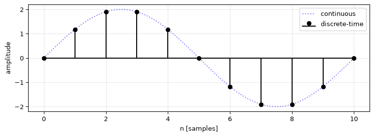
A discrete-time signal is typically plotted as vertical lines (a “stem plot”), emphasising that values exist only at integer sample indices, with nothing in between.
import numpy as npimport matplotlib.pyplot as pltfs =10_000# sampling frequency [Hz]f0 =1_000# signal frequency [Hz]A =2.0# amplitudeN =11# number of samples to shown = np.arange(N) # sample indicess = A * np.sin(2* np.pi * f0 * n / fs)# high-resolution "continuous" version for referencet_cont = np.linspace(0, N -1, 1000)s_cont = A * np.sin(2* np.pi * (f0 / fs) * t_cont)fig, ax = plt.subplots(figsize=(8, 3))ax.plot(t_cont, s_cont, 'b:', alpha=0.5, label='continuous')ax.stem(n, s, linefmt='k-', markerfmt='ko', basefmt='k-', label='discrete-time')ax.set_xlabel('n [samples]')ax.set_ylabel('amplitude')ax.legend()ax.grid(True, alpha=0.3)plt.tight_layout()plt.show()
Figure 1: A continuous sinusoid (dashed) and its sampled version (stems).
Representing sequences
Any discrete-time signal can be written as a weighted sum of shifted impulses. The Kronecker delta is the building block:
This representation is useful because it lets us describe any signal as a sum of shifted and scaled unit impulses, a key idea that underpins convolution and filtering later on.
The other fundamental building block is the unit step:
\[u[n] = \begin{cases} 1 & \text{if } n \geq 0 \\ 0 & \text{if } n < 0 \end{cases}\]
The unit step “switches on” at \(n = 0\). It is related to the Kronecker delta by \(\delta[n] = u[n] - u[n-1]\); the delta is the first difference of the step. The unit step appears constantly in DSP: it describes causal signals (signals that start at some point and continue), step responses of systems, and windowing operations.
Signal energy and power
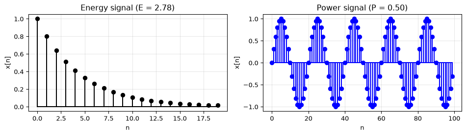
Two quantities tell us about the “size” of a signal. The energy of a discrete-time signal is:
\[E = \sum_{n=-\infty}^{\infty} |x[n]|^2\]
If \(E\) is finite, we call \(x[n]\) an energy signal. A short burst or a decaying pulse has finite energy.
If \(E\) is infinite (the signal goes on forever with non-vanishing amplitude), we use average power instead:
A signal with finite, non-zero \(P\) is a power signal. A constant signal, a sinusoid, and random noise are all power signals: they have infinite energy but well-defined average power.
Figure 3: Energy signal (decaying pulse) vs power signal (sinusoid).
These concepts become important when we discuss signal-to-noise ratio, filter gains, and spectral analysis in later chapters.
Quantization
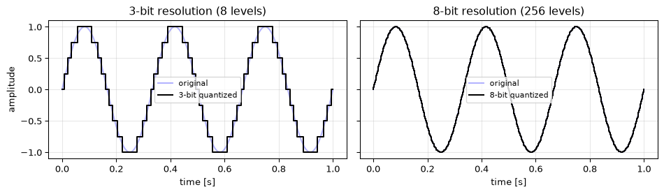
Sampling gives us values at discrete time instants, but those values are still real numbers with infinite precision. Quantization maps each value to the nearest level in a finite set.
An ADC with \(M\)-bit resolution can represent \(2^M\) distinct levels. The voltage resolution (smallest distinguishable step) is:
\[Q = \frac{V_\text{FSR}}{2^M - 1}\]
where \(V_\text{FSR}\) is the full-scale voltage range. The denominator is \(2^M - 1\) because \(2^M\) levels create \(2^M - 1\) intervals.
For example, a 3-bit ADC with a 0–1 V range has \(2^3 = 8\) levels and a resolution of \(Q = 1/7 \approx 0.143\) V. An 8-bit ADC gives 256 levels (\(Q = V_\text{FSR}/255\)); a 16-bit ADC gives 65,536 levels.
The difference between the true value and the quantized value is called quantization error (or quantization noise). For most DSP work, we assume sufficiently high resolution that quantization error is negligible, and we work with the sampled signal as if the values were exact real numbers.
t = np.linspace(0, 1, 500)signal = np.sin(2* np.pi *3* t)def quantize(x, bits):"""Quantize a signal in [-1, 1] to the given bit depth."""# Normalises to [-1, 1]; for voltage resolution see Q = V_FSR / (2^M - 1) above scale =2** (bits -1)return np.clip(np.round(x * scale) / scale, -1.0, 1.0)fig, axes = plt.subplots(1, 2, figsize=(10, 3), sharey=True)for ax, bits inzip(axes, [3, 8]): q = quantize(signal, bits) ax.plot(t, signal, 'b-', alpha=0.3, label='original') ax.step(t, q, 'k-', where='mid', label=f'{bits}-bit quantized') ax.set_xlabel('time [s]') ax.set_title(f'{bits}-bit resolution ({2**bits} levels)') ax.legend(fontsize=8) ax.grid(True, alpha=0.3)axes[0].set_ylabel('amplitude')plt.tight_layout()plt.show()
Figure 4: Effect of quantization: a sinusoid at 3-bit vs 8-bit resolution.
Aliasing and the Nyquist theorem
Sampling works perfectly, under one condition. The Nyquist-Shannon sampling theorem(Oppenheim and Schafer 2010) states that a signal can be exactly reconstructed from its samples if the sampling frequency is greater than twice the highest frequency in the signal:
\[f_s > 2 f_\text{max}\]
The frequency \(f_\text{nyq} = f_s / 2\) is called the Nyquist frequency. It is the highest frequency that can be faithfully represented at a given sampling rate.
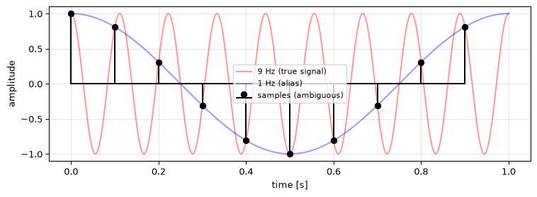
What happens when this condition is violated? Aliasing: frequencies above the Nyquist frequency fold back and appear as lower frequencies in the sampled signal. They are indistinguishable from genuine low-frequency content.
Figure 5: Aliasing: a 9 Hz signal sampled at 10 Hz looks identical to a 1 Hz signal.
Both sinusoids (9 Hz and 1 Hz) pass through exactly the same sample points. Once sampled, there is no way to tell them apart. The 9 Hz signal has been aliased to 1 Hz.
The folding rule
Given a sampling rate \(f_s\), any frequency \(f\) aliases to an apparent frequency in \([0, f_s/2]\). The general rule: fold \(f\) into the interval \([0, f_s]\) by computing \(f \bmod f_s\), then reflect about \(f_s/2\):
For example, \(f = 9\) Hz at \(f_s = 10\) Hz: \(9 \bmod 10 = 9 > 5\), so \(f_\text{alias} = 10 - 9 = 1\) Hz.
Preventing aliasing
In practice, there are two defences:
Anti-aliasing filter: a low-pass analog filter placed before the ADC that removes frequencies above \(f_\text{nyq}\). This is essential hardware; you cannot fix aliasing after sampling.
Oversampling: sampling at a rate much higher than the minimum required, which pushes the aliasing boundary far above the frequencies of interest.
Reconstruction and the DAC
Sampling converts analog to digital. The return path, digital-to-analog conversion, converts the processed samples back to a continuous signal. This is needed whenever the output is physical: driving a speaker, controlling a motor, generating a test waveform.
Zero-order hold
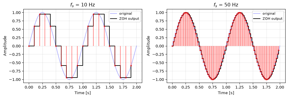
A DAC outputs the value of each sample and holds it constant until the next sample arrives. This is called a zero-order hold (ZOH), and it produces a staircase approximation of the original signal:
Figure 6: Zero-order hold: the DAC output (staircase) approximates the original sinusoid. The steps are clearly visible at low sample rates.
The staircase output is not ideal; the sharp steps contain high-frequency energy that was not in the original signal. In the frequency domain, the ZOH introduces a sinc roll-off: frequencies near Nyquist are attenuated, and spectral images (copies of the baseband spectrum) appear at multiples of \(f_s\).
Anti-imaging filter
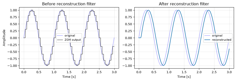
Just as aliasing creates false low-frequency components on the input side, the DAC creates spectral images: copies of the signal spectrum centred at \(f_s\), \(2f_s\), etc. An anti-imaging filter (also called a reconstruction filter) is an analog lowpass placed after the DAC to remove these images, leaving only the original baseband signal.
Figure 7: Reconstruction: the ZOH staircase (left) is smoothed by an anti-imaging lowpass filter (right), recovering an approximation of the original signal.
The combination of ZOH + anti-imaging filter recovers a smooth signal that closely approximates the original. The higher the sample rate, the easier the reconstruction filter’s job: it has a wider transition band to work with.
Oversampling on the output side
Just as oversampling on the input relaxes the anti-aliasing filter, oversampling on the output relaxes the anti-imaging filter. Modern audio DACs internally upsample to 4× or 8× the original rate, then use a gentle analog filter to remove the images. This is why a CD player (\(f_s = 44.1\) kHz) can use a simple output filter rather than a brick-wall filter at 22 kHz.
The complete DSP system
A typical DSP system has five stages, three on input and two on output:
Digital processor: the actual signal processing (filtering, analysis, etc.)
DAC: converts samples back to a staircase analog signal (ZOH)
Anti-imaging filter (analog lowpass): smooths the staircase, removes spectral images
When the input is already digital (a file, a data stream), stages 1–2 are skipped. When the output stays digital (stored, transmitted), stages 4–5 are skipped.
Figure 8: A typical DSP signal chain.
Summary
A signal is a function carrying information about a system.
Sampling converts a continuous signal to a sequence of numbers at regular intervals.
The Kronecker delta\(\delta[n]\) and unit step\(u[n]\) are the fundamental building blocks for discrete-time signals.
Energy signals have finite \(E = \sum |x[n]|^2\); power signals have finite average power \(P\).
Quantization rounds each sample to a finite set of values.
The Nyquist theorem requires \(f_s > 2 f_\text{max}\) to avoid aliasing.
Aliasing folds high frequencies into low frequencies. It cannot be undone after sampling.
An anti-aliasing filter before the ADC is essential in any practical system.
Reconstruction uses a DAC (zero-order hold) followed by an anti-imaging filter to recover a smooth analog output.
Oversampling (on input or output) relaxes the analog filter requirements.
Exercises
Exercise 1.1: Signal classification
Classify each of the following signals as time-discrete, amplitude-discrete, or digital (both):
Number of rainy days per month
Outdoor temperature
Average temperature per month
Population of China
Daily milk production of a farm
Solution
Digital: time-discrete (one value per month) and amplitude-discrete (integer count)
Neither: continuous in both time and amplitude (analog signal)
Time-discrete: one value per month, but amplitude is continuous (could be 14.37 °C)
Amplitude-discrete: integer number of people, but changes continuously in time (births/deaths happen at arbitrary times)
Time-discrete: one measurement per day, but the volume itself is a continuous quantity
Exercise 1.2: Sampling parameters
A sensor samples temperature at \(f_s = 50\) Hz.
What is the sampling period \(T\)?
How many samples are collected in 3 seconds?
What is the highest frequency that can be represented without aliasing?
fs =50T =1/ fsN = fs *3f_nyq = fs /2print(f"Sampling period: T = {T*1000:.0f} ms")print(f"Samples in 3 s: N = {N}")print(f"Nyquist frequency: f_nyq = {f_nyq} Hz")
Sampling period:    T = 20 ms
Samples in 3 s:     N = 150
Nyquist frequency:  f_nyq = 25.0 Hz
Exercise 1.3: Aliasing
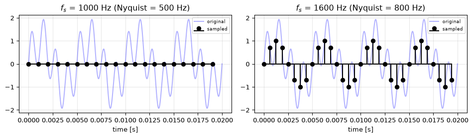
A signal contains two sinusoidal components at 200 Hz and 800 Hz. It is sampled at \(f_s = 1000\) Hz.
Which frequency components will be present in the sampled signal?
Now reduce the sampling rate to \(f_s = 500\) Hz. What happens?
At what minimum sampling rate would both components be preserved?
Solution
Nyquist frequency is \(f_s/2 = 500\) Hz. The 200 Hz component is below Nyquist, so no aliasing. But 800 Hz is above 500 Hz. Applying the folding rule: \(800 \bmod 1000 = 800\); since \(800 > 500\): \(f_\text{alias} = 1000 - 800 = 200\) Hz. The sampled signal contains a 200 Hz component (the original 200 Hz and the aliased 800 Hz overlap; the resulting amplitude depends on their relative phase).
At \(f_s = 500\) Hz, Nyquist is 250 Hz. The 200 Hz component survives. For 800 Hz: \(800 \bmod 500 = 300\); since \(300 > 250\): \(f_\text{alias} = 500 - 300 = 200\) Hz. Again both components alias to 200 Hz.
Calculate the voltage resolution \(Q\) for 8-bit, 12-bit, and 16-bit converters.
A temperature sensor outputs 10 mV/°C. What is the smallest temperature change each ADC can detect?
Which resolution would you choose for a medical thermometer that needs 0.01 °C accuracy?
Solution
\[Q = \frac{V_\text{FSR}}{2^M - 1}\]
With sensitivity 10 mV/°C, the temperature resolution is \(\Delta T = Q / 0.010\).
We need \(\Delta T \leq 0.01\) °C, so \(Q \leq 0.1\) mV. The 16-bit ADC (\(\approx\) 0.050 mV) is the only one that meets this requirement. The 12-bit ADC (\(\approx\) 0.806 mV → 0.081 °C) falls short.
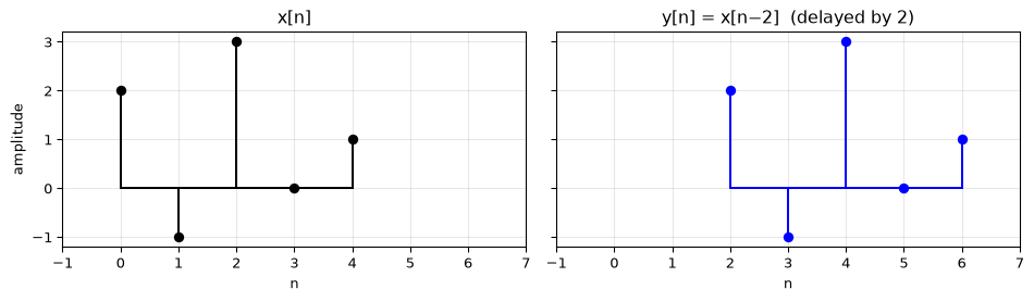
import numpy as npimport matplotlib.pyplot as pltx = np.array([2, -1, 3, 0, 1])n_x = np.arange(len(x))# y[n] = x[n-2]: shift right by 2y = x.copy()n_y = n_x +2fig, axes = plt.subplots(1, 2, figsize=(10, 3), sharey=True)axes[0].stem(n_x, x, linefmt='k-', markerfmt='ko', basefmt='k-')axes[0].set_xlabel('n')axes[0].set_ylabel('amplitude')axes[0].set_title('x[n]')axes[0].set_xlim(-1, 7)axes[0].grid(True, alpha=0.3)axes[1].stem(n_y, y, linefmt='b-', markerfmt='bo', basefmt='b-')axes[1].set_xlabel('n')axes[1].set_title('y[n] = x[n−2] (delayed by 2)')axes[1].set_xlim(-1, 7)axes[1].grid(True, alpha=0.3)plt.tight_layout()plt.show()
\(y[n] = x[n-2]\) means \(y[2]=2\), \(y[3]=-1\), \(y[4]=3\), \(y[5]=0\), \(y[6]=1\). The signal is delayed (shifted right) by 2 samples. The shape is identical; only the timing changed.
Want more practice? See the Exercise set for Chapter 1 for additional problems at varying difficulty levels.
The next chapter takes the sampled signal and introduces the systems that process it: Discrete-time systems.
Further reading
Oppenheim & Schafer, Discrete-Time Signal Processing (2010), Ch. 4.1–4.3: Sampling and reconstruction
Proakis & Manolakis, Digital Signal Processing (2007), Ch. 1.3–1.5: A/D conversion, quantization
References
Oppenheim, Alan V., and Ronald W. Schafer. 2010. Discrete-Time Signal Processing. 3rd ed. Pearson.
Source Code
---title: "Signals and Sampling"subtitle: "From the physical world to numbers in memory"---## What is digital signal processing?Digital signal processing (DSP) is about working with signals (measurements that vary over time or space) using computers. The "digital" part means we work with numbers, not voltages.DSP is everywhere. Your phone uses it for voice calls, noise cancellation, and music playback. Medical devices use it to clean up ECG and EEG signals. Cars use it for radar and motor control. Scientific instruments use it for everything from radio telescopes to environmental monitoring.| Domain | Examples ||--------|----------|| Communication | Digital telephony, data compression, echo cancellation || Medical | Patient monitoring, diagnostic imaging (MRI, ultrasound) || Automotive | Radar, lidar, motor control, ADAS || Science | Data acquisition, spectral analysis, environmental monitoring || Entertainment | Audio processing, video compression, streaming |The reason DSP has displaced analog processing in most applications comes down to one thing: **noise resilience**. An analog signal degrades every time it's copied, transmitted, or processed. A digital signal (a sequence of numbers) can be copied perfectly and processed with arbitrary precision.## SignalsIn engineering, a **signal** is a function representing some variable that carries information about a system. A temperature reading, a microphone voltage, an accelerometer output: these are all signals.Signals are meaningless without systems to interpret them, and systems are useless without signals to process. Before we can build a processing system, we need to understand how signals become digital.## From continuous to discrete: samplingTo process an analog (continuous-time) signal digitally, we need to convert it to numbers. An **analog-to-digital converter** (ADC) does this in two steps:1. **Sampling**: measure the signal at regular time intervals2. **Quantization**: round each measurement to a finite set of valuesLet's focus on sampling first.### The sampling processLet $s(t)$ be a continuous signal. Sampling means measuring its value every $T$ seconds (the **sampling period**). The result is a sequence of numbers:$$s[n] = s(nT), \quad n \in \mathbb{Z}$$where $n$ is the sample number. The **sampling frequency** (or sampling rate) is:$$f_s = \frac{1}{T}$$A discrete-time signal is typically plotted as vertical lines (a "stem plot"), emphasising that values exist only at integer sample indices, with nothing in between.```{python}#| label: fig-stem#| fig-cap: "A continuous sinusoid (dashed) and its sampled version (stems)."import numpy as npimport matplotlib.pyplot as pltfs =10_000# sampling frequency [Hz]f0 =1_000# signal frequency [Hz]A =2.0# amplitudeN =11# number of samples to shown = np.arange(N) # sample indicess = A * np.sin(2* np.pi * f0 * n / fs)# high-resolution "continuous" version for referencet_cont = np.linspace(0, N -1, 1000)s_cont = A * np.sin(2* np.pi * (f0 / fs) * t_cont)fig, ax = plt.subplots(figsize=(8, 3))ax.plot(t_cont, s_cont, 'b:', alpha=0.5, label='continuous')ax.stem(n, s, linefmt='k-', markerfmt='ko', basefmt='k-', label='discrete-time')ax.set_xlabel('n [samples]')ax.set_ylabel('amplitude')ax.legend()ax.grid(True, alpha=0.3)plt.tight_layout()plt.show()```### Representing sequencesAny discrete-time signal can be written as a weighted sum of shifted impulses. The **Kronecker delta** is the building block:$$\delta[n] = \begin{cases} 1 & \text{if } n = 0 \\ 0 & \text{otherwise} \end{cases}$$A sequence like $x[0] = 0.5$, $x[1] = 3.0$, $x[2] = -0.5$, $x[3] = 1.0$ can be expressed as:$$x[n] = 0.5\,\delta[n] + 3.0\,\delta[n-1] - 0.5\,\delta[n-2] + 1.0\,\delta[n-3]$$This representation is useful because it lets us describe any signal as a sum of shifted and scaled unit impulses, a key idea that underpins convolution and filtering later on.```{python}#| label: fig-sequence#| fig-cap: "A simple four-sample sequence."x = np.array([0.5, 3.0, -0.5, 1.0])n = np.arange(len(x))fig, ax = plt.subplots(figsize=(6, 3))ax.stem(n, x, linefmt='k-', markerfmt='ko', basefmt='k-')ax.set_xlabel('n [samples]')ax.set_ylabel('x[n]')ax.set_xlim(-0.5, 4.5)ax.set_ylim(-1.5, 4.0)ax.grid(True, alpha=0.3)plt.tight_layout()plt.show()```### The unit stepThe other fundamental building block is the **unit step**:$$u[n] = \begin{cases} 1 & \text{if } n \geq 0 \\ 0 & \text{if } n < 0 \end{cases}$$The unit step "switches on" at $n = 0$. It is related to the Kronecker delta by $\delta[n] = u[n] - u[n-1]$; the delta is the first difference of the step. The unit step appears constantly in DSP: it describes causal signals (signals that start at some point and continue), step responses of systems, and windowing operations.### Signal energy and powerTwo quantities tell us about the "size" of a signal. The **energy** of a discrete-time signal is:$$E = \sum_{n=-\infty}^{\infty} |x[n]|^2$$If $E$ is finite, we call $x[n]$ an **energy signal**. A short burst or a decaying pulse has finite energy.If $E$ is infinite (the signal goes on forever with non-vanishing amplitude), we use **average power** instead:$$P = \lim_{N \to \infty} \frac{1}{2N+1} \sum_{n=-N}^{N} |x[n]|^2$$A signal with finite, non-zero $P$ is a **power signal**. A constant signal, a sinusoid, and random noise are all power signals: they have infinite energy but well-defined average power.```{python}#| label: fig-energy-power#| fig-cap: "Energy signal (decaying pulse) vs power signal (sinusoid)."n_pulse = np.arange(20)pulse =0.8** n_pulse # decaying exponential — finite energyn_sine = np.arange(100)sine = np.sin(2* np.pi *0.05* n_sine) # sinusoid — finite powerfig, axes = plt.subplots(1, 2, figsize=(10, 3))axes[0].stem(n_pulse, pulse, linefmt='k-', markerfmt='ko', basefmt='k-')E = np.sum(pulse **2)axes[0].set_title(f'Energy signal (E = {E:.2f})')axes[0].set_xlabel('n')axes[0].set_ylabel('x[n]')axes[0].grid(True, alpha=0.3)axes[1].stem(n_sine, sine, linefmt='b-', markerfmt='bo', basefmt='b-', label='signal')P = np.mean(sine **2)axes[1].set_title(f'Power signal (P = {P:.2f})')axes[1].set_xlabel('n')axes[1].set_ylabel('x[n]')axes[1].grid(True, alpha=0.3)plt.tight_layout()plt.show()```These concepts become important when we discuss signal-to-noise ratio, filter gains, and spectral analysis in later chapters.## QuantizationSampling gives us values at discrete time instants, but those values are still real numbers with infinite precision. **Quantization** maps each value to the nearest level in a finite set.An ADC with $M$-bit resolution can represent $2^M$ distinct levels. The **voltage resolution** (smallest distinguishable step) is:$$Q = \frac{V_\text{FSR}}{2^M - 1}$$where $V_\text{FSR}$ is the full-scale voltage range. The denominator is $2^M - 1$ because $2^M$ levels create $2^M - 1$ intervals.For example, a 3-bit ADC with a 0–1 V range has $2^3 = 8$ levels and a resolution of $Q = 1/7 \approx 0.143$ V. An 8-bit ADC gives 256 levels ($Q = V_\text{FSR}/255$); a 16-bit ADC gives 65,536 levels.The difference between the true value and the quantized value is called **quantization error** (or quantization noise). For most DSP work, we assume sufficiently high resolution that quantization error is negligible, and we work with the sampled signal as if the values were exact real numbers.```{python}#| label: fig-quantization#| fig-cap: "Effect of quantization: a sinusoid at 3-bit vs 8-bit resolution."t = np.linspace(0, 1, 500)signal = np.sin(2* np.pi *3* t)def quantize(x, bits):"""Quantize a signal in [-1, 1] to the given bit depth."""# Normalises to [-1, 1]; for voltage resolution see Q = V_FSR / (2^M - 1) above scale =2** (bits -1)return np.clip(np.round(x * scale) / scale, -1.0, 1.0)fig, axes = plt.subplots(1, 2, figsize=(10, 3), sharey=True)for ax, bits inzip(axes, [3, 8]): q = quantize(signal, bits) ax.plot(t, signal, 'b-', alpha=0.3, label='original') ax.step(t, q, 'k-', where='mid', label=f'{bits}-bit quantized') ax.set_xlabel('time [s]') ax.set_title(f'{bits}-bit resolution ({2**bits} levels)') ax.legend(fontsize=8) ax.grid(True, alpha=0.3)axes[0].set_ylabel('amplitude')plt.tight_layout()plt.show()```## Aliasing and the Nyquist theoremSampling works perfectly, under one condition. The **Nyquist-Shannon sampling theorem** [@oppenheim2010discrete] states that a signal can be exactly reconstructed from its samples if the sampling frequency is greater than twice the highest frequency in the signal:$$f_s > 2 f_\text{max}$$The frequency $f_\text{nyq} = f_s / 2$ is called the **Nyquist frequency**. It is the highest frequency that can be faithfully represented at a given sampling rate.What happens when this condition is violated? **Aliasing**: frequencies above the Nyquist frequency fold back and appear as lower frequencies in the sampled signal. They are indistinguishable from genuine low-frequency content.```{python}#| label: fig-aliasing#| fig-cap: "Aliasing: a 9 Hz signal sampled at 10 Hz looks identical to a 1 Hz signal."fs =10# sampling frequencyn = np.arange(10)t_fine = np.linspace(0, 1, 1000)f_true =9# above Nyquistf_alias =1# what it looks like after samplingfig, ax = plt.subplots(figsize=(8, 3))ax.plot(t_fine, np.cos(2* np.pi * f_true * t_fine), 'r-', alpha=0.4, label=f'{f_true} Hz (true signal)')ax.plot(t_fine, np.cos(2* np.pi * f_alias * t_fine), 'b-', alpha=0.4, label=f'{f_alias} Hz (alias)')ax.stem(n / fs, np.cos(2* np.pi * f_true * n / fs), linefmt='k-', markerfmt='ko', basefmt='k-', label='samples (ambiguous)')ax.set_xlabel('time [s]')ax.set_ylabel('amplitude')ax.legend(fontsize=8)ax.grid(True, alpha=0.3)plt.tight_layout()plt.show()```Both sinusoids (9 Hz and 1 Hz) pass through exactly the same sample points. Once sampled, there is no way to tell them apart. The 9 Hz signal has been **aliased** to 1 Hz.### The folding ruleGiven a sampling rate $f_s$, any frequency $f$ aliases to an apparent frequency in $[0, f_s/2]$. The general rule: fold $f$ into the interval $[0, f_s]$ by computing $f \bmod f_s$, then reflect about $f_s/2$:$$f_\text{alias} = \begin{cases} f \bmod f_s & \text{if } (f \bmod f_s) \leq f_s/2 \\ f_s - (f \bmod f_s) & \text{if } (f \bmod f_s) > f_s/2 \end{cases}$$For example, $f = 9$ Hz at $f_s = 10$ Hz: $9 \bmod 10 = 9 > 5$, so $f_\text{alias} = 10 - 9 = 1$ Hz.### Preventing aliasingIn practice, there are two defences:1. **Anti-aliasing filter**: a low-pass analog filter placed before the ADC that removes frequencies above $f_\text{nyq}$. This is essential hardware; you cannot fix aliasing after sampling.2. **Oversampling**: sampling at a rate much higher than the minimum required, which pushes the aliasing boundary far above the frequencies of interest.## Reconstruction and the DACSampling converts analog to digital. The return path, **digital-to-analog conversion**, converts the processed samples back to a continuous signal. This is needed whenever the output is physical: driving a speaker, controlling a motor, generating a test waveform.### Zero-order holdA DAC outputs the value of each sample and holds it constant until the next sample arrives. This is called a **zero-order hold** (ZOH), and it produces a staircase approximation of the original signal:```{python}#| label: fig-zoh#| fig-cap: "Zero-order hold: the DAC output (staircase) approximates the original sinusoid. The steps are clearly visible at low sample rates."fs_low, fs_high =10, 50f0 =1# Hzt_fine = np.linspace(0, 2, 2000)s_fine = np.sin(2* np.pi * f0 * t_fine)fig, axes = plt.subplots(1, 2, figsize=(10, 3.5))for ax, fs inzip(axes, [fs_low, fs_high]): n = np.arange(int(2* fs)) t_samples = n / fs s_samples = np.sin(2* np.pi * f0 * t_samples) ax.plot(t_fine, s_fine, 'b-', alpha=0.3, label='original') ax.step(t_samples, s_samples, 'k-', where='post', linewidth=1.5, label='ZOH output') markerline, stemlines, baseline = ax.stem(t_samples, s_samples, linefmt='r-', markerfmt='r.', basefmt=' ') plt.setp(stemlines, alpha=0.5) plt.setp(markerline, alpha=0.5) ax.set_xlabel('Time [s]') ax.set_ylabel('Amplitude') ax.set_title(f'$f_s$ = {fs} Hz') ax.legend(fontsize=8) ax.grid(True, alpha=0.3)fig.tight_layout()plt.show()```The staircase output is not ideal; the sharp steps contain high-frequency energy that was not in the original signal. In the frequency domain, the ZOH introduces a **sinc roll-off**: frequencies near Nyquist are attenuated, and spectral images (copies of the baseband spectrum) appear at multiples of $f_s$.### Anti-imaging filterJust as aliasing creates false low-frequency components on the input side, the DAC creates **spectral images**: copies of the signal spectrum centred at $f_s$, $2f_s$, etc. An **anti-imaging filter** (also called a reconstruction filter) is an analog lowpass placed after the DAC to remove these images, leaving only the original baseband signal.```{python}#| label: fig-reconstruction#| fig-cap: "Reconstruction: the ZOH staircase (left) is smoothed by an anti-imaging lowpass filter (right), recovering an approximation of the original signal."from scipy.signal import butter, sosfiltfs =20f0 =1duration =3n = np.arange(int(duration * fs))t_samples = n / fss_samples = np.sin(2* np.pi * f0 * t_samples)# Simulate ZOH by upsampling + holdingupsample =100t_zoh = np.arange(len(n) * upsample) / (fs * upsample)s_zoh = np.repeat(s_samples, upsample)# Anti-imaging filter (lowpass at Nyquist)sos = butter(4, fs /2, fs=fs * upsample, output='sos')s_reconstructed = sosfilt(sos, s_zoh)# True signalt_fine = np.linspace(0, duration, 5000)s_fine = np.sin(2* np.pi * f0 * t_fine)fig, axes = plt.subplots(1, 2, figsize=(10, 3.5))axes[0].plot(t_fine, s_fine, 'b-', alpha=0.3, label='original')axes[0].plot(t_zoh, s_zoh, 'k-', linewidth=0.8, label='ZOH output')axes[0].set_title('Before reconstruction filter')axes[0].set_xlabel('Time [s]')axes[0].set_ylabel('Amplitude')axes[0].legend(fontsize=8)axes[0].grid(True, alpha=0.3)axes[1].plot(t_fine, s_fine, 'b-', alpha=0.3, label='original')axes[1].plot(t_zoh, s_reconstructed, 'C0-', linewidth=1.5, label='reconstructed')axes[1].set_title('After reconstruction filter')axes[1].set_xlabel('Time [s]')axes[1].legend(fontsize=8)axes[1].grid(True, alpha=0.3)fig.tight_layout()plt.show()```The combination of ZOH + anti-imaging filter recovers a smooth signal that closely approximates the original. The higher the sample rate, the easier the reconstruction filter's job: it has a wider transition band to work with.### Oversampling on the output sideJust as oversampling on the input relaxes the anti-aliasing filter, **oversampling on the output** relaxes the anti-imaging filter. Modern audio DACs internally upsample to 4× or 8× the original rate, then use a gentle analog filter to remove the images. This is why a CD player ($f_s = 44.1$ kHz) can use a simple output filter rather than a brick-wall filter at 22 kHz.## The complete DSP systemA typical DSP system has five stages, three on input and two on output:1. **Anti-aliasing filter** (analog lowpass): removes frequencies above $f_\text{nyq}$2. **ADC**: samples and quantizes the filtered signal3. **Digital processor**: the actual signal processing (filtering, analysis, etc.)4. **DAC**: converts samples back to a staircase analog signal (ZOH)5. **Anti-imaging filter** (analog lowpass): smooths the staircase, removes spectral imagesWhen the input is already digital (a file, a data stream), stages 1–2 are skipped. When the output stays digital (stored, transmitted), stages 4–5 are skipped.```{dot}//| echo: false//| label: fig-dsp-chain//| fig-cap: "A typical DSP signal chain."digraph { rankdir=LR graph [pad=0 margin=0] node [fontname="sans-serif" fontsize=14 shape=box height=0.4 margin="0.1,0.05"] edge [arrowsize=0.8] xt [label="x(t)" shape=plaintext fontname="serif"] AAF [label="AAF"] ADC [label="ADC"] DSP [label="DSP"] DAC [label="DAC"] yt [label="y(t)" shape=plaintext fontname="serif"] xt -> AAF -> ADC -> DSP -> DAC -> yt}```## Summary- A **signal** is a function carrying information about a system.- **Sampling** converts a continuous signal to a sequence of numbers at regular intervals.- The **Kronecker delta** $\delta[n]$ and **unit step** $u[n]$ are the fundamental building blocks for discrete-time signals.- **Energy signals** have finite $E = \sum |x[n]|^2$; **power signals** have finite average power $P$.- **Quantization** rounds each sample to a finite set of values.- The **Nyquist theorem** requires $f_s > 2 f_\text{max}$ to avoid aliasing.- **Aliasing** folds high frequencies into low frequencies. It cannot be undone after sampling.- An **anti-aliasing filter** before the ADC is essential in any practical system.- **Reconstruction** uses a DAC (zero-order hold) followed by an **anti-imaging filter** to recover a smooth analog output.- **Oversampling** (on input or output) relaxes the analog filter requirements.## Exercises::: {.callout-tip collapse="true" title="Exercise 1.1: Signal classification"}Classify each of the following signals as **time-discrete**, **amplitude-discrete**, or **digital** (both):1. Number of rainy days per month2. Outdoor temperature3. Average temperature per month4. Population of China5. Daily milk production of a farm::: {.callout-note collapse="true" title="Solution"}1. **Digital**: time-discrete (one value per month) and amplitude-discrete (integer count)2. **Neither**: continuous in both time and amplitude (analog signal)3. **Time-discrete**: one value per month, but amplitude is continuous (could be 14.37 °C)4. **Amplitude-discrete**: integer number of people, but changes continuously in time (births/deaths happen at arbitrary times)5. **Time-discrete**: one measurement per day, but the volume itself is a continuous quantity::::::::: {.callout-tip collapse="true" title="Exercise 1.2: Sampling parameters"}A sensor samples temperature at $f_s = 50$ Hz.a) What is the sampling period $T$?b) How many samples are collected in 3 seconds?c) What is the highest frequency that can be represented without aliasing?::: {.callout-note collapse="true" title="Solution"}a) $T = 1/f_s = 1/50 = 0.02$ s = 20 msb) $N = f_s \times t = 50 \times 3 = 150$ samplesc) The Nyquist frequency: $f_\text{nyq} = f_s / 2 = 25$ Hz```{python}fs =50T =1/ fsN = fs *3f_nyq = fs /2print(f"Sampling period: T = {T*1000:.0f} ms")print(f"Samples in 3 s: N = {N}")print(f"Nyquist frequency: f_nyq = {f_nyq} Hz")```::::::::: {.callout-tip collapse="true" title="Exercise 1.3: Aliasing"}A signal contains two sinusoidal components at 200 Hz and 800 Hz. It is sampled at $f_s = 1000$ Hz.a) Which frequency components will be present in the sampled signal?b) Now reduce the sampling rate to $f_s = 500$ Hz. What happens?c) At what minimum sampling rate would both components be preserved?::: {.callout-note collapse="true" title="Solution"}a) Nyquist frequency is $f_s/2 = 500$ Hz. The 200 Hz component is below Nyquist, so no aliasing. But 800 Hz is *above* 500 Hz. Applying the folding rule: $800 \bmod 1000 = 800$; since $800 > 500$: $f_\text{alias} = 1000 - 800 = 200$ Hz. The sampled signal contains a 200 Hz component (the original 200 Hz and the aliased 800 Hz overlap; the resulting amplitude depends on their relative phase).b) At $f_s = 500$ Hz, Nyquist is 250 Hz. The 200 Hz component survives. For 800 Hz: $800 \bmod 500 = 300$; since $300 > 250$: $f_\text{alias} = 500 - 300 = 200$ Hz. Again both components alias to 200 Hz.c) $f_s > 2 \times 800 = 1600$ Hz.```{python}import numpy as npimport matplotlib.pyplot as pltf1, f2 =200, 800t_fine = np.linspace(0, 0.02, 2000)signal = np.sin(2* np.pi * f1 * t_fine) + np.sin(2* np.pi * f2 * t_fine)fig, axes = plt.subplots(1, 2, figsize=(10, 3))for ax, fs inzip(axes, [1000, 1600]): n = np.arange(int(fs *0.02)) t_samples = n / fs sampled = np.sin(2* np.pi * f1 * t_samples) + np.sin(2* np.pi * f2 * t_samples) ax.plot(t_fine, signal, 'b-', alpha=0.3, label='original') ax.stem(t_samples, sampled, linefmt='k-', markerfmt='ko', basefmt='k-', label='sampled') ax.set_title(f'$f_s$ = {fs} Hz (Nyquist = {fs//2} Hz)') ax.set_xlabel('time [s]') ax.legend(fontsize=7) ax.grid(True, alpha=0.3)plt.tight_layout()plt.show()```::::::::: {.callout-tip collapse="true" title="Exercise 1.4: Quantization resolution"}An ADC has a 0–3.3 V input range.a) Calculate the voltage resolution $Q$ for 8-bit, 12-bit, and 16-bit converters.b) A temperature sensor outputs 10 mV/°C. What is the smallest temperature change each ADC can detect?c) Which resolution would you choose for a medical thermometer that needs 0.01 °C accuracy?::: {.callout-note collapse="true" title="Solution"}a)$$Q = \frac{V_\text{FSR}}{2^M - 1}$$b) With sensitivity 10 mV/°C, the temperature resolution is $\Delta T = Q / 0.010$.c) We need $\Delta T \leq 0.01$ °C, so $Q \leq 0.1$ mV. The 16-bit ADC ($\approx$ 0.050 mV) is the only one that meets this requirement. The 12-bit ADC ($\approx$ 0.806 mV → 0.081 °C) falls short.```{python}V_FSR =3.3# full-scale range [V]sensitivity =0.010# 10 mV/°Cprint(f"{'Bits':>4s}{'Levels':>6s}{'Q [mV]':>8s}{'ΔT [°C]':>8s}")print("-"*34)for bits in [8, 12, 16]: levels =2** bits Q = V_FSR / (levels -1) delta_T = Q / sensitivityprint(f"{bits:4d}{levels:6d}{Q*1000:8.3f}{delta_T:8.3f}")```::::::::: {.callout-tip collapse="true" title="Exercise 1.5: Sequence representation"}Given the signal $x[n]$ defined by the samples: $x[0]=2$, $x[1]=-1$, $x[2]=3$, $x[3]=0$, $x[4]=1$.a) Write $x[n]$ as a sum of weighted Kronecker deltas.b) Plot the sequence as a stem plot.c) A second signal is defined as $y[n] = x[n-2]$. What are the values of $y[n]$ and what happened to the signal?::: {.callout-note collapse="true" title="Solution"}a) $x[n] = 2\,\delta[n] - 1\,\delta[n-1] + 3\,\delta[n-2] + 0\,\delta[n-3] + 1\,\delta[n-4]$b)```{python}import numpy as npimport matplotlib.pyplot as pltx = np.array([2, -1, 3, 0, 1])n_x = np.arange(len(x))# y[n] = x[n-2]: shift right by 2y = x.copy()n_y = n_x +2fig, axes = plt.subplots(1, 2, figsize=(10, 3), sharey=True)axes[0].stem(n_x, x, linefmt='k-', markerfmt='ko', basefmt='k-')axes[0].set_xlabel('n')axes[0].set_ylabel('amplitude')axes[0].set_title('x[n]')axes[0].set_xlim(-1, 7)axes[0].grid(True, alpha=0.3)axes[1].stem(n_y, y, linefmt='b-', markerfmt='bo', basefmt='b-')axes[1].set_xlabel('n')axes[1].set_title('y[n] = x[n−2] (delayed by 2)')axes[1].set_xlim(-1, 7)axes[1].grid(True, alpha=0.3)plt.tight_layout()plt.show()```c) $y[n] = x[n-2]$ means $y[2]=2$, $y[3]=-1$, $y[4]=3$, $y[5]=0$, $y[6]=1$. The signal is **delayed** (shifted right) by 2 samples. The shape is identical; only the timing changed.::::::Want more practice? See the [Exercise set for Chapter 1](../exercises/01-signals.qmd) for additional problems at varying difficulty levels.The next chapter takes the sampled signal and introduces the systems that process it: [Discrete-time systems](02-discrete-time.qmd).::: {.callout-note title="Further reading"}- Oppenheim & Schafer, *Discrete-Time Signal Processing* (2010), Ch. 4.1–4.3: Sampling and reconstruction- Proakis & Manolakis, *Digital Signal Processing* (2007), Ch. 1.3–1.5: A/D conversion, quantization:::## References::: {#refs}:::