Moving average and exponential smoothing on ESP32-S3 and STM32F4
Smoothing is often the first DSP operation applied to sensor data on a microcontroller, before peak detection, zero-crossing analysis, or any downstream processing. The moving average and exponential moving average (EMA) are trivially cheap to implement and cover the majority of embedded smoothing needs.
For the theory (frequency response, Savitzky-Golay, kernel smoothing, trade-offs), see the main smoothing page.
Exponential moving average (EMA)
The EMA is the simplest recursive smoother and the most commonly used on microcontrollers. As written below it costs two multiplies and one addition (it can be factored to \(y[n] = x[n] + \alpha\,(y[n-1] - x[n])\) for one multiply, one subtract, and one add, trading a multiply for a cheaper add), with a single state variable:
Note the convention: here \(\alpha\) weights the previous output, so \(\alpha\) near 1 means heavy smoothing, the opposite of the main page’s smoothing-factor \(\alpha\) (which weights the new sample, small \(\alpha\) = heavy smoothing). They relate by \(\alpha_\text{here} = 1 - \alpha_\text{main}\).
The time constant is \(\tau = -1 / \ln(\alpha)\) samples. For \(\alpha = 0.9\) at 100 Hz sample rate, \(\tau \approx 9.5\) samples (95 ms). For \(\alpha = 0.99\), \(\tau \approx 100\) samples (1 s).
Tip
On targets without hardware FPU (e.g., Cortex-M0), the EMA can be implemented in fixed-point with a power-of-two scaling: \(y[n] = y[n-1] - (y[n-1] \gg K) + (x[n] \gg K)\), where \(\alpha = 1 - 2^{-K}\). This requires only shifts and additions, no multiplications.
Moving average with circular buffer
The \(N\)-point moving average requires storing the last \(N\) samples. A circular buffer avoids shifting the entire array on every sample:
typedefstruct{float*buffer;float sum;// running sum for O(1) updateint head;int N;int count;// samples received so far (for startup)} MovingAverage;void ma_init(MovingAverage *f,float*buffer,int N){ f->buffer = buffer; f->sum =0.0f; f->head =0; f->N = N; f->count =0;for(int i =0; i < N; i++) buffer[i]=0.0f;}float ma_process(MovingAverage *f,float x){// Subtract the oldest sample, add the new one f->sum -= f->buffer[f->head]; f->buffer[f->head]= x; f->sum += x; f->head++;if(f->head >= f->N) f->head =0;if(f->count < f->N) f->count++;return(f->count >0)? f->sum / f->count :0.0f;}
The running-sum trick makes the moving average O(1) per sample regardless of window size: one subtraction, one addition, and one division. This is the same cost as the EMA but requires \(N\) floats of memory.
Floating-point drift
The running sum accumulates rounding errors over millions of samples. For long-running embedded systems (days or weeks), periodically recompute the sum from scratch: sum = 0; for (i = 0; i < N; i++) sum += buffer[i];. Once per second is sufficient and costs negligible CPU.
Moving average on an FPGA: delay line + accumulator
Like the CIC filter, the moving average’s natural home is gateware. Decomposed as a cascade of a feedforward comb (\(1 - z^{-M}\), delay \(M\)) and a feedback integrator (\(1/(1 - z^{-1})\), delay 1), it maps to almost nothing: an \(M\)-deep shift register, one subtractor, one adder, and one accumulator register. There are no multipliers at all (unless you scale the output by \(1/M\) with a non-power-of-two \(M\); for power-of-two \(M\) the division is a right shift, which is free in gate count). “Free” is a statement about area, not about accuracy: shift_right on a signed value is an arithmetic shift, so it floors rather than rounds and leaves a small DC offset on bipolar data. The finite word-length page quantifies the offset and gives the one-adder fix.
The structure is simpler than the CIC because there is no decimation: every stage runs at the sample rate, so the comb delay really is \(M\) registers deep at the fast clock.
VHDL: parameterised moving average
library ieee;use ieee.std_logic_1164.all;use ieee.numeric_std.all;-- Parameterised moving average: M-tap running-sum accumulator.-- Decomposed as comb (1 - z^-M) -> integrator (1 / (1 - z^-1)).-- Two's-complement wrap-around in the accumulator is INTENTIONAL:-- numeric_std 'signed' addition wraps, and the subtraction of x[n-M]-- cancels the wrap exactly; the same CIC overflow story. Do not saturate.entitymoving_averageisgeneric ( B_IN :positive:=16; -- input word width M :positive:=16; -- window length B_SUM :positive:=20-- = B_IN + ceil(log2 M); here 16 + 4 = 20 );port ( clk :instd_logic; rst :instd_logic; x_in :insigned(B_IN-1downto0); y_out :outsigned(B_SUM-1downto0) -- unscaled running sum (÷ M downstream) );end entity;architecturertlofmoving_averageistype delay_line_t isarray (0to M-1) ofsigned(B_IN-1downto0);signal delay_line : delay_line_t := (others=> (others=>'0'));signal sum :signed(B_SUM-1downto0) := (others=>'0');beginprocess(clk)variable x_old :signed(B_IN-1downto0);variable diff :signed(B_SUM-1downto0);beginifrising_edge(clk) thenif rst ='1'then delay_line <= (others=> (others=>'0')); sum <= (others=>'0'); y_out <= (others=>'0');else x_old := delay_line(M-1); -- x[n-M], about to leave the window-- Shift register: newest sample in at position 0, oldest out at M-1 delay_line(0) <= x_in;for k in1to M-1loop delay_line(k) <= delay_line(k-1);end loop;-- Running sum: s[n] = s[n-1] + x[n] - x[n-M]-- resize sign-extends to the accumulator width; wrap is intentional diff := resize(x_in, B_SUM) - resize(x_old, B_SUM); sum <= sum + diff;-- Register the freshly updated sum, not the signal `sum` itself:-- signal reads inside a process see the pre-edge value, so-- `y_out <= sum;` would lag the accumulator by one extra cycle. y_out <= sum + diff;end if;end if;end process;end architecture;
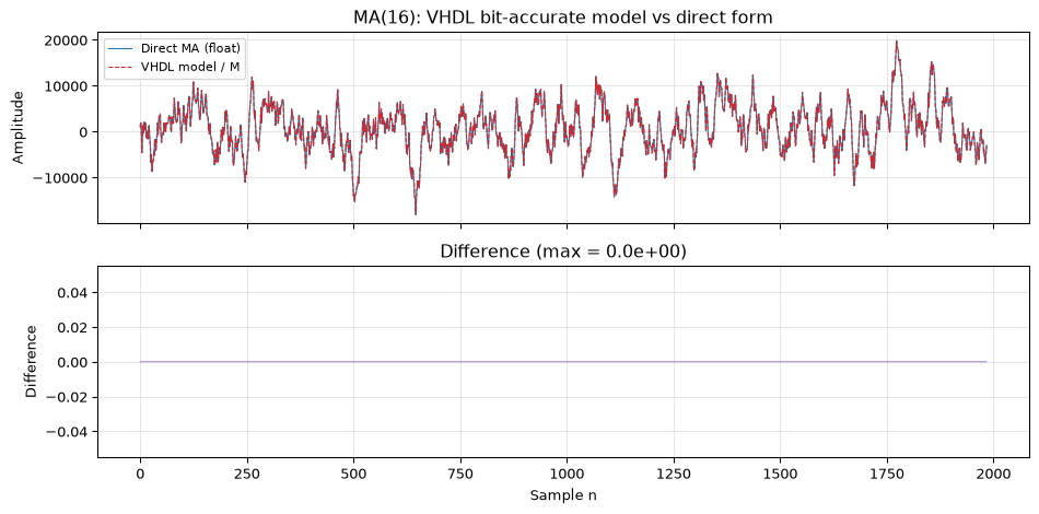
The one design-time number is B_SUM. Size it from \(B_\text{in} + \lceil\log_2 M\rceil\) and this comb-first accumulator never wraps at all: the windowed sum of \(M\) signed \(B_\text{in}\)-bit values is bounded by \(M \cdot 2^{B_\text{in}-1} = 2^{B_\text{SUM}-1}\) by construction. The famous “wrap cancels” guarantee belongs to the integrator-first (CIC) ordering, where the running total does wrap but the comb’s subtraction removes every wrap exactly; the model below proves both facts, and the multirate chapter builds on the CIC form. The output y_out is the unscaled sum. Divide by \(M\) downstream: free when \(M\) is a power of two (right shift), or a single DSP slice otherwise. If you take the right-shift route on signed data, bias the sum by half an output LSB first (add \(2^{k-1}\) before shifting by \(k\)); a bare arithmetic shift floors every sample and biases the smoother’s output low by up to half an LSB, which is exactly the error a level-tracking filter should not have. See scaling by shifts.
Show the code
import numpy as npimport matplotlib.pyplot as pltrng = np.random.default_rng(1)B_IN, M =16, 16B_SUM = B_IN +int(np.ceil(np.log2(M))) # = 20 bitsN_SAMPLES =2000def wrap_signed(v, B):"""Two's-complement wrap to B bits, matching numeric_std signed addition.""" v &= (1<< B) -1return v - (1<< B) if v & (1<< (B -1)) else vdef ma_vhdl(x, wrapping):"""Bit-accurate model of the VHDL moving_average entity.""" delay_line = [0] * M s =0 out = []for xn in x: x_old = delay_line[-1] # x[n-M]# shift register delay_line = [xn] + delay_line[:-1]# accumulator: s += x[n] - x[n-M] diff = xn - x_old s += diffif wrapping: s = wrap_signed(s, B_SUM) out.append(s)return np.array(out, dtype=np.int64)# Random 16-bit signed inputx = rng.integers(-(1<< (B_IN -1)), 1<< (B_IN -1), N_SAMPLES)ideal = ma_vhdl(x, wrapping=False) # unbounded Python integershw = ma_vhdl(x, wrapping=True) # 20-bit wrapping (the VHDL model)# Fact 1: comb-first, the windowed sum FITS in B_SUM bits by construction# (|sum of M signed B_IN-bit values| <= M * 2^(B_IN-1) = 2^(B_SUM-1)),# so the properly sized VHDL accumulator never actually wraps:assert np.max(np.abs(ideal)) <1<< (B_SUM -1), "sizing theorem violated"assert np.array_equal(ideal, hw), "wrapped and ideal outputs differ"# Fact 2: swap the order (integrator first, comb second: the CIC form) and# the accumulator is an unbounded running total that genuinely wraps in# B_SUM bits, yet the comb's subtraction cancels every wrap exactly.total =0acc_wrapped = []for xn in x: total = wrap_signed(total +int(xn), B_SUM) # integrator, wraps freely acc_wrapped.append(total)acc_wrapped = np.array(acc_wrapped, dtype=np.int64)unbounded_total = np.cumsum(x)assertint(np.max(np.abs(unbounded_total))) >=1<< (B_SUM -1), \"input did not exercise integrator overflow; increase N_SAMPLES or amplitude"# comb in the same wrapped arithmetic: y[n] = acc[n] - acc[n-M]cic_out = np.array([wrap_signed(int(acc_wrapped[n] - (acc_wrapped[n - M] if n >= M else0)), B_SUM)for n inrange(len(x))], dtype=np.int64)assert np.array_equal(cic_out[M:], ideal[M:]), \"wrap did not cancel: integrator-first output differs from the exact windowed sum"# Also verify against the direct form: the VHDL output / M equals the moving averagey_direct = np.convolve(x, np.ones(M) / M, mode='full')[:len(x)]# The first M-1 samples of the VHDL output are settling; compare from sample M-1 onwardma_from_vhdl = hw.astype(np.float64) / M # divide the unscaled sum by Mmax_diff = np.max(np.abs(y_direct[M-1:] - ma_from_vhdl[M-1:]))assert max_diff <1e-12, f"VHDL output / M differs from direct MA by {max_diff:.1e}"# matplotlib already imported at top of cellfig, (ax1, ax2) = plt.subplots(2, 1, figsize=(10, 5), sharex=True)ax1.plot(y_direct[M-1:], 'C0', linewidth=0.8, label='Direct MA (float)')ax1.plot(ma_from_vhdl[M-1:], 'C3', linewidth=0.8, linestyle='--', label='VHDL model / M')ax1.set_ylabel('Amplitude')ax1.legend(fontsize=8)ax1.grid(True, alpha=0.3)ax1.set_title(f'MA({M}): VHDL bit-accurate model vs direct form')ax2.plot(y_direct[M-1:] - ma_from_vhdl[M-1:], 'C4', linewidth=0.6)ax2.set_xlabel('Sample n')ax2.set_ylabel('Difference')ax2.grid(True, alpha=0.3)ax2.set_title(f'Difference (max = {max_diff:.1e})')fig.tight_layout()plt.show()
Figure 1: Bit-accurate model of the VHDL moving average. Comb-first (the VHDL above): the windowed sum provably fits in B_SUM = B_IN + ceil(log2 M) bits, so the accumulator never wraps. Integrator-first (CIC order): the running total wraps repeatedly in B_SUM bits, yet the comb’s subtraction cancels every wrap and the output is still bit-exact.
Not simulated
The VHDL above is a faithful transcription of the algorithm verified in Python, but it has not been through a VHDL simulator here: it is checked by inspection and against the equivalent Python model above. Run it through your own ghdl or vendor flow before trusting it on hardware.
Shift-register or BRAM?
The shift register shown above is clear and works well for small \(M\) (up to ~64 or so), where the chain maps efficiently to SRL (shift-register LUT) primitives on Xilinx devices. For larger windows, replace the shift register with a circular buffer in BRAM: a read of delay_line[head] gives \(x[n-M]\), a write of x_in at the same address replaces it, and head increments modulo \(M\). The accumulator and adder/subtractor are unchanged. That is the same circular-buffer logic as the C code above.
Does the accumulator need a leak?
A common worry: the perfect integrator \(\frac{1}{1-z^{-1}}\) accumulates forever, so will a constant offset (ADC mid-rail calibration error, say) ramp the accumulator without bound? For this structure, no. The comb runs first, so the integrator’s input \(x[n] - x[n-M]\) has zero mean once the delay line fills: for a constant offset \(C\) the sum settles at \(M \cdot C\) and stays there. Transients that momentarily exceed the range wrap harmlessly, as the bit-accurate model above proves. In integer hardware, the recursive moving average needs no leak.
Where a leak is sometimes proposed is the floating-point software version: rounding errors in \(s[n] = s[n-1] + x[n] - x[n-M]\) accumulate as a random walk that never cancels (the drift warning above). A leaky integrator, \(\frac{1}{1-\alpha z^{-1}}\) with \(\alpha\) slightly below 1, does bound that drift, but it is not free: the comb’s zero at \(z=1\) no longer cancels, so the DC gain drops to exactly zero and the smoother becomes a slow DC blocker (see the “What if we shift the pole?” callout on the main page). If the level you are smoothing matters, prefer one of these instead: keep the accumulator in integer arithmetic (exact, as above), or periodically recompute the sum directly from the window to flush accumulated round-off.
If you want the DC-blocking behaviour (smoothing while removing a mid-rail offset), the leak is a one-line change. For \(\alpha = 1 - 2^{-K}\) the multiply becomes a shift-and-subtract, keeping the structure multiplier-free:
-- Leaky integrator with alpha = 1 - 2^(-K); K = 10 gives alpha = 0.999-- Replace: sum <= sum + diff;-- With:sum <= sum + diff - resize(shift_right(sum, K), B_SUM);
The leak subtracts sum >> K every clock, equivalent to \(\alpha = 1 - 2^{-K}\); the resulting DC notch has its corner near \((1-\alpha)f_s/2\pi\).
STM32F4 (NUCLEO-F446RE): sensor noise reduction
A typical use case: smooth noisy ADC readings before threshold comparison or feature extraction.
#include "arm_math.h"#define ADC_FS 1000// 1 kHz ADC sample rate#define MA_LEN 16// 16-sample moving average (16 ms window)staticfloat ma_buf[MA_LEN];static MovingAverage ma;static EmaFilter ema;void sensor_init(void){ ma_init(&ma, ma_buf, MA_LEN); ema_init(&ema,0.995f);// ~200 ms time constant at 1 kHz (tau = -1/ln(0.995) ~= 200 samples)}// Called from ADC DMA callback at 1 kHzvoid process_adc_sample(uint16_t raw){float voltage =(float)raw *3.3f/4096.0f;// Moving average for noise reductionfloat smoothed_ma = ma_process(&ma, voltage);// EMA for slow-varying baseline trackingfloat baseline = ema_process(&ema, voltage);// Use smoothed_ma for threshold detection,// baseline for drift compensation}
For CMSIS-DSP block processing, arm_mean_f32 computes the mean of a block, equivalent to a non-overlapping moving average:
A common pattern on ESP32-S3: smooth a sensor reading before displaying or transmitting via BLE.
static EmaFilter temp_filter;staticfloat ma_buf[32];static MovingAverage accel_filter;void sensor_task(void*param){ ema_init(&temp_filter,0.998f);// slow: ~5 s time constant at 100 Hz (tau = -1/ln(0.998) ~= 500 samples) ma_init(&accel_filter, ma_buf,32);// 32-sample window (320 ms at 100 Hz)while(true){float temperature = read_temperature_sensor();float accel_z = read_accelerometer_z();float temp_smooth = ema_process(&temp_filter, temperature);float accel_smooth = ma_process(&accel_filter, accel_z);// Update BLE characteristics or display vTaskDelay(pdMS_TO_TICKS(10));// 100 Hz}}
Performance budget
Smoothing is negligible on any modern MCU:
Filter
Operations per sample
Cycles (est.)
Memory
EMA
2 multiply + 1 add
~5
4 bytes (state)
MA (N=16, running sum)
1 add + 1 sub + 1 div
~10
4N bytes (N-sample buffer)
MA (N=64, running sum)
Same
~10
4N bytes (N-sample buffer)
At 1 kHz sample rate on a 180 MHz Cortex-M4F, even a 64-point MA uses about 0.006% of the CPU budget (~10 cycles/sample × 1 kHz ÷ 180 MHz). The smoothing filter itself is never the bottleneck; the sensor read (I2C, SPI, ADC) dominates.
When to use which
Criterion
EMA
Moving average
Memory
4 bytes (fixed)
4N bytes (scales with window)
Startup behaviour
Immediate (uses first sample)
Ramps up over N samples
Frequency response
First-order IIR (gradual rolloff)
Sinc-like (nulls at \(f_s/N\))
Step response
Exponential rise
Linear rise over N samples
Best for
Baseline tracking, rate smoothing
Noise reduction, pre-filtering
Avoid when
Sharp cutoff needed
Memory-constrained and N is large
Source Code
---title: "Smoothing on Hardware"subtitle: "Moving average and exponential smoothing on ESP32-S3 and STM32F4"description-meta: "Moving average and exponential smoothing in C on the ESP32-S3 and STM32F4: circular buffers, fixed-point EMA, and what each costs per sample."aliases: - /topics/smoothing/embedded.html---Smoothing is often the first DSP operation applied to sensor data on a microcontroller, before peak detection, zero-crossing analysis, or any downstream processing. The moving average and exponential moving average (EMA) are trivially cheap to implement and cover the majority of embedded smoothing needs.For the theory (frequency response, Savitzky-Golay, kernel smoothing, trade-offs), see the [main smoothing page](index.qmd).<hr>## Exponential moving average (EMA)The EMA is the simplest recursive smoother and the most commonly used on microcontrollers. As written below it costs two multiplies and one addition (it can be factored to $y[n] = x[n] + \alpha\,(y[n-1] - x[n])$ for one multiply, one subtract, and one add, trading a multiply for a cheaper add), with a single state variable:$$y[n] = \alpha \cdot y[n-1] + (1 - \alpha) \cdot x[n]$$Note the convention: here $\alpha$ weights the **previous output**, so $\alpha$ near 1 means heavy smoothing, the opposite of the [main page](index.qmd)'s smoothing-factor $\alpha$ (which weights the new sample, small $\alpha$ = heavy smoothing). They relate by $\alpha_\text{here} = 1 - \alpha_\text{main}$.```ctypedefstruct{float alpha;float state;int initialised;} EmaFilter;void ema_init(EmaFilter *f,float alpha){ f->alpha = alpha; f->state =0.0f; f->initialised =0;}float ema_process(EmaFilter *f,float x){if(!f->initialised){ f->state = x; f->initialised =1;}else{ f->state = f->alpha * f->state +(1.0f- f->alpha)* x;}return f->state;}```The time constant is $\tau = -1 / \ln(\alpha)$ samples. For $\alpha = 0.9$ at 100 Hz sample rate, $\tau \approx 9.5$ samples (95 ms). For $\alpha = 0.99$, $\tau \approx 100$ samples (1 s).::: {.callout-tip}On targets without hardware FPU (e.g., Cortex-M0), the EMA can be implemented in fixed-point with a power-of-two scaling: $y[n] = y[n-1] - (y[n-1] \gg K) + (x[n] \gg K)$, where $\alpha = 1 - 2^{-K}$. This requires only shifts and additions, no multiplications.:::<hr>## Moving average with circular bufferThe $N$-point moving average requires storing the last $N$ samples. A circular buffer avoids shifting the entire array on every sample:```ctypedefstruct{float*buffer;float sum;// running sum for O(1) updateint head;int N;int count;// samples received so far (for startup)} MovingAverage;void ma_init(MovingAverage *f,float*buffer,int N){ f->buffer = buffer; f->sum =0.0f; f->head =0; f->N = N; f->count =0;for(int i =0; i < N; i++) buffer[i]=0.0f;}float ma_process(MovingAverage *f,float x){// Subtract the oldest sample, add the new one f->sum -= f->buffer[f->head]; f->buffer[f->head]= x; f->sum += x; f->head++;if(f->head >= f->N) f->head =0;if(f->count < f->N) f->count++;return(f->count >0)? f->sum / f->count :0.0f;}```The running-sum trick makes the moving average **O(1) per sample** regardless of window size: one subtraction, one addition, and one division. This is the same cost as the EMA but requires $N$ floats of memory.::: {.callout-warning title="Floating-point drift"}The running sum accumulates rounding errors over millions of samples. For long-running embedded systems (days or weeks), periodically recompute the sum from scratch: `sum = 0; for (i = 0; i < N; i++) sum += buffer[i];`. Once per second is sufficient and costs negligible CPU.:::<hr>## Moving average on an FPGA: delay line + accumulatorLike the [CIC filter](../10-multirate/embedded.qmd#cic-on-an-fpga-registers-and-adders), the moving average's natural home is gateware. Decomposed as a cascade of a feedforward comb ($1 - z^{-M}$, delay $M$) and a feedback integrator ($1/(1 - z^{-1})$, delay 1), it maps to almost nothing: an $M$-deep shift register, one subtractor, one adder, and one accumulator register. There are no multipliers at all (unless you scale the output by $1/M$ with a non-power-of-two $M$; for power-of-two $M$ the division is a right shift, which is free in gate count). "Free" is a statement about area, not about accuracy: `shift_right` on a `signed` value is an *arithmetic* shift, so it floors rather than rounds and leaves a small DC offset on bipolar data. The [finite word-length page](../../topics/finite-wordlength/index.qmd#dividing-without-a-divider-scaling-by-shifts) quantifies the offset and gives the one-adder fix.The structure is simpler than the CIC because there is no decimation: every stage runs at the sample rate, so the comb delay really is $M$ registers deep at the fast clock.### VHDL: parameterised moving average```vhdllibrary ieee;use ieee.std_logic_1164.all;use ieee.numeric_std.all;-- Parameterised moving average: M-tap running-sum accumulator.-- Decomposed as comb (1 - z^-M) -> integrator (1 / (1 - z^-1)).-- Two's-complement wrap-around in the accumulator is INTENTIONAL:-- numeric_std 'signed' addition wraps, and the subtraction of x[n-M]-- cancels the wrap exactly; the same CIC overflow story. Do not saturate.entity moving_average is generic ( B_IN : positive := 16; -- input word width M : positive := 16; -- window length B_SUM : positive := 20 -- = B_IN + ceil(log2 M); here 16 + 4 = 20 ); port ( clk : in std_logic; rst : in std_logic; x_in : in signed(B_IN-1 downto 0); y_out : out signed(B_SUM-1 downto 0) -- unscaled running sum (÷ M downstream) );end entity;architecture rtl of moving_average is type delay_line_t is array (0 to M-1) of signed(B_IN-1 downto 0); signal delay_line : delay_line_t := (others => (others => '0')); signal sum : signed(B_SUM-1 downto 0) := (others => '0');begin process(clk) variable x_old : signed(B_IN-1 downto 0); variable diff : signed(B_SUM-1 downto 0); begin if rising_edge(clk) then if rst = '1' then delay_line <= (others => (others => '0')); sum <= (others => '0'); y_out <= (others => '0'); else x_old := delay_line(M-1); -- x[n-M], about to leave the window -- Shift register: newest sample in at position 0, oldest out at M-1 delay_line(0) <= x_in; for k in 1 to M-1 loop delay_line(k) <= delay_line(k-1); end loop; -- Running sum: s[n] = s[n-1] + x[n] - x[n-M] -- resize sign-extends to the accumulator width; wrap is intentional diff := resize(x_in, B_SUM) - resize(x_old, B_SUM); sum <= sum + diff; -- Register the freshly updated sum, not the signal `sum` itself: -- signal reads inside a process see the pre-edge value, so -- `y_out <= sum;` would lag the accumulator by one extra cycle. y_out <= sum + diff; end if; end if; end process;end architecture;```The one design-time number is `B_SUM`. Size it from $B_\text{in} + \lceil\log_2 M\rceil$ and this comb-first accumulator never wraps at all: the windowed sum of $M$ signed $B_\text{in}$-bit values is bounded by $M \cdot 2^{B_\text{in}-1} = 2^{B_\text{SUM}-1}$ by construction. The famous "wrap cancels" guarantee belongs to the *integrator-first* (CIC) ordering, where the running total does wrap but the comb's subtraction removes every wrap exactly; the model below proves both facts, and the [multirate chapter](../10-multirate/embedded.qmd) builds on the CIC form. The output `y_out` is the unscaled sum. Divide by $M$ downstream: free when $M$ is a power of two (right shift), or a single DSP slice otherwise. If you take the right-shift route on signed data, bias the sum by half an output LSB first (add $2^{k-1}$ before shifting by $k$); a bare arithmetic shift floors every sample and biases the smoother's output low by up to half an LSB, which is exactly the error a level-tracking filter should not have. See [scaling by shifts](../../topics/finite-wordlength/index.qmd#dividing-without-a-divider-scaling-by-shifts).```{python}#| label: fig-ma-fpga-model#| fig-cap: "Bit-accurate model of the VHDL moving average. Comb-first (the VHDL above): the windowed sum provably fits in B_SUM = B_IN + ceil(log2 M) bits, so the accumulator never wraps. Integrator-first (CIC order): the running total wraps repeatedly in B_SUM bits, yet the comb's subtraction cancels every wrap and the output is still bit-exact."import numpy as npimport matplotlib.pyplot as pltrng = np.random.default_rng(1)B_IN, M =16, 16B_SUM = B_IN +int(np.ceil(np.log2(M))) # = 20 bitsN_SAMPLES =2000def wrap_signed(v, B):"""Two's-complement wrap to B bits, matching numeric_std signed addition.""" v &= (1<< B) -1return v - (1<< B) if v & (1<< (B -1)) else vdef ma_vhdl(x, wrapping):"""Bit-accurate model of the VHDL moving_average entity.""" delay_line = [0] * M s =0 out = []for xn in x: x_old = delay_line[-1] # x[n-M]# shift register delay_line = [xn] + delay_line[:-1]# accumulator: s += x[n] - x[n-M] diff = xn - x_old s += diffif wrapping: s = wrap_signed(s, B_SUM) out.append(s)return np.array(out, dtype=np.int64)# Random 16-bit signed inputx = rng.integers(-(1<< (B_IN -1)), 1<< (B_IN -1), N_SAMPLES)ideal = ma_vhdl(x, wrapping=False) # unbounded Python integershw = ma_vhdl(x, wrapping=True) # 20-bit wrapping (the VHDL model)# Fact 1: comb-first, the windowed sum FITS in B_SUM bits by construction# (|sum of M signed B_IN-bit values| <= M * 2^(B_IN-1) = 2^(B_SUM-1)),# so the properly sized VHDL accumulator never actually wraps:assert np.max(np.abs(ideal)) <1<< (B_SUM -1), "sizing theorem violated"assert np.array_equal(ideal, hw), "wrapped and ideal outputs differ"# Fact 2: swap the order (integrator first, comb second: the CIC form) and# the accumulator is an unbounded running total that genuinely wraps in# B_SUM bits, yet the comb's subtraction cancels every wrap exactly.total =0acc_wrapped = []for xn in x: total = wrap_signed(total +int(xn), B_SUM) # integrator, wraps freely acc_wrapped.append(total)acc_wrapped = np.array(acc_wrapped, dtype=np.int64)unbounded_total = np.cumsum(x)assertint(np.max(np.abs(unbounded_total))) >=1<< (B_SUM -1), \"input did not exercise integrator overflow; increase N_SAMPLES or amplitude"# comb in the same wrapped arithmetic: y[n] = acc[n] - acc[n-M]cic_out = np.array([wrap_signed(int(acc_wrapped[n] - (acc_wrapped[n - M] if n >= M else0)), B_SUM)for n inrange(len(x))], dtype=np.int64)assert np.array_equal(cic_out[M:], ideal[M:]), \"wrap did not cancel: integrator-first output differs from the exact windowed sum"# Also verify against the direct form: the VHDL output / M equals the moving averagey_direct = np.convolve(x, np.ones(M) / M, mode='full')[:len(x)]# The first M-1 samples of the VHDL output are settling; compare from sample M-1 onwardma_from_vhdl = hw.astype(np.float64) / M # divide the unscaled sum by Mmax_diff = np.max(np.abs(y_direct[M-1:] - ma_from_vhdl[M-1:]))assert max_diff <1e-12, f"VHDL output / M differs from direct MA by {max_diff:.1e}"# matplotlib already imported at top of cellfig, (ax1, ax2) = plt.subplots(2, 1, figsize=(10, 5), sharex=True)ax1.plot(y_direct[M-1:], 'C0', linewidth=0.8, label='Direct MA (float)')ax1.plot(ma_from_vhdl[M-1:], 'C3', linewidth=0.8, linestyle='--', label='VHDL model / M')ax1.set_ylabel('Amplitude')ax1.legend(fontsize=8)ax1.grid(True, alpha=0.3)ax1.set_title(f'MA({M}): VHDL bit-accurate model vs direct form')ax2.plot(y_direct[M-1:] - ma_from_vhdl[M-1:], 'C4', linewidth=0.6)ax2.set_xlabel('Sample n')ax2.set_ylabel('Difference')ax2.grid(True, alpha=0.3)ax2.set_title(f'Difference (max = {max_diff:.1e})')fig.tight_layout()plt.show()```::: {.callout-note title="Not simulated"}The VHDL above is a faithful transcription of the algorithm verified in Python, but it has not been through a VHDL simulator here: it is checked by inspection and against the equivalent Python model above. Run it through your own `ghdl` or vendor flow before trusting it on hardware.:::### Shift-register or BRAM?The shift register shown above is clear and works well for small $M$ (up to ~64 or so), where the chain maps efficiently to SRL (shift-register LUT) primitives on Xilinx devices. For larger windows, replace the shift register with a **circular buffer in BRAM**: a read of `delay_line[head]` gives $x[n-M]$, a write of `x_in` at the same address replaces it, and `head` increments modulo $M$. The accumulator and adder/subtractor are unchanged. That is the same circular-buffer logic as the C code above.### Does the accumulator need a leak?A common worry: the perfect integrator $\frac{1}{1-z^{-1}}$ accumulates forever, so will a constant offset (ADC mid-rail calibration error, say) ramp the accumulator without bound? For this structure, no. The comb runs *first*, so the integrator's input $x[n] - x[n-M]$ has zero mean once the delay line fills: for a constant offset $C$ the sum settles at $M \cdot C$ and stays there. Transients that momentarily exceed the range wrap harmlessly, as the bit-accurate model above proves. In integer hardware, the recursive moving average needs no leak.Where a leak is sometimes proposed is the *floating-point* software version: rounding errors in $s[n] = s[n-1] + x[n] - x[n-M]$ accumulate as a random walk that never cancels (the drift warning above). A **leaky integrator**, $\frac{1}{1-\alpha z^{-1}}$ with $\alpha$ slightly below 1, does bound that drift, but it is not free: the comb's zero at $z=1$ no longer cancels, so the DC gain drops to exactly zero and the smoother becomes a slow DC blocker (see the "What if we shift the pole?" callout on the [main page](index.qmd)). If the level you are smoothing matters, prefer one of these instead: keep the accumulator in integer arithmetic (exact, as above), or periodically recompute the sum directly from the window to flush accumulated round-off.If you *want* the DC-blocking behaviour (smoothing while removing a mid-rail offset), the leak is a one-line change. For $\alpha = 1 - 2^{-K}$ the multiply becomes a shift-and-subtract, keeping the structure multiplier-free:```vhdl-- Leaky integrator with alpha = 1 - 2^(-K); K = 10 gives alpha = 0.999-- Replace: sum <= sum + diff;-- With:sum <= sum + diff - resize(shift_right(sum, K), B_SUM);```The leak subtracts `sum >> K` every clock, equivalent to $\alpha = 1 - 2^{-K}$; the resulting DC notch has its corner near $(1-\alpha)f_s/2\pi$.<hr>## STM32F4 (NUCLEO-F446RE): sensor noise reductionA typical use case: smooth noisy ADC readings before threshold comparison or feature extraction.```c#include "arm_math.h"#define ADC_FS 1000// 1 kHz ADC sample rate#define MA_LEN 16// 16-sample moving average (16 ms window)staticfloat ma_buf[MA_LEN];static MovingAverage ma;static EmaFilter ema;void sensor_init(void){ ma_init(&ma, ma_buf, MA_LEN); ema_init(&ema,0.995f);// ~200 ms time constant at 1 kHz (tau = -1/ln(0.995) ~= 200 samples)}// Called from ADC DMA callback at 1 kHzvoid process_adc_sample(uint16_t raw){float voltage =(float)raw *3.3f/4096.0f;// Moving average for noise reductionfloat smoothed_ma = ma_process(&ma, voltage);// EMA for slow-varying baseline trackingfloat baseline = ema_process(&ema, voltage);// Use smoothed_ma for threshold detection,// baseline for drift compensation}```For CMSIS-DSP block processing, `arm_mean_f32` computes the mean of a block, equivalent to a non-overlapping moving average:```cfloat32_t block[64];float32_t mean;arm_mean_f32(block,64,&mean);```<hr>## ESP32-S3: temperature / accelerometer smoothingA common pattern on ESP32-S3: smooth a sensor reading before displaying or transmitting via BLE.```cstatic EmaFilter temp_filter;staticfloat ma_buf[32];static MovingAverage accel_filter;void sensor_task(void*param){ ema_init(&temp_filter,0.998f);// slow: ~5 s time constant at 100 Hz (tau = -1/ln(0.998) ~= 500 samples) ma_init(&accel_filter, ma_buf,32);// 32-sample window (320 ms at 100 Hz)while(true){float temperature = read_temperature_sensor();float accel_z = read_accelerometer_z();float temp_smooth = ema_process(&temp_filter, temperature);float accel_smooth = ma_process(&accel_filter, accel_z);// Update BLE characteristics or display vTaskDelay(pdMS_TO_TICKS(10));// 100 Hz}}```<hr>## Performance budgetSmoothing is negligible on any modern MCU:| Filter | Operations per sample | Cycles (est.) | Memory ||---|---|---|---|| EMA | 2 multiply + 1 add | ~5 | 4 bytes (state) || MA (N=16, running sum) | 1 add + 1 sub + 1 div | ~10 | 4N bytes (N-sample buffer) || MA (N=64, running sum) | Same | ~10 | 4N bytes (N-sample buffer) |At 1 kHz sample rate on a 180 MHz Cortex-M4F, even a 64-point MA uses about 0.006% of the CPU budget (~10 cycles/sample × 1 kHz ÷ 180 MHz). The smoothing filter itself is never the bottleneck; the sensor read (I2C, SPI, ADC) dominates.<hr>## When to use which| Criterion | EMA | Moving average ||---|---|---|| Memory | 4 bytes (fixed) | 4N bytes (scales with window) || Startup behaviour | Immediate (uses first sample) | Ramps up over N samples || Frequency response | First-order IIR (gradual rolloff) | Sinc-like (nulls at $f_s/N$) || Step response | Exponential rise | Linear rise over N samples || Best for | Baseline tracking, rate smoothing | Noise reduction, pre-filtering || Avoid when | Sharp cutoff needed | Memory-constrained and N is large |