Smoothing

Moving averages and beyond

Nature’s smoothing filter

A flock of starlings moves as one, thousands of birds producing smooth, coordinated motion from individually noisy heading decisions. Empirical studies show each bird tracks approximately 6-7 nearest neighbours (Ballerini et al. 2008), averaging their directions, a spatial moving average that filters out individual jitter. Craig Reynolds formalised this as a computational model (Reynolds 1987), demonstrating that simple local averaging rules produce the complex collective patterns we observe.

Sensor data is noisy. Before you can extract meaningful features (peaks, trends, zero crossings) you typically need to smooth the signal. For embedded implementations (EMA and moving average with circular buffer on ESP32-S3 and STM32F4), see Smoothing on Hardware. The question is never whether to smooth, but how much and with what method. Every smoothing technique trades off noise suppression against signal distortion, and the right choice depends on what you plan to do with the signal afterwards.

We will work through four approaches: moving averages, Savitzky-Golay filters, exponential smoothing, and kernel smoothing. Each has a sweet spot and none is universally best, so the aim here is to build a feel for which one fits which job.

Prerequisites

This topic assumes familiarity with discrete-time systems (convolution, FIR filters) and frequency-domain analysis. The moving average is introduced in Chapter 2 as a basic FIR filter. This page extends the idea.

Moving average

The simplest smoother. An $N$-point moving average replaces each sample with the mean of its $N$ neighbours:

\[y[n] = \frac{1}{N} \sum_{k=0}^{N-1} x[n-k]\]

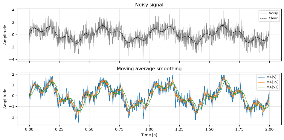
This is a causal FIR filter with uniform coefficients $h[k] = 1/N$. Its frequency response is a sinc-like shape with the first null at $f_s / N$. The moving average is optimal for reducing random white noise while preserving a sharp step response, but it is a poor lowpass filter in the frequency-domain sense, with only 13 dB of sidelobe rejection regardless of $N$.

import numpy as np
import matplotlib.pyplot as plt
from scipy import signal as sig

# Noisy test signal: slow sine + noise
rng = np.random.default_rng(42)
fs = 1000
t = np.arange(2000) / fs
x_clean = np.sin(2 * np.pi * 2 * t) + 0.5 * np.sin(2 * np.pi * 7 * t)
x = x_clean + 0.8 * rng.standard_normal(len(t))

fig, axes = plt.subplots(2, 1, figsize=(10, 5), sharex=True)
axes[0].plot(t, x, 'C7', linewidth=0.5, label='Noisy')
axes[0].plot(t, x_clean, 'k--', linewidth=1, label='Clean')
axes[0].legend(fontsize=8)
axes[0].set_ylabel('Amplitude')
axes[0].set_title('Noisy signal')

for N in [5, 15, 51]:
    h = np.ones(N) / N
    y = np.convolve(x, h, mode='full')[:len(x)]   # causal MA: shows the (N-1)/2 lag
    axes[1].plot(t, y, linewidth=1, label=f'MA({N})')

axes[1].plot(t, x_clean, 'k--', linewidth=1, alpha=0.5)
axes[1].set_xlabel('Time [s]')
axes[1].set_ylabel('Amplitude')
axes[1].set_title('Moving average smoothing')
axes[1].legend(fontsize=8)
for ax in axes:
    ax.grid(True, alpha=0.3)
fig.tight_layout()
plt.show()

Figure 1: Moving average smoothing: a 51-point MA filter removes high-frequency noise from a noisy sinusoid.

Longer windows remove more noise but also attenuate signal components and introduce lag. For the causal moving average, the group delay is $(N-1)/2$ samples.

Direct vs recursive implementation

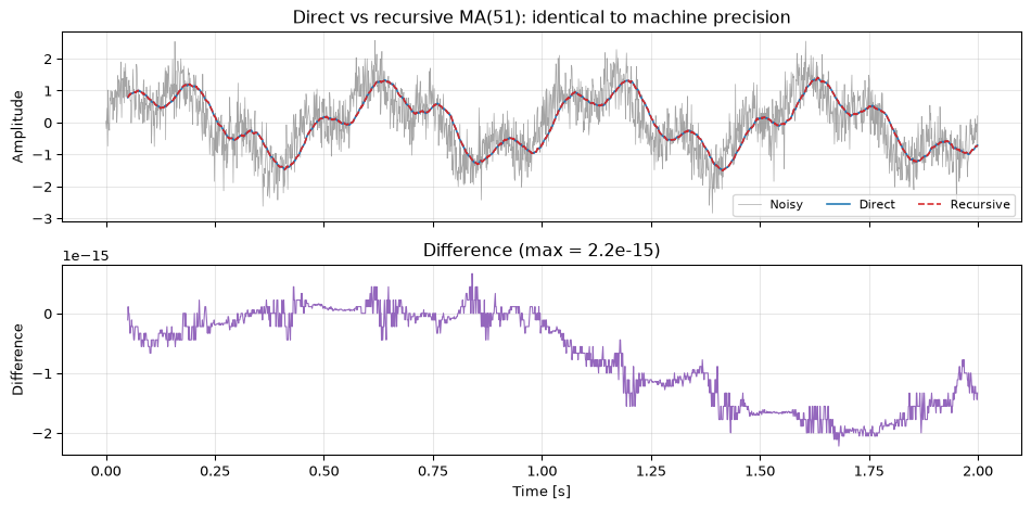
The direct form computes the full sum of $N$ samples for every output sample, costing $N-1$ additions and one division per output. For large $N$ this is wasteful, because consecutive windows share $N-1$ samples. The recursive (running-sum) form exploits that overlap:

\[s[n] = s[n-1] + x[n] - x[n-M]\] \[y[n] = s[n] / M\]

where $s[n]$ is the unscaled running sum. The output $y[n] = s[n]/M$ is identical to the direct form, but the update costs only one addition and one subtraction per sample regardless of $M$. The division by $M$ happens at the output and is not accumulated in the running sum, so the only rounding error source is the final division, not a per-step accumulation.

Structured this way, the moving average is a cascade of two sections:

\[H(z) = \frac{1}{M} \cdot \underbrace{\vphantom{\frac{1}{1}}\left(1 - z^{-M}\right)}_{\text{feedforward, delay }M} \cdot \underbrace{\frac{1}{1 - z^{-1}}}_{\text{feedback, delay }1}\]

The feedforward section (the comb) subtracts the sample that fell out of the window. The feedback section (the integrator) accumulates the result. The pole at $z=1$ is exactly canceled by the zero at $z=1$ in the numerator, which is why the overall filter is FIR despite the feedback path.

Figure 2: Cascade structure of the recursive moving average.

The diagram maps directly to hardware. The comb is a shift register of depth $M$ and a subtractor; the integrator is a single accumulator register and an adder. On an FPGA this costs $M$ flip-flops, one adder, and one subtractor (no multipliers). The embedded page walks through the VHDL.

What if we shift the pole?

The moving average places a pole exactly at $z=1$, canceled by a matching zero in the comb. If you shift that pole slightly inside the unit circle (replacing $\frac{1}{1-z^{-1}}$ with $\frac{1}{1-\alpha z^{-1}}$, $\alpha < 1$), the perfect cancellation breaks and the filter is no longer strictly FIR. The impulse response becomes an exponential envelope over $M$ samples followed by a decaying negative tail: $h[n] = \alpha^n$ for $0 \le n < M$, then $h[n] = -\alpha^{n-M}(1-\alpha^M)$ thereafter. But watch the DC gain: the comb’s zero at $z=1$ is untouched, so $H(1) = 0$ exactly, for any $\alpha < 1$. A constant input now decays to zero output with time constant $\approx 1/(1-\alpha)$ samples. What you have built is not an almost-moving-average: it is a DC blocker with a moving-average-shaped response above the corner at $f \approx (1-\alpha)f_s/2\pi$. That is a useful filter in its own right, but it is the opposite of a smoother whose job is to track a slowly varying level, so do not reach for a leaky pole to “stabilise” a moving average. The floating-point drift described below has better fixes; the embedded page works through them.

rng = np.random.default_rng(99)
M = 51
x_ma = x_clean + 0.5 * rng.standard_normal(len(t))

# Direct form: O(M) per sample
h = np.ones(M) / M
y_direct = np.convolve(x_ma, h, mode='full')[:len(x_ma)]

# Recursive form: O(1) per sample
s = np.sum(x_ma[:M])                      # seed the running sum with the first M samples
y_recursive = np.zeros(len(x_ma))
y_recursive[M-1] = s / M
for n in range(M, len(x_ma)):
    s += x_ma[n] - x_ma[n-M]              # one add, one sub (the whole update)
    y_recursive[n] = s / M

# The two forms produce identical output
max_diff = np.max(np.abs(y_direct[M-1:] - y_recursive[M-1:]))
assert max_diff < 3e-15, f"direct and recursive differ by {max_diff}"

fig, (ax1, ax2) = plt.subplots(2, 1, figsize=(10, 5), sharex=True)
ax1.plot(t, x_ma, 'C7', linewidth=0.5, alpha=0.7, label='Noisy')
ax1.plot(t[M-1:], y_direct[M-1:], 'C0', linewidth=1.2, label='Direct')
ax1.plot(t[M-1:], y_recursive[M-1:], 'C3', linewidth=1.2, linestyle='--', label='Recursive')
ax1.set_ylabel('Amplitude')
ax1.legend(fontsize=8, ncol=3)
ax1.grid(True, alpha=0.3)
ax2.plot(t[M-1:], y_direct[M-1:] - y_recursive[M-1:], 'C4', linewidth=0.8)
ax2.set_xlabel('Time [s]')
ax2.set_ylabel('Difference')
ax2.grid(True, alpha=0.3)
ax1.set_title(f'Direct vs recursive MA({M}): identical to machine precision')
ax2.set_title(f'Difference (max = {max_diff:.1e})')
fig.tight_layout()
plt.show()

Figure 3: Direct vs recursive moving average: identical output (difference < 1e-15), but the recursive form is O(1) per sample regardless of window length M.

The recursive moving average is a single-stage CIC filter with no decimation. The multirate chapter generalises this: an $N$-stage CIC decimating by $M$ is an $N$-stage moving average computed at the decimated rate, and the integrator-comb decomposition is exactly the recursive moving average structure. What the CIC adds is decimation (running the comb at a reduced rate) and cascading multiple stages for sharper stopband roll-off.

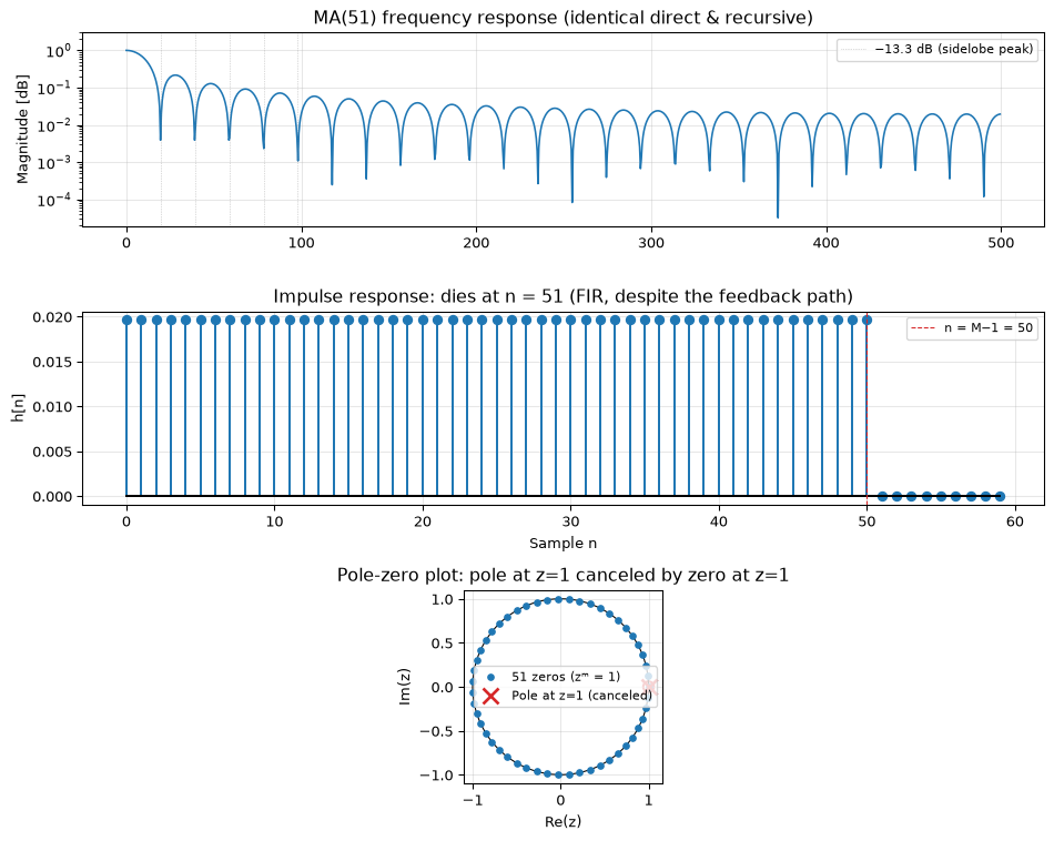
Even though the recursive form has a feedback path and looks like an IIR, the impulse response reveals the truth: the pole at $z=1$ is exactly canceled by a zero there, the response dies after exactly $M$ samples, and the frequency response is the characteristic sinc shape of the rectangular window.

# Generate the recursive form's impulse response by running the difference equation:
#   s[n] = s[n-1] + x[n] - x[n-M],   y[n] = s[n] / M
# with an impulse x[0] = 1, x[n>0] = 0.
imp = np.zeros(2048); imp[0] = 1.0
s_unscaled = 0
h_rec = np.zeros(2048)
for n in range(2048):
    xn_m = imp[n-M] if n >= M else 0.0
    s_unscaled += imp[n] - xn_m
    h_rec[n] = s_unscaled / M

# The recursive impulse response is FIR: zero after M samples (pole-zero cancellation at DC)
assert np.all(np.abs(h_rec[M:]) < 1e-15), \
    f"recursive impulse response is not FIR; samples beyond M={M} are nonzero"

# Direct FIR impulse response (zero-padded to same length for identical FFT grid)
h_dir = np.zeros(2048); h_dir[:M] = np.ones(M) / M
H_dir_fft = np.fft.rfft(h_dir)

# FFT of the recursive impulse response = its frequency response
H_rec_fft = np.fft.rfft(h_rec)
f_fft = np.fft.rfftfreq(2048, d=1/fs)

# Both on the same FFT grid (no interpolation needed)
freq_diff = np.max(np.abs(np.abs(H_rec_fft) - np.abs(H_dir_fft)))
assert freq_diff < 1e-15, f"direct and recursive frequency responses differ by {freq_diff}"

fig, (ax1, ax2, ax3) = plt.subplots(3, 1, figsize=(10, 8), sharex=False)

# Panel 1: frequency response
ax1.semilogy(f_fft[:1024], np.abs(H_rec_fft[:1024]), 'C0', linewidth=1.2)
for k in range(1, 6):
    null_hz = k * fs / M
    if null_hz < fs/2:
        ax1.axvline(null_hz, color='C7', linewidth=0.5, linestyle=':', alpha=0.6)
ax1.axhline(-13.3, color='C7', linewidth=0.5, linestyle=':', alpha=0.6, label='−13.3 dB (sidelobe peak)')
ax1.set_ylabel('Magnitude [dB]')
ax1.legend(fontsize=8)
ax1.grid(True, alpha=0.3)
ax1.set_title(f'MA({M}) frequency response (identical direct & recursive)')
ax1.set_ylim(-60, 3)

# Panel 2: impulse response (the pole-zero cancellation in action)
ax2.stem(np.arange(60), h_rec[:60], linefmt='C0-', markerfmt='C0o', basefmt='k-')
ax2.axvline(M-1, color='C3', linewidth=0.8, linestyle='--', label=f'n = M−1 = {M-1}')
ax2.set_xlabel('Sample n')
ax2.set_ylabel('h[n]')
ax2.legend(fontsize=8)
ax2.grid(True, alpha=0.3)
ax2.set_title(f'Impulse response: dies at n = {M} (FIR, despite the feedback path)')

# Panel 3: pole-zero plot
from matplotlib.patches import Circle
theta = np.linspace(0, 2*np.pi, 200)
ax3.plot(np.cos(theta), np.sin(theta), 'k-', linewidth=0.8)   # unit circle
# Zeros of 1 - z^-M: M equally spaced points on unit circle, including z=1
zeros = np.exp(2j * np.pi * np.arange(M) / M)
ax3.plot(zeros.real, zeros.imag, 'C0o', markersize=4, label=f'{M} zeros (zᵐ = 1)')
# Pole at z=1
ax3.plot(1, 0, 'C3x', markersize=10, markeredgewidth=2, label='Pole at z=1 (canceled)')
ax3.add_patch(Circle((1, 0), 0.06, fill=False, edgecolor='C3', linewidth=1.5))
ax3.set_xlabel('Re(z)')
ax3.set_ylabel('Im(z)')
ax3.set_aspect('equal')
ax3.legend(fontsize=8)
ax3.grid(True, alpha=0.3)
ax3.set_title('Pole-zero plot: pole at z=1 canceled by zero at z=1')
fig.tight_layout()
plt.show()

/tmp/ipykernel_2735/3919357287.py:41: UserWarning: Attempt to set non-positive ylim on a log-scaled axis will be ignored.
  ax1.set_ylim(-60, 3)

Figure 4: Frequency response of the moving average (M=51). The sinc-like shape has its first null at f_s/M and fixed −13.3 dB sidelobes regardless of window length. The recursive form’s impulse response, generated by running the feedback difference equation, is finite (M samples) and its FFT matches the direct FIR exactly.

The nulls at multiples of $f_s/M$ are the $M-1$ remaining zeros of $1 - z^{-M}$ that are not at DC. The −13.3 dB sidelobe peak is intrinsic to the rectangular window and does not improve with larger $M$; a longer window narrows the main lobe but leaves the sidelobe level unchanged. That is the fundamental limitation of the moving average as a lowpass filter, and why the filter design chapter spends so much time on window functions.

The Swiss Army knife of digital networks

Rick Lyons calls the integrator-comb pair the Swiss Army knife of digital networks (Lyons and Bell 2004), because the same two-building-block cascade yields half a dozen different DSP structures just by changing the tap point, the signs, and whether you decimate. The moving average ($M$-tap rectangular window) is the simplest member of this family. Connect the comb first and you get a differentiator ($M=1$) or a DC blocker ($\alpha$ in the integrator). Cascade $N$ stages and decimate by $M$ and you have a CIC filter, which we unpack in detail in the multirate chapter.

Floating-point drift in the running sum

The recursive form adds and subtracts values of similar magnitude from the same accumulator. In floating point, catastrophic cancellation can occur, and the running sum can slowly drift from the true sum over millions of samples. For long-running systems, periodically recompute the sum from scratch (once per second is ample at typical audio rates). In fixed-point with modular arithmetic the drift is not an issue because integer addition and subtraction wrap exactly, provided the accumulator is wide enough (see the embedded page for the bit-width requirement).

Savitzky-Golay filter

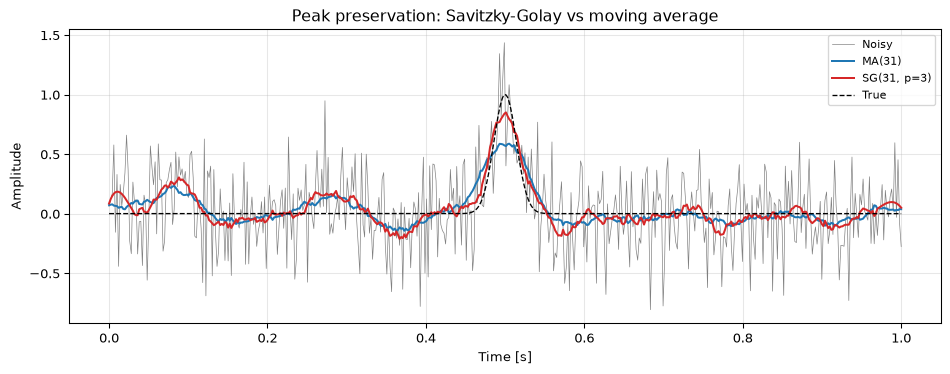
The Savitzky-Golay filter fits a local polynomial of degree $p$ to a window of $N$ points, then evaluates the polynomial at the centre of the window. Because a polynomial of degree $p$ passes through the filter unchanged, Savitzky-Golay preserves peaks, shoulders, and other features better than a moving average of the same length.

The filter coefficients are the result of a least-squares polynomial fit, computed once for given $N$ and $p$. SciPy provides savgol_filter with optional derivative computation, a useful side benefit, since the fitted polynomial can be differentiated analytically.

from scipy.signal import savgol_filter

# Signal with a sharp peak
t2 = np.linspace(0, 1, 500)
x_peak = np.exp(-((t2 - 0.5) / 0.02)**2) + 0.3 * rng.standard_normal(len(t2))

y_ma = np.convolve(x_peak, np.ones(31)/31, mode='same')
y_sg = savgol_filter(x_peak, window_length=31, polyorder=3)

fig, ax = plt.subplots(figsize=(10, 4))
ax.plot(t2, x_peak, 'C7', linewidth=0.5, label='Noisy')
ax.plot(t2, y_ma, 'C0', linewidth=1.5, label='MA(31)')
ax.plot(t2, y_sg, 'C3', linewidth=1.5, label='SG(31, p=3)')
ax.plot(t2, np.exp(-((t2 - 0.5) / 0.02)**2), 'k--', linewidth=1, label='True')
ax.set_xlabel('Time [s]')
ax.set_ylabel('Amplitude')
ax.legend(fontsize=8)
ax.grid(True, alpha=0.3)
ax.set_title('Peak preservation: Savitzky-Golay vs moving average')
fig.tight_layout()
plt.show()

Figure 5: Savitzky-Golay vs moving average on a signal with a sharp peak. The SG filter (polynomial order 3) preserves peak height and shape; the moving average flattens it.

Window length vs polynomial order

If $p$ is too close to $N-1$, the filter does almost no smoothing: it starts fitting the noise. A good starting point is $p = 2$ or $3$ with $N$ at least 3 to 5 times larger than $p + 1$. There is no universally optimal choice; it depends on the noise level and the features you want to preserve.

Exponential smoothing

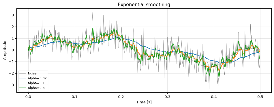
Exponential smoothing applies a first-order IIR filter:

\[y[n] = \alpha\, x[n] + (1 - \alpha)\, y[n-1], \quad 0 < \alpha \le 1\]

The smoothing factor $\alpha$ controls the trade-off: small $\alpha$ gives heavy smoothing (long memory), large $\alpha$ tracks the input closely. The impulse response decays geometrically: $h[n] = \alpha (1-\alpha)^n$, so recent samples contribute more than old ones.

The main advantage over moving averages is constant memory: only one state variable $y[n-1]$ is needed regardless of the effective smoothing window. This makes exponential smoothing popular in embedded systems and streaming applications.

fig, ax = plt.subplots(figsize=(10, 4))
ax.plot(t[:500], x[:500], 'C7', linewidth=0.5, label='Noisy')

for alpha in [0.02, 0.1, 0.3]:
    y_exp = np.zeros(500)
    y_exp[0] = x[0]
    for n in range(1, 500):
        y_exp[n] = alpha * x[n] + (1 - alpha) * y_exp[n-1]
    ax.plot(t[:500], y_exp, linewidth=1.5, label=f'alpha={alpha}')

ax.plot(t[:500], x_clean[:500], 'k--', linewidth=1, alpha=0.5)
ax.set_xlabel('Time [s]')
ax.set_ylabel('Amplitude')
ax.legend(fontsize=8)
ax.grid(True, alpha=0.3)
ax.set_title('Exponential smoothing')
fig.tight_layout()
plt.show()

Figure 6: Exponential smoothing with different values of alpha. Smaller alpha gives heavier smoothing but more lag.

The equivalent time constant is $\tau = -1 / \ln(1 - \alpha)$ samples. To relate $\alpha$ to a cutoff frequency: $\alpha = 1 - e^{-2\pi f_c / f_s}$.

Kernel smoothing

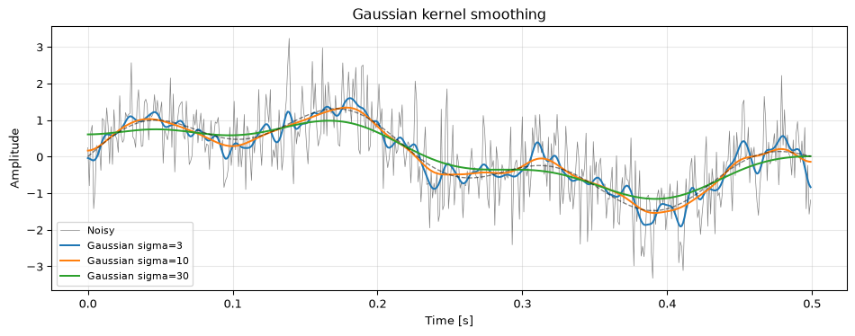
All the methods above are special cases of convolution with a kernel. Kernel smoothing generalises this by allowing any smooth, symmetric kernel: Gaussian, Epanechnikov, tricube, etc. The Gaussian kernel is the most common:

\[h[n] = \frac{1}{\sqrt{2\pi}\sigma} \exp\!\left(-\frac{n^2}{2\sigma^2}\right)\]

where $\sigma$ controls the bandwidth. Gaussian smoothing has the useful property that it never introduces new extrema (it only removes them) and its frequency response is also Gaussian: no sidelobes at all.

from scipy.ndimage import gaussian_filter1d

fig, ax = plt.subplots(figsize=(10, 4))
ax.plot(t[:500], x[:500], 'C7', linewidth=0.5, label='Noisy')

for sigma in [3, 10, 30]:
    y_gauss = gaussian_filter1d(x[:500], sigma=sigma)
    ax.plot(t[:500], y_gauss, linewidth=1.5, label=f'Gaussian sigma={sigma}')

ax.plot(t[:500], x_clean[:500], 'k--', linewidth=1, alpha=0.5)
ax.set_xlabel('Time [s]')
ax.set_ylabel('Amplitude')
ax.legend(fontsize=8)
ax.grid(True, alpha=0.3)
ax.set_title('Gaussian kernel smoothing')
fig.tight_layout()
plt.show()

Figure 7: Gaussian kernel smoothing at different bandwidths compared to a moving average of similar effective width.

When to use what

Method	Preserves peaks?	Constant memory?	Real-time?	Best for
Moving average	No	No ($N$ samples)	Yes	White noise on step-like signals
Savitzky-Golay	Yes	No ($N$ samples)	Yes	Preserving peak shape, derivatives
Exponential	No	Yes (1 sample)	Yes	Streaming, embedded systems
Gaussian kernel	No	No	Batch	Smooth, sidelobe-free suppression

The fundamental trade-off across all methods is smoothness vs lag. More aggressive smoothing removes more noise but delays features and can distort their shape. There is no way around this: it is a consequence of the uncertainty principle relating time and frequency resolution.

For real-time applications, exponential smoothing or short causal moving averages are the practical choices. For offline analysis where you can process the entire signal at once, Savitzky-Golay or Gaussian kernels usually give better results because they can be applied symmetrically (zero phase delay).

Tip

If you need smoothing without phase distortion, combine any of these methods with zero-phase filtering: apply the filter forward and backward.

Going further

Two questions every smoother runs into once you push it, and that the tidy table above quietly sidesteps.

Could the window adapt? A fixed window is always a compromise: too short in quiet stretches to knock down the noise, too long near a transient and it smears the sharp feature you cared about. Methods that vary the bandwidth with the local signal do exist, Stein’s unbiased risk estimate (SURE) and cross-validation among them, and they are theoretically appealing. They also add real complexity, which is why in practice most people pick a window length by eye and move on. Knowing the adaptive option is there matters more than reaching for it on day one.

What happens at the edges? Every finite-window smoother has a boundary problem: at the very start and end of the signal the full window is not available. Mirror padding, constant extrapolation, or shrinking the window are the usual fixes, and none is fully satisfactory, so results near the edges always deserve a second look. This is the same boundary headache you met in zero-phase filtering, and it never fully goes away.

References

Ballerini, M., N. Cabibbo, R. Candelier, A. Cavagna, E. Cisbani, I. Giardina, V. Lecomte, et al. 2008. “Interaction Ruling Animal Collective Behavior Depends on Topological Rather Than Metric Distance.” Proceedings of the National Academy of Sciences 105 (4): 1232–37.

Lyons, Richard G., and Amy E. Bell. 2004. “The Swiss Army Knife of Digital Networks.” IEEE Signal Processing Magazine 21 (3): 90–100.

Reynolds, Craig W. 1987. “Flocks, Herds and Schools: A Distributed Behavioral Model.” In Proceedings of the 14th Annual Conference on Computer Graphics and Interactive Techniques (SIGGRAPH), 25–34.

--- title: "Smoothing" subtitle: "Moving averages and beyond" aliases: - /topics/smoothing/index.html --- ::: {.callout-tip title="Nature's smoothing filter" appearance="simple"} A flock of starlings moves as one, thousands of birds producing smooth, coordinated motion from individually noisy heading decisions. Empirical studies show each bird tracks approximately 6-7 nearest neighbours [@ballerini2008interaction], averaging their directions, a spatial moving average that filters out individual jitter. Craig Reynolds formalised this as a computational model [@reynolds1987flocks], demonstrating that simple local averaging rules produce the complex collective patterns we observe. ::: Sensor data is noisy. Before you can extract meaningful features (peaks, trends, zero crossings) you typically need to smooth the signal. For embedded implementations (EMA and moving average with circular buffer on ESP32-S3 and STM32F4), see [Smoothing on Hardware](embedded.qmd). The question is never *whether* to smooth, but *how much* and *with what method*. Every smoothing technique trades off noise suppression against signal distortion, and the right choice depends on what you plan to do with the signal afterwards. We will work through four approaches: moving averages, Savitzky-Golay filters, exponential smoothing, and kernel smoothing. Each has a sweet spot and none is universally best, so the aim here is to build a feel for which one fits which job. ::: {.callout-note title="Prerequisites"} This topic assumes familiarity with [discrete-time systems](../02-discrete-time.qmd) (convolution, FIR filters) and [frequency-domain analysis](../05-frequency-domain.qmd). The moving average is introduced in [Chapter 2](../02-discrete-time.qmd) as a basic FIR filter. This page extends the idea. ::: <hr> ## Moving average The simplest smoother. An $N$-point moving average replaces each sample with the mean of its $N$ neighbours: $$y[n] = \frac{1}{N} \sum_{k=0}^{N-1} x[n-k]$$ This is a causal FIR filter with uniform coefficients $h[k] = 1/N$. Its frequency response is a sinc-like shape with the first null at $f_s / N$. The moving average is optimal for reducing random white noise while preserving a sharp step response, but it is a poor lowpass filter in the frequency-domain sense, with only 13 dB of sidelobe rejection regardless of $N$. ```{python} #| label: fig-smoothing-demo #| fig-cap: "Moving average smoothing: a 51-point MA filter removes high-frequency noise from a noisy sinusoid." import numpy as np import matplotlib.pyplot as plt from scipy import signal as sig # Noisy test signal: slow sine + noise rng = np.random.default_rng(42) fs = 1000 t = np.arange(2000) / fs x_clean = np.sin(2 * np.pi * 2 * t) + 0.5 * np.sin(2 * np.pi * 7 * t) x = x_clean + 0.8 * rng.standard_normal(len(t)) fig, axes = plt.subplots(2, 1, figsize=(10, 5), sharex=True) axes[0].plot(t, x, 'C7', linewidth=0.5, label='Noisy') axes[0].plot(t, x_clean, 'k--', linewidth=1, label='Clean') axes[0].legend(fontsize=8) axes[0].set_ylabel('Amplitude') axes[0].set_title('Noisy signal') for N in [5, 15, 51]: h = np.ones(N) / N y = np.convolve(x, h, mode='full')[:len(x)] # causal MA: shows the (N-1)/2 lag axes[1].plot(t, y, linewidth=1, label=f'MA({N})') axes[1].plot(t, x_clean, 'k--', linewidth=1, alpha=0.5) axes[1].set_xlabel('Time [s]') axes[1].set_ylabel('Amplitude') axes[1].set_title('Moving average smoothing') axes[1].legend(fontsize=8) for ax in axes: ax.grid(True, alpha=0.3) fig.tight_layout() plt.show() ``` Longer windows remove more noise but also attenuate signal components and introduce lag. For the causal moving average, the group delay is $(N-1)/2$ samples. ### Direct vs recursive implementation The direct form computes the full sum of $N$ samples for every output sample, costing $N-1$ additions and one division per output. For large $N$ this is wasteful, because consecutive windows share $N-1$ samples. The **recursive** (running-sum) form exploits that overlap: $$s[n] = s[n-1] + x[n] - x[n-M]$$ $$y[n] = s[n] / M$$ where $s[n]$ is the unscaled running sum. The output $y[n] = s[n]/M$ is identical to the direct form, but the update costs only **one addition and one subtraction** per sample regardless of $M$. The division by $M$ happens at the output and is not accumulated in the running sum, so the only rounding error source is the final division, not a per-step accumulation. Structured this way, the moving average is a cascade of two sections: $$H(z) = \frac{1}{M} \cdot \underbrace{\vphantom{\frac{1}{1}}\left(1 - z^{-M}\right)}_{\text{feedforward, delay }M} \cdot \underbrace{\frac{1}{1 - z^{-1}}}_{\text{feedback, delay }1}$$ The feedforward section (the **comb**) subtracts the sample that fell out of the window. The feedback section (the **integrator**) accumulates the result. The pole at $z=1$ is exactly canceled by the zero at $z=1$ in the numerator, which is why the overall filter is FIR despite the feedback path. ```{dot} //| label: fig-ma-cascade //| echo: false //| fig-cap: "Cascade structure of the recursive moving average." graph { layout=neato node [fontname="sans-serif" fontsize=12] edge [arrowsize=0.55 dir=forward] x [label="x[n]" shape=plaintext fontname="serif"] br [label="" shape=point width=0.05] zm [label="z^-M" shape=box width=0.62 height=0.40] add [label="+" shape=circle width=0.32 fixedsize=true] z1 [label="z^-1" shape=box width=0.52 height=0.40] gm [label="1/M" shape=invtriangle orientation=270 width=0.62 height=0.52 fixedsize=true] y [label="y[n]" shape=plaintext fontname="serif"] x -- br br -- add br -- zm zm -- add [headlabel="- "] add -- z1 z1 -- gm gm -- y z1 -- add [style=dashed] } ``` The diagram maps directly to hardware. The comb is a shift register of depth $M$ and a subtractor; the integrator is a single accumulator register and an adder. On an FPGA this costs $M$ flip-flops, one adder, and one subtractor (no multipliers). The [embedded page](embedded.qmd) walks through the VHDL. ::: {.callout-tip title="What if we shift the pole?"} The moving average places a pole exactly at $z=1$, canceled by a matching zero in the comb. If you shift that pole slightly inside the unit circle (replacing $\frac{1}{1-z^{-1}}$ with $\frac{1}{1-\alpha z^{-1}}$, $\alpha < 1$), the perfect cancellation breaks and the filter is no longer strictly FIR. The impulse response becomes an exponential envelope over $M$ samples followed by a decaying negative tail: $h[n] = \alpha^n$ for $0 \le n < M$, then $h[n] = -\alpha^{n-M}(1-\alpha^M)$ thereafter. But watch the DC gain: the comb's zero at $z=1$ is untouched, so $H(1) = 0$ *exactly*, for any $\alpha < 1$. A constant input now decays to zero output with time constant $\approx 1/(1-\alpha)$ samples. What you have built is not an almost-moving-average: it is a **DC blocker** with a moving-average-shaped response above the corner at $f \approx (1-\alpha)f_s/2\pi$. That is a useful filter in its own right, but it is the opposite of a smoother whose job is to track a slowly varying level, so do not reach for a leaky pole to "stabilise" a moving average. The floating-point drift described below has better fixes; the [embedded page](embedded.qmd) works through them. ::: ```{python} #| label: fig-ma-recursive #| fig-cap: "Direct vs recursive moving average: identical output (difference < 1e-15), but the recursive form is O(1) per sample regardless of window length M." rng = np.random.default_rng(99) M = 51 x_ma = x_clean + 0.5 * rng.standard_normal(len(t)) # Direct form: O(M) per sample h = np.ones(M) / M y_direct = np.convolve(x_ma, h, mode='full')[:len(x_ma)] # Recursive form: O(1) per sample s = np.sum(x_ma[:M]) # seed the running sum with the first M samples y_recursive = np.zeros(len(x_ma)) y_recursive[M-1] = s / M for n in range(M, len(x_ma)): s += x_ma[n] - x_ma[n-M] # one add, one sub (the whole update) y_recursive[n] = s / M # The two forms produce identical output max_diff = np.max(np.abs(y_direct[M-1:] - y_recursive[M-1:])) assert max_diff < 3e-15, f"direct and recursive differ by {max_diff}" fig, (ax1, ax2) = plt.subplots(2, 1, figsize=(10, 5), sharex=True) ax1.plot(t, x_ma, 'C7', linewidth=0.5, alpha=0.7, label='Noisy') ax1.plot(t[M-1:], y_direct[M-1:], 'C0', linewidth=1.2, label='Direct') ax1.plot(t[M-1:], y_recursive[M-1:], 'C3', linewidth=1.2, linestyle='--', label='Recursive') ax1.set_ylabel('Amplitude') ax1.legend(fontsize=8, ncol=3) ax1.grid(True, alpha=0.3) ax2.plot(t[M-1:], y_direct[M-1:] - y_recursive[M-1:], 'C4', linewidth=0.8) ax2.set_xlabel('Time [s]') ax2.set_ylabel('Difference') ax2.grid(True, alpha=0.3) ax1.set_title(f'Direct vs recursive MA({M}): identical to machine precision') ax2.set_title(f'Difference (max = {max_diff:.1e})') fig.tight_layout() plt.show() ``` The recursive moving average is a **single-stage CIC filter** with no decimation. The [multirate chapter](../10-multirate/index.qmd) generalises this: an $N$-stage CIC decimating by $M$ is an $N$-stage moving average computed at the decimated rate, and the integrator-comb decomposition is exactly the recursive moving average structure. What the CIC adds is decimation (running the comb at a reduced rate) and cascading multiple stages for sharper stopband roll-off. Even though the recursive form has a feedback path and looks like an IIR, the impulse response reveals the truth: the pole at $z=1$ is exactly canceled by a zero there, the response dies after exactly $M$ samples, and the frequency response is the characteristic sinc shape of the rectangular window. ```{python} #| label: fig-ma-frequency #| fig-cap: "Frequency response of the moving average (M=51). The sinc-like shape has its first null at f_s/M and fixed −13.3 dB sidelobes regardless of window length. The recursive form's impulse response, generated by running the feedback difference equation, is finite (M samples) and its FFT matches the direct FIR exactly." # Generate the recursive form's impulse response by running the difference equation: # s[n] = s[n-1] + x[n] - x[n-M], y[n] = s[n] / M # with an impulse x[0] = 1, x[n>0] = 0. imp = np.zeros(2048); imp[0] = 1.0 s_unscaled = 0 h_rec = np.zeros(2048) for n in range(2048): xn_m = imp[n-M] if n >= M else 0.0 s_unscaled += imp[n] - xn_m h_rec[n] = s_unscaled / M # The recursive impulse response is FIR: zero after M samples (pole-zero cancellation at DC) assert np.all(np.abs(h_rec[M:]) < 1e-15), \ f"recursive impulse response is not FIR; samples beyond M={M} are nonzero" # Direct FIR impulse response (zero-padded to same length for identical FFT grid) h_dir = np.zeros(2048); h_dir[:M] = np.ones(M) / M H_dir_fft = np.fft.rfft(h_dir) # FFT of the recursive impulse response = its frequency response H_rec_fft = np.fft.rfft(h_rec) f_fft = np.fft.rfftfreq(2048, d=1/fs) # Both on the same FFT grid (no interpolation needed) freq_diff = np.max(np.abs(np.abs(H_rec_fft) - np.abs(H_dir_fft))) assert freq_diff < 1e-15, f"direct and recursive frequency responses differ by {freq_diff}" fig, (ax1, ax2, ax3) = plt.subplots(3, 1, figsize=(10, 8), sharex=False) # Panel 1: frequency response ax1.semilogy(f_fft[:1024], np.abs(H_rec_fft[:1024]), 'C0', linewidth=1.2) for k in range(1, 6): null_hz = k * fs / M if null_hz < fs/2: ax1.axvline(null_hz, color='C7', linewidth=0.5, linestyle=':', alpha=0.6) ax1.axhline(-13.3, color='C7', linewidth=0.5, linestyle=':', alpha=0.6, label='−13.3 dB (sidelobe peak)') ax1.set_ylabel('Magnitude [dB]') ax1.legend(fontsize=8) ax1.grid(True, alpha=0.3) ax1.set_title(f'MA({M}) frequency response (identical direct & recursive)') ax1.set_ylim(-60, 3) # Panel 2: impulse response (the pole-zero cancellation in action) ax2.stem(np.arange(60), h_rec[:60], linefmt='C0-', markerfmt='C0o', basefmt='k-') ax2.axvline(M-1, color='C3', linewidth=0.8, linestyle='--', label=f'n = M−1 = {M-1}') ax2.set_xlabel('Sample n') ax2.set_ylabel('h[n]') ax2.legend(fontsize=8) ax2.grid(True, alpha=0.3) ax2.set_title(f'Impulse response: dies at n = {M} (FIR, despite the feedback path)') # Panel 3: pole-zero plot from matplotlib.patches import Circle theta = np.linspace(0, 2*np.pi, 200) ax3.plot(np.cos(theta), np.sin(theta), 'k-', linewidth=0.8) # unit circle # Zeros of 1 - z^-M: M equally spaced points on unit circle, including z=1 zeros = np.exp(2j * np.pi * np.arange(M) / M) ax3.plot(zeros.real, zeros.imag, 'C0o', markersize=4, label=f'{M} zeros (zᵐ = 1)') # Pole at z=1 ax3.plot(1, 0, 'C3x', markersize=10, markeredgewidth=2, label='Pole at z=1 (canceled)') ax3.add_patch(Circle((1, 0), 0.06, fill=False, edgecolor='C3', linewidth=1.5)) ax3.set_xlabel('Re(z)') ax3.set_ylabel('Im(z)') ax3.set_aspect('equal') ax3.legend(fontsize=8) ax3.grid(True, alpha=0.3) ax3.set_title('Pole-zero plot: pole at z=1 canceled by zero at z=1') fig.tight_layout() plt.show() ``` The nulls at multiples of $f_s/M$ are the $M-1$ remaining zeros of $1 - z^{-M}$ that are not at DC. The −13.3 dB sidelobe peak is intrinsic to the rectangular window and does not improve with larger $M$; a longer window narrows the main lobe but leaves the sidelobe *level* unchanged. That is the fundamental limitation of the moving average as a lowpass filter, and why the [filter design chapter](../06-filter-design.qmd) spends so much time on window functions. ::: {.callout-tip title="The Swiss Army knife of digital networks"} Rick Lyons calls the integrator-comb pair the Swiss Army knife of digital networks [@lyons2004swissarmy], because the same two-building-block cascade yields half a dozen different DSP structures just by changing the tap point, the signs, and whether you decimate. The moving average ($M$-tap rectangular window) is the simplest member of this family. Connect the comb first and you get a differentiator ($M=1$) or a DC blocker ($\alpha$ in the integrator). Cascade $N$ stages and decimate by $M$ and you have a CIC filter, which we unpack in detail in the [multirate chapter](../10-multirate/index.qmd). ::: ::: {.callout-warning title="Floating-point drift in the running sum"} The recursive form adds and subtracts values of similar magnitude from the same accumulator. In floating point, catastrophic cancellation can occur, and the running sum can slowly drift from the true sum over millions of samples. For long-running systems, periodically recompute the sum from scratch (once per second is ample at typical audio rates). In fixed-point with modular arithmetic the drift is not an issue because integer addition and subtraction wrap exactly, provided the accumulator is wide enough (see the [embedded page](embedded.qmd) for the bit-width requirement). ::: <hr> ## Savitzky-Golay filter The Savitzky-Golay filter fits a local polynomial of degree $p$ to a window of $N$ points, then evaluates the polynomial at the centre of the window. Because a polynomial of degree $p$ passes through the filter unchanged, Savitzky-Golay preserves peaks, shoulders, and other features better than a moving average of the same length. The filter coefficients are the result of a least-squares polynomial fit, computed once for given $N$ and $p$. SciPy provides `savgol_filter` with optional derivative computation, a useful side benefit, since the fitted polynomial can be differentiated analytically. ```{python} #| label: fig-savgol #| fig-cap: "Savitzky-Golay vs moving average on a signal with a sharp peak. The SG filter (polynomial order 3) preserves peak height and shape; the moving average flattens it." from scipy.signal import savgol_filter # Signal with a sharp peak t2 = np.linspace(0, 1, 500) x_peak = np.exp(-((t2 - 0.5) / 0.02)**2) + 0.3 * rng.standard_normal(len(t2)) y_ma = np.convolve(x_peak, np.ones(31)/31, mode='same') y_sg = savgol_filter(x_peak, window_length=31, polyorder=3) fig, ax = plt.subplots(figsize=(10, 4)) ax.plot(t2, x_peak, 'C7', linewidth=0.5, label='Noisy') ax.plot(t2, y_ma, 'C0', linewidth=1.5, label='MA(31)') ax.plot(t2, y_sg, 'C3', linewidth=1.5, label='SG(31, p=3)') ax.plot(t2, np.exp(-((t2 - 0.5) / 0.02)**2), 'k--', linewidth=1, label='True') ax.set_xlabel('Time [s]') ax.set_ylabel('Amplitude') ax.legend(fontsize=8) ax.grid(True, alpha=0.3) ax.set_title('Peak preservation: Savitzky-Golay vs moving average') fig.tight_layout() plt.show() ``` ::: {.callout-warning title="Window length vs polynomial order"} If $p$ is too close to $N-1$, the filter does almost no smoothing: it starts fitting the noise. A good starting point is $p = 2$ or $3$ with $N$ at least 3 to 5 times larger than $p + 1$. There is no universally optimal choice; it depends on the noise level and the features you want to preserve. ::: <hr> ## Exponential smoothing Exponential smoothing applies a first-order IIR filter: $$y[n] = \alpha\, x[n] + (1 - \alpha)\, y[n-1], \quad 0 < \alpha \le 1$$ The smoothing factor $\alpha$ controls the trade-off: small $\alpha$ gives heavy smoothing (long memory), large $\alpha$ tracks the input closely. The impulse response decays geometrically: $h[n] = \alpha (1-\alpha)^n$, so recent samples contribute more than old ones. The main advantage over moving averages is **constant memory**: only one state variable $y[n-1]$ is needed regardless of the effective smoothing window. This makes exponential smoothing popular in embedded systems and streaming applications. ```{python} #| label: fig-exponential #| fig-cap: "Exponential smoothing with different values of alpha. Smaller alpha gives heavier smoothing but more lag." fig, ax = plt.subplots(figsize=(10, 4)) ax.plot(t[:500], x[:500], 'C7', linewidth=0.5, label='Noisy') for alpha in [0.02, 0.1, 0.3]: y_exp = np.zeros(500) y_exp[0] = x[0] for n in range(1, 500): y_exp[n] = alpha * x[n] + (1 - alpha) * y_exp[n-1] ax.plot(t[:500], y_exp, linewidth=1.5, label=f'alpha={alpha}') ax.plot(t[:500], x_clean[:500], 'k--', linewidth=1, alpha=0.5) ax.set_xlabel('Time [s]') ax.set_ylabel('Amplitude') ax.legend(fontsize=8) ax.grid(True, alpha=0.3) ax.set_title('Exponential smoothing') fig.tight_layout() plt.show() ``` The equivalent time constant is $\tau = -1 / \ln(1 - \alpha)$ samples. To relate $\alpha$ to a cutoff frequency: $\alpha = 1 - e^{-2\pi f_c / f_s}$. <hr> ## Kernel smoothing All the methods above are special cases of convolution with a kernel. **Kernel smoothing** generalises this by allowing any smooth, symmetric kernel: Gaussian, Epanechnikov, tricube, etc. The Gaussian kernel is the most common: $$h[n] = \frac{1}{\sqrt{2\pi}\sigma} \exp\!\left(-\frac{n^2}{2\sigma^2}\right)$$ where $\sigma$ controls the bandwidth. Gaussian smoothing has the useful property that it never introduces new extrema (it only removes them) and its frequency response is also Gaussian: no sidelobes at all. ```{python} #| label: fig-kernel #| fig-cap: "Gaussian kernel smoothing at different bandwidths compared to a moving average of similar effective width." from scipy.ndimage import gaussian_filter1d fig, ax = plt.subplots(figsize=(10, 4)) ax.plot(t[:500], x[:500], 'C7', linewidth=0.5, label='Noisy') for sigma in [3, 10, 30]: y_gauss = gaussian_filter1d(x[:500], sigma=sigma) ax.plot(t[:500], y_gauss, linewidth=1.5, label=f'Gaussian sigma={sigma}') ax.plot(t[:500], x_clean[:500], 'k--', linewidth=1, alpha=0.5) ax.set_xlabel('Time [s]') ax.set_ylabel('Amplitude') ax.legend(fontsize=8) ax.grid(True, alpha=0.3) ax.set_title('Gaussian kernel smoothing') fig.tight_layout() plt.show() ``` <hr> ## When to use what | Method | Preserves peaks? | Constant memory? | Real-time? | Best for | |--------|:-:|:-:|:-:|------| | Moving average | No | No ($N$ samples) | Yes | White noise on step-like signals | | Savitzky-Golay | Yes | No ($N$ samples) | Yes | Preserving peak shape, derivatives | | Exponential | No | Yes (1 sample) | Yes | Streaming, embedded systems | | Gaussian kernel | No | No | Batch | Smooth, sidelobe-free suppression | The fundamental trade-off across all methods is **smoothness vs lag**. More aggressive smoothing removes more noise but delays features and can distort their shape. There is no way around this: it is a consequence of the uncertainty principle relating time and frequency resolution. For real-time applications, exponential smoothing or short causal moving averages are the practical choices. For offline analysis where you can process the entire signal at once, Savitzky-Golay or Gaussian kernels usually give better results because they can be applied symmetrically (zero phase delay). ::: {.callout-tip} If you need smoothing without phase distortion, combine any of these methods with [zero-phase filtering](../zero-phase.qmd): apply the filter forward and backward. ::: <hr> ## Going further Two questions every smoother runs into once you push it, and that the tidy table above quietly sidesteps. **Could the window adapt?** A fixed window is always a compromise: too short in quiet stretches to knock down the noise, too long near a transient and it smears the sharp feature you cared about. Methods that vary the bandwidth with the local signal do exist, Stein's unbiased risk estimate (SURE) and cross-validation among them, and they are theoretically appealing. They also add real complexity, which is why in practice most people pick a window length by eye and move on. Knowing the adaptive option is there matters more than reaching for it on day one. **What happens at the edges?** Every finite-window smoother has a boundary problem: at the very start and end of the signal the full window is not available. Mirror padding, constant extrapolation, or shrinking the window are the usual fixes, and none is fully satisfactory, so results near the edges always deserve a second look. This is the same boundary headache you met in [zero-phase filtering](../zero-phase.qmd), and it never fully goes away. ## References ::: {#refs} :::