On paper a digital filter has infinite precision: its coefficients are real numbers and its arithmetic is exact. On a microcontroller it does not. Coefficients land on a finite grid, every multiply has to be rounded back to the register width, and sums can overflow. These are the finite word-length effects, and they are where a design that looks perfect in double precision can degrade, distort, or even go unstable once it meets the metal.
This page is the theory companion to the practical fixed-point code in the biquad embedded page. It first sets out how fixed-point numbers are represented, then collects the four things that bite, says how big each one is, and shows the structural choices that tame them. The recurring lesson is the same one that motivates cascaded second-order sections: second-order sections are not a stylistic preference, they are what keeps a fixed-point filter alive.
There are really only a handful of distinct effects:
Quantization noise from representing signals and coefficients on a grid.
Coefficient sensitivity: the grid moves the poles and zeros, sometimes catastrophically.
Round-off noise from rounding every intermediate product.
Overflow and the limit cycles that nonlinearity can sustain.
We take them one at a time. The reference throughout is Manolakis and Ingle (Manolakis and Ingle 2011, ch. 15).
Prerequisites
The z-domain for poles, zeros, and what moving a pole towards the unit circle does to stability; filter design and filter structures for direct forms and second-order sections, which is the choice this page turns into an arithmetic argument. Biquad filters and its embedded page are the practical companion: that page writes the fixed-point code, this one says why it is shaped the way it is. The overflow section near the end works in state space; model-based filtering sets that up if it is unfamiliar.
Round a signal to a grid of step \(\Delta\) and you make an error of at most \(\Delta/2\). Model that error as a uniform random variable on \([-\Delta/2, \Delta/2]\) and it has variance
\[\sigma_e^2 = \frac{\Delta^2}{12}.\]
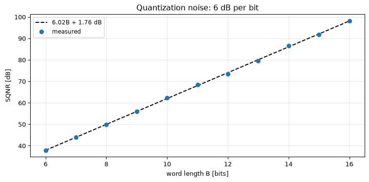
For a \(B\)-bit converter spanning the signal range, \(\Delta\) halves with every extra bit, so the noise power drops by a factor of four. Against a full-scale sinusoid this gives the headline rule of thumb for the signal-to-quantization-noise ratio,
about 6 dB, or one bit, of dynamic range per bit of word length. The demo quantizes a full-scale sine to a range of word lengths and compares the measured SQNR to the formula.
Show the code
n = np.arange(40000)sine =0.99* np.sin(2* np.pi * n /200) # near-full-scale, no overload from 6 bits upbits = np.arange(6, 17)measured = np.array([sqnr_db(sine, quantize(sine, b)) for b in bits])theory = theoretical_sqnr_db(bits)assert np.max(np.abs(measured - theory)) <1.0# within 1 dB across the sweepfig, ax = plt.subplots(figsize=(8, 4))ax.plot(bits, theory, 'k--', label='6.02B + 1.76 dB')ax.plot(bits, measured, 'o', color='C0', label='measured')ax.set_xlabel('word length B [bits]'); ax.set_ylabel('SQNR [dB]')ax.set_title('Quantization noise: 6 dB per bit')ax.legend(fontsize=9); ax.grid(True, alpha=0.3)fig.tight_layout()plt.show()
Figure 1: Measured signal-to-quantization-noise ratio of a full-scale sinusoid versus word length, against the 6.02B + 1.76 dB rule. The match is within a fraction of a dB.
This is the budget you start from: a 12-bit ADC gives you about 74 dB to work with, a 16-bit one about 98 dB. Everything below eats into it.
Fixed-point representation: Q-formats
When the target has no floating-point unit (a Cortex-M0+, an AVR) or when power and throughput demand the integer path, signals and coefficients are stored as scaled integers in Q-format. A Q\(m\).\(n\) number is a two’s-complement integer read as having \(n\) fractional bits; the two common audio choices both represent a value in \([-1, 1)\):
Format
Bits
Range
Resolution
Use case
Q15
16
\([-1,\ 1 - 2^{-15})\)
\(3.05 \times 10^{-5}\)
Low-power, small filters
Q31
32
\([-1,\ 1 - 2^{-31})\)
\(4.66 \times 10^{-10}\)
High-quality audio
A coefficient stored in Q15 is an integer in \([-32768, 32767]\) standing for \(\text{integer}/32768\), and all arithmetic stays in the integer domain. The programmer’s job is to track where the binary point lands after each operation: a Q15 times Q15 product is Q30 (it has 30 fractional bits in 32), so it must be shifted back before it is stored or summed. Coefficients that exceed \(\pm 1\) (a high-gain peaking EQ, for instance) do not fit Q15 at all and must be pre-scaled, with a compensating gain applied elsewhere. This bookkeeping is the price of dropping the FPU, and it is why the biquad embedded page leans on CMSIS-DSP’s ready-made Q15 and Q31 filters rather than rolling the arithmetic by hand.
Coefficient quantization: the poles move
Quantizing the signal adds noise. Quantizing the coefficients does something more dangerous: it changes the filter. Each coefficient is forced onto the grid,
and those perturbations move the poles and zeros. A sensitivity analysis (Manolakis and Ingle 2011, eq. 15.70) shows that the shift of pole \(p_i\) depends on \(1/\prod_{j\neq i}(p_i - p_j)\): when poles are tightly clustered, as they are in a narrowband or high-order filter, that denominator is tiny and the poles are exquisitely sensitive. Implement such a filter as one high-order direct-form transfer function and quantization can fling a pole clean outside the unit circle.
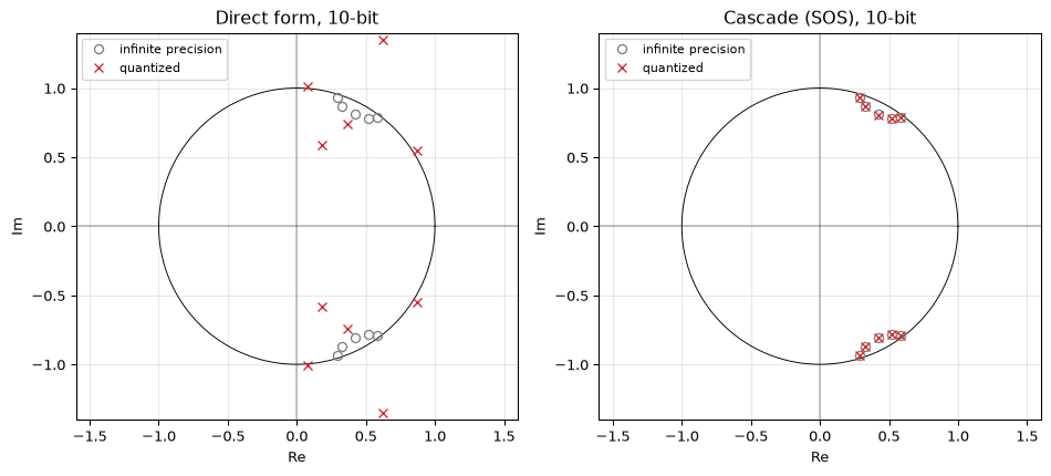
The cure is structural. Split the filter into second-order sections: each section holds one conjugate pole pair, its two coefficients stay in \([-2, 2]\), and the pole of one section no longer depends on the coefficients of the others. The demo takes a 5th-order elliptic bandpass and quantizes its coefficients two ways.
Show the code
order, wn = signal.ellipord([0.3, 0.4], [0.2, 0.5], 0.1, 60)b, a = signal.ellip(order, 0.1, 60, wn, btype='band')sos = signal.ellip(order, 0.1, 60, wn, btype='band', output='sos')n_bits =10c_max =2** np.ceil(np.log2(np.max(np.abs(a)) +1.0)) # direct form needs many integer bitsa_q = quantize_coeffs(np.asarray(a), n_bits, c_max=c_max)b_q = quantize_coeffs(np.asarray(b), n_bits, c_max=c_max)sos_q = np.array([quantize_coeffs(s, n_bits, c_max=2.0) for s in sos])# The whole point, checked at render time:assert is_stable(a) andnot is_stable(a_q) and sos_is_stable(sos_q)print(f"direct form needs c_max = {c_max:.0f} (|a| up to {np.max(np.abs(a)):.1f}); "f"quantized direct form stable? {is_stable(a_q)}; quantized SOS stable? {sos_is_stable(sos_q)}")def poles_ba(a):return np.roots(a)def poles_sos(sos):return np.concatenate([np.roots(s[3:6]) for s in np.atleast_2d(sos)])fig, axes = plt.subplots(1, 2, figsize=(10, 5))theta = np.linspace(0, 2* np.pi, 400)for ax, p_inf, p_q, title in [ (axes[0], poles_ba(a), poles_ba(a_q), f'Direct form, {n_bits}-bit'), (axes[1], poles_sos(sos), poles_sos(sos_q), f'Cascade (SOS), {n_bits}-bit')]: ax.plot(np.cos(theta), np.sin(theta), 'k-', linewidth=0.7) ax.plot(p_inf.real, p_inf.imag, 'o', mfc='none', mec='C7', label='infinite precision') ax.plot(p_q.real, p_q.imag, 'x', color='C3', label='quantized') ax.set_title(title); ax.set_xlabel('Re'); ax.set_ylabel('Im') ax.set_aspect('equal'); ax.set_xlim(-1.6, 1.6); ax.set_ylim(-1.4, 1.4) ax.axhline(0, color='k', lw=0.3); ax.axvline(0, color='k', lw=0.3) ax.grid(True, alpha=0.3); ax.legend(fontsize=8, loc='upper left')fig.tight_layout()plt.show()
direct form needs c_max = 64 (|a| up to 32.0); quantized direct form stable? False; quantized SOS stable? True
Figure 2: A 5th-order elliptic bandpass under 10-bit coefficient quantization. As one direct-form (b, a) transfer function (left) three of its conjugate pole pairs are pushed outside the unit circle and the filter is unstable. As cascaded second-order sections (right) the same word length leaves every pole in place.
The direct form fails not only because its poles are clustered but because its coefficients have a huge dynamic range (the denominator coefficients of a 10th-degree polynomial run into the tens), so at a fixed word length the grid spacing on them is coarse. The cascade form keeps every coefficient small and every pole independent. This is the numerical argument behind the biquad chapter, made quantitative.
Round-off noise and the accumulator
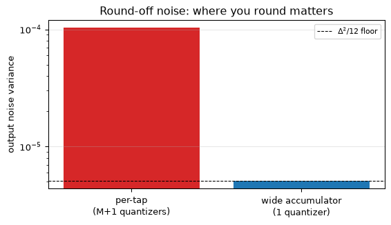
Even with the poles safely placed, every multiply inside the filter produces a full-width product that has to be rounded back to the register, and each rounding injects a fresh \(\Delta^2/12\) of noise. For a length-\((M{+}1)\) FIR filter that rounds after every tap, the noise powers add and the output noise variance is
\[\sigma_g^2 = (M+1)\,\frac{\Delta^2}{12},\]
so a longer filter is a noisier one. The fix is the double-width accumulator: keep the running sum at full precision and round only once, at the very end. Then a single quantizer contributes and the output noise collapses to
\[\sigma_g^2 = \frac{\Delta^2}{12},\]
independent of filter length. This is exactly why DSP cores carry a wide accumulator: a \(B\)-bit by \(B\)-bit product is about \(2B\) bits, so the running sum is kept at double width plus a few guard bits, and often much wider (CMSIS-DSP’s Q15 biquads accumulate in 64 bits). The same point is made in passing on the biquad embedded page and quantified here.
Show the code
rng = np.random.default_rng(0)M1 =33# number of tapsh = signal.firwin(M1, 0.25)B =8delta = quantization_step(B)x = (2* rng.random(20000) -1) *0.9# full-ish scale random inputexact = np.convolve(x, h) # full, infinite-precision reference# round after every tap: M+1 quantizers, summed in one aligned frameper_tap = np.zeros(len(exact))for k inrange(M1): contrib = np.zeros(len(exact)) contrib[k:k +len(x)] = h[k] * x per_tap += quantize(contrib, B)single = quantize(exact, B) # wide accumulator: sum exactly, round onceinterior =slice(M1, len(x)) # region where all taps are activevar_per_tap = np.var((per_tap - exact)[interior])var_single = np.var((single - exact)[interior])pred_single = delta**2/12assert0.5< var_single / pred_single <2.0# single quantizer hits the floorassert var_per_tap >8* var_single # per-tap is far noisierprint(f"single-quantizer noise var {var_single:.2e} (Delta^2/12 = {pred_single:.2e})")print(f"per-tap noise var {var_per_tap:.2e}")print(f"wide accumulator is {var_per_tap / var_single:.0f}x quieter for {M1} taps")fig, ax = plt.subplots(figsize=(6, 3.5))ax.bar(['per-tap\n(M+1 quantizers)', 'wide accumulator\n(1 quantizer)'], [var_per_tap, var_single], color=['C3', 'C0'])ax.axhline(pred_single, color='k', linestyle='--', linewidth=0.8, label=r'$\Delta^2/12$ floor')ax.set_yscale('log'); ax.set_ylabel('output noise variance')ax.set_title('Round-off noise: where you round matters')ax.legend(fontsize=8); ax.grid(True, alpha=0.3, axis='y')fig.tight_layout()plt.show()
single-quantizer noise var 5.11e-06 (Delta^2/12 = 5.09e-06)
per-tap noise var          1.03e-04
wide accumulator is 20x quieter for 33 taps
Figure 3: Output round-off noise of a length-33 FIR filter. Rounding once in a wide accumulator matches the Delta^2/12 floor almost exactly; rounding after every tap is roughly an order of magnitude noisier (the (M+1) model is an upper estimate, since the small per-tap products do not fully exercise the quantizer).
Dividing without a divider: scaling by shifts
Everything above assumes you can round. On the metal you often cannot afford to, because division is expensive. The smallest targets on the capability ladder have no hardware divider at all (the ATmega328P, and ARMv6-M cores such as the Cortex-M0+); ARMv7-M cores like the Cortex-M4 do provide SDIV/UDIV, but at 2 to 12 cycles (data-dependent, early-terminating) against 1 for an add or a shift, it is still among the slowest integer instructions they have, per the Cortex-M4 Technical Reference Manual. So the standing advice for integer DSP is to design every scaling to be a power of two, then implement it with a right shift.
That advice is sound, and it comes with a trap that is easy to state and easy to miss:
\[(-n) \gg 1 \;\neq\; -(n \gg 1).\]
A right shift floors (rounds toward \(-\infty\)); C’s /truncates (rounds toward zero). On non-negative values the two agree, which is why the bug survives testing on a unipolar signal and appears the moment real bipolar audio arrives.
Show the code
x = np.array([-5, -3, -1, 0, 1, 3, 5])print("x ", x)print("x >> 1 ", shift_scale(x, 1)) # floorsprint("x / 2 (C)", c_div_pow2(x, 1)) # truncates toward zero# The identity above, concretely: (-1) >> 1 is -1, while -(1 >> 1) is 0.assert shift_scale(np.array([-1]), 1)[0] ==-1assert-shift_scale(np.array([1]), 1)[0] ==0
x         [-5 -3 -1  0  1  3  5]
x >> 1    [-3 -2 -1  0  0  1  2]
x / 2 (C) [-2 -1  0  0  0  1  2]
The part that matters: a shift is a biased quantizer
The round-off model above treats quantization error as uniform on \([-\Delta/2, \Delta/2]\), and therefore zero-mean. That is true of rounding. It is not true of a shift. Discarding the low \(k\) bits leaves an error that is uniform on \(\{0, -1/2^k, \ldots, -(2^k-1)/2^k\}\), whose mean is
while its variance still tends to \(\Delta^2/12\). Both figures assume the discarded low bits are busy enough to be uniform, which is the same standing caveat the open questions below attach to the rounding model, inherited here rather than escaped. So a shift costs you the same noise power as rounding, plus a DC offset of up to half an LSB. That is the seam between algorithm design and implementation: the noise budget you computed on paper survives, and a bias you never budgeted for appears underneath it.
The usual fix is to add half an output LSB before shifting, (x + (1 << (k-1))) >> k, which makes ties round up. It does not remove the bias, it replaces it:
At \(k=1\) that is \(+0.25\) LSB, exactly as bad as the \(-0.25\) it replaced. It only pays off as \(k\) grows, which is the case that matters: by \(k=8\) the bias is \(+1/512\) LSB instead of \(-1/2\). Genuinely unbiased rounding needs round-half-to-even, which costs more logic than most inner loops will give up.
Show the code
rng = np.random.default_rng(0)xr = rng.integers(-(1<<20), 1<<20, size=1<<18)print(f"{'k':>3}{'shift mean':>11}{'closed form':>12}{'biased mean':>12} "f"{'closed form':>12}{'variance':>9}")for k in (1, 4, 8, 15): exact = xr / (1<< k) e_shift = shift_scale(xr, k) - exact e_round = shift_scale(xr, k, rounded=True) - exactprint(f"{k:>3}{e_shift.mean():>11.5f}{shift_scale_mean_error(k):>12.5f} "f"{e_round.mean():>12.5f}{shift_scale_mean_error(k, rounded=True):>12.5f} "f"{e_shift.var():>9.5f}")# The claims of this section, checked at render time.assertabs(e_shift.mean() - shift_scale_mean_error(k)) <0.01assertabs(e_round.mean() - shift_scale_mean_error(k, rounded=True)) <0.01print(f"\nDelta^2/12 = {1/12:.5f}")
  k  shift mean  closed form  biased mean  closed form  variance
  1    -0.25044     -0.25000      0.25044      0.25000   0.06250
  4    -0.46819     -0.46875      0.03074      0.03125   0.08315
  8    -0.49818     -0.49805      0.00254      0.00195   0.08342
 15    -0.50029     -0.49998      0.00083      0.00002   0.08329

Delta^2/12 = 0.08333
The measured means track the closed forms across the sweep. At \(k=15\) the biased column is the exception: its true value, \(1/65536\), is below the Monte Carlo error of a \(2^{18}\)-sample estimate (about \(6 \times 10^{-4}\)), so what that row reports is the noise floor of the measurement, not a disagreement with the formula.
Note the contrast with C’s /, which is unbiased on symmetric data because its rounding direction follows the sign. It buys that at the price of being nonlinear: it has a dead zone straddling zero, where both \(+1\) and \(-1\) scale to \(0\). Neither operator is simply correct. The shift is linear with an offset; the divide is unbiased with a kink. Pick the error your signal chain can absorb.
The same trap, one level up: the shift-only EMA
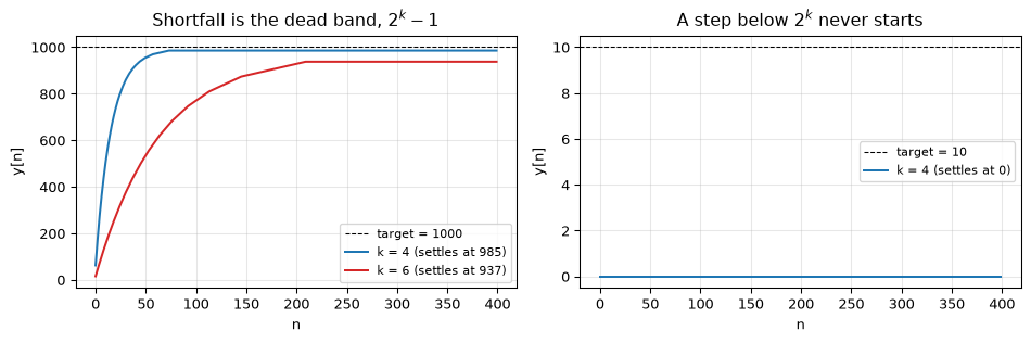
The multiplier-free smoother y += (x - y) >> k is in more embedded codebases than any other filter, and it inherits the flooring directly. The update stalls as soon as the shift of the residual reaches zero, so the filter stops short of its target, permanently, by up to \(2^k - 1\) counts.
Show the code
fig, axes = plt.subplots(1, 2, figsize=(10, 3.4))for ax, (target, ks) inzip(axes, [(1000, (4, 6)), (10, (4,))]): ax.axhline(target, color='k', ls='--', lw=0.8, label=f'target = {target}')for k, c inzip(ks, ('C0', 'C3')): y = ema_shift(np.full(400, target), k)assert y[-1] == ema_shift_final_value(target, k) ax.plot(y, color=c, label=f'k = {k} (settles at {y[-1]})') ax.set_xlabel('n'); ax.set_ylabel('y[n]'); ax.grid(True, alpha=0.3); ax.legend(fontsize=8)axes[0].set_title('Shortfall is the dead band, $2^k - 1$')axes[1].set_title('A step below $2^k$ never starts')fig.tight_layout()plt.show()
Figure 4: Integer EMA y += (x - y) >> k driven by a constant input, rising from zero. The shift-only update stalls once the residual falls below 2^k, leaving a permanent shortfall of up to 2^k - 1 counts on a RISING level (falling, it converges exactly: see the text); a step smaller than the dead band never moves the filter off zero at all.
A step of 10 with \(k=4\) never moves the filter at all: every residual shifts to zero, so the output stays at its initial value forever.
And the dead band is one-sided, which is this section’s own asymmetry turned back on itself. Climbing, the residual is positive and small residuals floor to zero, so the filter stalls short. Falling, the residual is negative, and an arithmetic shift of anything in \([-2^k, -1]\) is \(-1\), never \(0\), so there is no stall at all and the filter converges exactly onto its target. A shift-only EMA tracks a falling level perfectly and a rising one badly. Adding the rounding bias makes the band two-sided and the behaviour symmetric again. This is the same dead-band mechanism as the limit cycles below, reached from the input side rather than the feedback side, and it is why a shift-only EMA should be built with the residual biased ((d + (1 << (k-1))) >> k) or with the state held at a wider fractional width than the output.
A few smaller tricks in the same family
These are not a grab bag. Each is the same move as above: trading an expensive exact operation for a cheap approximate one, and each carries the same kind of debt, paid in bias, in nonlinearity, or in a range you have to check rather than assume.
Choose \(M\) to be a power of two. A moving average over \(M = 2^k\) needs no divider at all, which is why so much embedded smoothing uses window lengths of 16 or 32 rather than 10 or 20. The smoothing embedded page builds exactly this.
Turn constant multiplies into shifts and adds.\(3x = (x \ll 1) + x\); \(0.75x \approx (x \gg 1) + (x \gg 2)\). This is where the rational-approximation question becomes practical: the best small-denominator approximation to a coefficient is a continued-fraction convergent, the same tool used to pick \(L/M\) in rational rate conversion.
Reciprocal multiply, with care. A non-power-of-two divide can become \(x/M \approx (x \cdot R) \gg s\) for a precomputed \(R\). It is what the compiler does to your / 10. But the constant has to be derived, not guessed: the obvious-looking \(R = \lfloor 2^s/M \rfloor + 1\) at \(s = 16\) is exact for \(M = 3\) across \(x \in [0, 20000)\) and wrong on 724 of those same 20 000 inputs for \(M = 5\) (both counts reproduced in the cell below). The correct construction, which compilers use and which is provably exact across the whole range of the input type rather than a range you happened to test, is Granlund and Montgomery’s (Granlund and Montgomery 1994). Reach for that; exhaustive testing is how you confirm a derivation, not a substitute for having one.
Two’s complement has no positive counterpart for its most negative value.-(-32768) is -32768 in int16. In Q15 that is the reason the format holds \(-1.0\) but not \(+1.0\), and the reason a naive abs() in a fixed-point inner loop can hand you back a negative number.
Modelling C in Python needs care in both directions. Python’s // floors, so it matches >>, not /. Python’s int(x/2) truncates, so it matches /, not >>. A Python reference model of embedded C that reaches for // where the C says / will silently disagree on exactly the negative values this section is about.
Show the code
# The reciprocal-multiply counts quoted above, reproduced. Range stated explicitly,# because "a 20 000-sample sweep" is not a specification.XS = np.arange(0, 20000)for M in (3, 5): R = (1<<16) // M +1 bad =int(np.count_nonzero(((XS * R) >>16) != XS // M))print(f"M = {M}: R = {R:>6} mismatches over x in [0, 20000) = {bad}")assert bad == (0if M ==3else724)
M = 3:  R =  21846   mismatches over x in [0, 20000) = 0
M = 5:  R =  13108   mismatches over x in [0, 20000) = 724
Portability footnote
Right-shifting a negative signed integer is implementation-defined in C, and still is. C23 keeps the sentence C99 and C11 used, word for word: “If E1 has a signed type and a negative value, the resulting value is implementation-defined” (ISO/IEC 9899:2024, 6.5.8p5). C++ diverged: since C++20 the standard defines E1 >> E2 for negative E1 as an arithmetic shift, flooring toward minus infinity.
So the flooring this section relies on is guaranteed by the standard only in C++20 and later. In C it is a promise your compiler makes and every mainstream MCU toolchain does make. That is solid ground to build on, but it is the toolchain’s guarantee rather than the language’s, and it is worth one line in your own documentation.
Overflow and scaling
Round-off noise sets the floor; overflow sets the ceiling. In two’s-complement fixed point an intermediate sum that exceeds the range wraps around to a large value of the wrong sign, a far more destructive error than rounding because it is unbounded. A sufficient condition to avoid it at a filter output is
You guarantee that by scaling the input down by a factor \(S\). How hard you scale is a real trade-off, because there are three common bounds of increasing conservativeness (left to right):
The rightmost (the \(\ell_1\) norm) never overflows for any bounded input but is so conservative it throws away dynamic range; the leftmost (\(\ell_2\), energy) is the loosest; the peak-gain bound in the middle is the practical choice for narrowband and sinusoidal signals. And here is the tension that has no free lunch: scaling down to dodge overflow lowers the signal against a fixed noise floor, so it costs SNR. Pick the scaling that just barely avoids overflow for the inputs you actually expect, and no more.
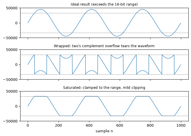
When a value does exceed the range despite scaling, the hardware’s overflow behaviour decides how destructive it is. Plain two’s-complement arithmetic wraps: a value one step past the maximum rolls over to the most negative value, tearing the waveform apart. Saturating arithmetic instead clamps to the nearest representable value, which clips the peaks but keeps the signal recognisable. This is why audio fixed-point code saturates rather than wraps (Yiu 2014, ch. 21):
Show the code
import numpy as npimport matplotlib.pyplot as pltINT16_MIN, INT16_MAX =-32768, 32767n = np.arange(1000)ideal =45000.0* np.sin(2* np.pi *3* n /1000) # exceeds the int16 range# Two's complement wrap: a value past the boundary rolls to the far railwrapped = ((ideal.astype(np.int64) +32768) %65536) -32768# Saturation: clamp to the representable rangesaturated = np.clip(ideal, INT16_MIN, INT16_MAX)# Self-check: wrap injects a near-full-scale jump; saturation never leaves the rangeassert wrapped.max() - wrapped.min() >60000assert saturated.max() <= INT16_MAX and saturated.min() >= INT16_MINfig, axes = plt.subplots(3, 1, figsize=(7, 5), sharex=True)panels = [ (ideal, "Ideal result (exceeds the 16-bit range)"), (wrapped, "Wrapped: two's complement overflow tears the waveform"), (saturated, "Saturated: clamped to the range, mild clipping"),]for ax, (data, title) inzip(axes, panels): ax.plot(n, data, color="C0", lw=1) ax.axhline(INT16_MAX, color="C7", ls="--", lw=0.8) ax.axhline(INT16_MIN, color="C7", ls="--", lw=0.8) ax.set_title(title, fontsize=9) ax.set_ylim(-50000, 50000)axes[-1].set_xlabel("sample n")fig.tight_layout()plt.show()
Figure 5: A signal that exceeds the 16-bit range, handled two ways. Two’s complement wrap (middle) rolls each overflow to the opposite rail, a full-scale discontinuity. Saturation (bottom) clamps to the range, leaving only mild clipping. Dashed lines mark the int16 limits.
No saturating MAC on the Cortex-M4
The Cortex-M4 provides saturating add and subtract (QADD, QSUB) but no saturating multiply-accumulate. A saturating MAC therefore takes two steps, a multiply then a saturating add, costing one extra cycle (Yiu 2014, ch. 21). In tight fixed-point loops the usual practice is the other way around: scale intermediate values down so the accumulator cannot overflow in the first place, and saturate only at the final output.
Limit cycles
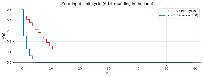
The strangest effect appears only because rounding makes the filter nonlinear. A stable IIR filter should decay to zero once its input stops. With a quantizer in the feedback loop it can instead get stuck, circulating a small nonzero value forever: a granular zero-input limit cycle, granular because the rounding step is what sets its size. It happens when the pole sits close enough to the unit circle that rounding \(a\,y[n-1]\) lands back on \(y[n-1]\), so the decay that should shrink the state never quite does. The dead band is small, on the order of a few quantization steps, but for audio it is an audible idle tone and for a control loop it is a steady-state error that will not go away.
Show the code
near = first_order_zero_input(a=0.9, y0=0.5, n_bits=6, n_samples=60)far = first_order_zero_input(a=0.5, y0=0.5, n_bits=6, n_samples=60)assertabs(near[-1]) > quantization_step(6) and far[-1] ==0.0fig, ax = plt.subplots(figsize=(9, 3.5))ax.step(np.arange(len(near)), near, where='mid', color='C3', label='a = 0.9 (limit cycle)')ax.step(np.arange(len(far)), far, where='mid', color='C0', label='a = 0.5 (decays to 0)')ax.axhline(0, color='k', lw=0.4)ax.set_xlabel('n'); ax.set_ylabel('y[n]'); ax.set_title('Zero-input limit cycle (6-bit rounding in the loop)')ax.legend(fontsize=9); ax.grid(True, alpha=0.3)fig.tight_layout()plt.show()
Figure 6: Zero-input response of the rounding recursion y[n] = Q{a y[n-1]} from the same nonzero start. With the pole near the unit circle (a = 0.9) the state locks into a nonzero limit cycle; with the pole well inside (a = 0.5) it decays cleanly to zero.
Limit cycles are a structure problem too. Some realizations (error-feedback forms, certain wave and lattice structures) are provably free of them; ordinary direct forms are not. As with coefficient sensitivity, the choice of structure decides whether the effect bites. The next section makes that claim precise for the overflow variety, where the argument is clean enough to give a test you can run.
Overflow oscillations, and a test for ruling them out
The limit cycle above is granular: rounding sets its size, and it is a few quantization steps wide. Overflow produces a second kind with the same flavour and a different magnitude. If a sum leaves the representable range the arithmetic must do something with it, and a stable filter can then swing between the rails forever with no input at all (Ebert, Mazo, and Taylor 1969).
The difference equation is the wrong place to study this. It carries one number per step and has no notion of the filter’s internal coordinates, and the coordinates are exactly what overflow acts on, one component at a time. They also differ between realizations of the same transfer function, which the difference equation cannot express at all. So write the filter in state space. With no input, one step is
with \(\mathbf{A}\) the state transition matrix of the realization and \(Q(\cdot)\) the overflow rule. The eigenvalues of \(\mathbf{A}\) are the poles and are the same for every (minimal) realization; \(\mathbf{A}\) itself is not.
An energy that has to shrink
Look for a quadratic form \(V(\mathbf{x}) = \mathbf{x}^{T}\mathbf{D}\,\mathbf{x}\), with \(\mathbf{D}\) positive and diagonal, that decreases at every step. A quantity that strictly decreases cannot return to where it was, so no orbit can persist. It is enough to find one \(\mathbf{D}\) with
because the step splits in two. The linear part shrinks \(V\) by that condition. The overflow part cannot undo it, as long as the arithmetic satisfies \(|Q(v)| \le |v|\) on each component, since \(V\) is then a sum of per-component terms each of which can only shrink.
The diagonality is load-bearing, and it is worth seeing why twice. Concretely: with \(\mathbf{P} = \bigl[\begin{smallmatrix} 0.01 & 0.99 \\ 0.99 & 100\end{smallmatrix}\bigr]\), which is positive definite, and \(\mathbf{v} = (-1.5, 1)\), saturation shrinks both components and \(V\) still rises, from 97.05 to 98.03. The cross term is free to grow while the diagonal terms fall. Structurally: every stable \(\mathbf{A}\) solves \(\mathbf{A}^{T}\mathbf{P}\mathbf{A} - \mathbf{P} = -\mathbf{I}\) for some positive definite \(\mathbf{P}\), so a version of this test quantified over general \(\mathbf{P}\) would certify every stable filter and mean nothing. Diagonality is what makes the condition say more than “the poles are inside the unit circle”.
Which arithmetics qualify, and why wraparound is one of them
The wrap-versus-saturate figure earlier on this page makes wraparound look like the arithmetic that enlarges a value. It does not. Its output is bounded by the range and it is the identity inside the range, so \(|Q(v)| \le |v|\) holds for wraparound exactly as it does for saturation and for magnitude truncation, and the condition above covers all three. This is why the state-space result is usually stated for two’s-complement arithmetic.
What wraparound destroys is sign and continuity: a state a hair over the top of the range reappears at the bottom. Saturation can only ever compress a trajectory towards the rails; wraparound can throw it across the origin and re-launch it. That is a mechanism, not a magnitude, and it is why the two arithmetics can differ on a filter whose \(\mathbf{A}\) carries no certificate.
At second order, the test is the classical result
In direct form the state is a delay line, so \(\mathbf{A}\mathbf{e}_1 = (a_1, 1, 0, \ldots)\) and \(\lVert\mathbf{A}\rVert_2 \ge \sqrt{1 + a_1^{2}} \ge 1\) from second order upward, however deep inside the unit circle the poles sit. Since \(\mathbf{D} = \mathbf{I}\) turns the condition into \(\lVert\mathbf{A}\rVert_2 < 1\), no direct form of order two or more passes at \(\mathbf{D} = \mathbf{I}\).
That is a statement about one \(\mathbf{D}\), not about the test, and the difference matters. Searching over diagonal \(\mathbf{D}\) instead, a second-order direct form does carry a certificate when its coefficients are small enough, and the boundary is not arbitrary:
from finite_wordlength import companion_form, normal_form, lyapunov_margindef has_certificate(A, grid=np.logspace(-4, 4, 801)):"""Is there a diagonal D at all? (Scale-free, so fix the first entry at 1.)"""returnany(lyapunov_margin(A, [1.0, t]) <0for t in grid)rng = np.random.default_rng(0)agree = disagree =0while agree + disagree <400: a1, a2 = rng.uniform(-2.2, 2.2), rng.uniform(-1.05, 1.05)ifabs(a2) >=1orabs(a1) >=1+ a2: # outside the stability trianglecontinueif has_certificate(companion_form([a1, a2])) == (abs(a1) +abs(a2) <1): agree +=1else: disagree +=1print(f"a diagonal D exists <=> |a1| + |a2| < 1 : {agree} agree, {disagree} disagree")assert disagree ==0
a diagonal D exists <=> |a1| + |a2| < 1 : 400 agree, 0 disagree
\(|a_1| + |a_2| < 1\) is the classical condition for a second-order direct form to be free of overflow oscillations. So the state-space test does not sit beside the older second-order theory in some gap of its own: at second order it is that theory, recovered from a matrix inequality that knows nothing about biquads. What the older result adds is the other half of the picture, and it is the half a practitioner uses: with saturating arithmetic a second-order direct form is free of overflow oscillations for any stable coefficients (Ebert, Mazo, and Taylor 1969), including the great majority that fail \(|a_1| + |a_2| < 1\). A resonant biquad with poles near the unit circle fails the certificate comfortably and is still safe, provided the adder saturates.
The normal form passes for every stable pole pair
Write the same pole pair \(r e^{\pm j\theta}\) as a scaled rotation, \(\mathbf{A} = r\,\mathbf{R}(\theta)\). Then \(\mathbf{A}^{T}\mathbf{A} = r^{2}\mathbf{I}\), so \(\lVert\mathbf{A}\rVert_2 = r\) exactly: the pole radius, for any \(\theta\), below one whenever the filter is stable. The certificate is there by construction, with \(\mathbf{D} = \mathbf{I}\).
This is the coupled form that appears at the end of this page as the fix for pole sensitivity near the real axis. The same property rescues both: keeping the state in orthogonal coordinates stops the coefficients from growing, which is what protects the pole positions, and stops \(\lVert\mathbf{A}\rVert_2\) from growing, which is what protects the arithmetic. It is not free. The rotation costs four multiplies per sample in the recursive path where a direct-form biquad costs two, and on a small MCU that is the decision. In exchange both coefficients, \(r\cos\theta\) and \(r\sin\theta\), are bounded by one, where the direct form’s \(a_1\) is not.
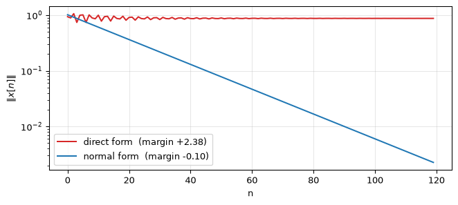
Figure 7: State magnitude with no input and two’s-complement overflow, from the same starting state, for two realizations of one filter (poles at 0.95 exp(+-j pi/4)). Log axis. The direct form settles into a sustained period-2 orbit at about 62% of full scale; the normal form, whose margin is negative, decays as the linear filter says it should.
Above second order, saturation stops being enough
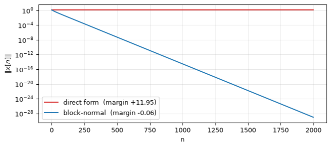
The second-order guarantee does not extend. It is specific to the direct form even at second order: a general stable \(2\times2\) realization can hold a saturating orbit, and at third order the direct form itself can. The coefficients below were found by random search, which is the honest description of how such a filter is located:
Show the code
from finite_wordlength import block_normal_form, saturate, sustains_oscillationa = [2.4364, -2.3099, 0.8597]poles = np.roots(np.concatenate(([1.0], -np.array(a))))A_c, A_b = companion_form(a), block_normal_form(poles)found, orbit = sustains_oscillation(A_c, saturate, seed=11)assert found and orbit_period(orbit) ==6and np.max(np.abs(orbit)) ==1.0start = orbit[0] # one state, both realizationsfig, ax = plt.subplots(figsize=(7, 3.2))for A, name, colour in ((A_c, 'direct form', 'C3'), (A_b, 'block-normal', 'C0')): mag = np.linalg.norm(zero_input_orbit(A, start, saturate, n_samples=2000), axis=1) ax.semilogy(np.maximum(mag, 1e-32), color=colour, label=f'{name} (margin {lyapunov_margin(A):+.2f})')ax.set_xlabel('n'); ax.set_ylabel(r'$\|x[n]\|$'); ax.grid(True, alpha=0.3); ax.legend()fig.tight_layout()plt.show()print(f"max |pole| = {np.abs(poles).max():.4f} (stable: it decays by 29 decades in 2000 samples)")print(f"||A||_2: direct form {np.linalg.norm(A_c, 2):.3f} block-normal {np.linalg.norm(A_b, 2):.4f}")
Figure 8: A stable third-order filter with saturating arithmetic and no input, from one starting state. In direct form the state is trapped in an exactly period-6 orbit at full scale; the block-normal realization of the same three poles decays by 29 orders of magnitude over the same window.
max |pole| = 0.9671  (stable: it decays by 29 decades in 2000 samples)
||A||_2:  direct form 3.599   block-normal 0.9671
The block-normal realization generalizes the rotation: a \(1\times1\) block per real pole, a normal \(2\times2\) block per conjugate pair, giving \(\lVert\mathbf{A}\rVert_2\) equal to the largest pole radius at any order (Barnes and Fam 1977). The state-space condition for realizations of arbitrary order is due to Mills, Mullis and Roberts (Mills, Mullis, and Roberts 1978). Read the logic backwards and the direct form gives up its own verdict: it does oscillate, so no diagonal \(\mathbf{D}\) exists for it, whatever a search might have suggested.
How often does this bite? Over random stable third-order filters, rarely: about 1.5%, and none at all with all poles inside \(|z| = 0.8\), rising to 7.7% for poles between 0.95 and 0.99. But over filters anyone actually designs it is systematic rather than rare, and it appears exactly where this page’s coefficient-sensitivity section already says the direct form is in trouble. A third-order Butterworth lowpass in direct form oscillates for every cutoff at or below \(0.06\,f_s/2\); a Chebyshev-I of the same order, up to \(0.14\). Narrow cutoffs crowd the poles towards \(z = 1\), and that is the region where both effects live.
When to reach for this, and when not to
Rarely, is the honest answer, and the reason is on this page already. Run that same third-order filter the way this page has recommended from its first paragraph, as a cascade of second-order sections with saturating arithmetic, and the problem disappears: from 20000 random starting states the cascade decays to \(4\times10^{-291}\), while the single third-order direct form is trapped at full scale. Factoring into second-order sections and saturating fixes this for free, and it is what you should do.
What the state-space view gives you is not a better default but three things the default cannot supply. It says why the cascade works, in a form that generalizes past the cases anyone has tabulated. It hands you a certificate for a high-order realization you have been given and cannot refactor. And it is the only one of these arguments that survives wraparound, which you meet whenever saturating adds are not available or not affordable.
Three limits, none of them small. This is a zero-input result: what a filter does when a signal drives it into overflow is a separate and harder question, and the original analysis is explicit about leaving it open (Ebert, Mazo, and Taylor 1969). The model applies overflow once per state update, whereas real code either saturates at every adder or accumulates wide and saturates once at the end, and two’s complement in particular is forgiving of intermediate overflow in a way saturation is not, so where you place the nonlinearity changes what is being proved. And the \(\mathbf{D} = \mathbf{I}\) form of the test is not invariant to state scaling: rescale the states of a normal form and its margin can turn positive while a rescaled \(\mathbf{D}\) still certifies it. Scaling, which the earlier section treats as the first line of defence against overflow, is also what decides whether the cheap version of this test answers at all.
Open questions
The overflow test is one-sided, and nothing better is known. A diagonal \(\mathbf{D}\) satisfying the condition above proves no overflow oscillation exists, at any order. Failing it proves nothing: a resonant biquad fails it and is safe anyway under saturation. No tractable necessary-and-sufficient test for an arbitrary realization is available, and the certificate costs roughly double the multiplies in the feedback path, so whether to change structure or to saturate and test remains a judgement call. For granular limit cycles there is no comparable test at all: dead-band bounds exist for first- and second-order sections, and for an arbitrary structure the honest answer is still to simulate and listen.
The noise model is a convenient fiction. Treating quantization error as white, uniform, and uncorrelated with the signal is excellent for busy signals and poor for slowly varying or near-constant ones, where the error becomes signal-dependent and tonal. Dither (deliberately adding a small amount of noise before quantizing) decorrelates the error from the signal, trading a modest increase in the noise floor (about 3 to 5 dB for TPDF) for a clean, distortion-free spectrum. See the dither topic for the full treatment: dither types, the SQNR cost, and when the trade is worth it.
Best structure is filter-specific. Cascade beats direct form for sensitivity, but the ordering and pairing of sections, and which structure minimizes round-off noise, depend on the particular pole-zero constellation. There is no single ordering that is optimal for every filter.
Barnes, C. W., and A. T. Fam. 1977. “Minimum Norm Recursive Digital Filters That Are Free of Overflow Limit Cycles.”IEEE Transactions on Circuits and Systems 24 (10): 569–74.
Gold, Bernard, and Charles M. Rader. 1969. Digital Processing of Signals. McGraw-Hill.
Granlund, Torbjörn, and Peter L. Montgomery. 1994. “Division by Invariant Integers Using Multiplication.” In Proceedings of the ACM SIGPLAN 1994 Conference on Programming Language Design and Implementation (PLDI), 61–72. https://doi.org/10.1145/178243.178249.
Manolakis, Dimitris G., and Vinay K. Ingle. 2011. Applied Digital Signal Processing: Theory and Practice. Cambridge University Press.
Mills, W. L., C. T. Mullis, and R. A. Roberts. 1978. “Digital Filter Realizations Without Overflow Oscillations.”IEEE Transactions on Acoustics, Speech, and Signal Processing 26 (4): 334–38.
Oppenheim, Alan V., and Ronald W. Schafer. 2010. Discrete-Time Signal Processing. 3rd ed. Pearson.
Proakis, John G., and Dimitris G. Manolakis. 2007. Digital Signal Processing: Principles, Algorithms, and Applications. 4th ed. Pearson.
Yiu, Joseph. 2014. The Definitive Guide to ARM Cortex-M3 and Cortex-M4 Processors. 3rd ed. Oxford: Newnes.
Source Code
---title: "Finite Word-Length Effects"subtitle: "What happens to a filter when the bits run out"description-meta: "What happens to a filter when the bits run out: coefficient quantization, rounding noise, overflow, and limit cycles."---On paper a digital filter has infinite precision: its coefficients are real numbers and its arithmetic is exact. On a microcontroller it does not. Coefficients land on a finite grid, every multiply has to be rounded back to the register width, and sums can overflow. These are the **finite word-length effects**, and they are where a design that looks perfect in double precision can degrade, distort, or even go unstable once it meets the metal.This page is the theory companion to the practical fixed-point code in the [biquad embedded page](../../basics/09-biquad/embedded.qmd). It first sets out how fixed-point numbers are represented, then collects the four things that bite, says how big each one is, and shows the structural choices that tame them. The recurring lesson is the same one that motivates [cascaded second-order sections](../../basics/06-filter-design.qmd#second-order-sections): **second-order sections are not a stylistic preference, they are what keeps a fixed-point filter alive.**There are really only a handful of distinct effects:- **Quantization noise** from representing signals and coefficients on a grid.- **Coefficient sensitivity**: the grid moves the poles and zeros, sometimes catastrophically.- **Round-off noise** from rounding every intermediate product.- **Overflow** and the **limit cycles** that nonlinearity can sustain.We take them one at a time. The reference throughout is Manolakis and Ingle [@manolakis2011applied, ch. 15].::: {.callout-note title="Prerequisites"}[The z-domain](../../basics/04-z-domain.qmd) for poles, zeros, and what moving a pole towards the unit circle does to stability; [filter design](../../basics/06-filter-design.qmd) and [filter structures](../../basics/07-filter-structures.qmd) for direct forms and second-order sections, which is the choice this page turns into an arithmetic argument. [Biquad filters](../../basics/09-biquad/index.qmd) and its [embedded page](../../basics/09-biquad/embedded.qmd) are the practical companion: that page writes the fixed-point code, this one says why it is shaped the way it is. The overflow section near the end works in state space; [model-based filtering](../model-based-filtering/index.qmd#the-state-space-model) sets that up if it is unfamiliar.:::::: {.callout-tip title="Code"}The implementation is [`finite_wordlength.py`](finite_wordlength.py). Save [`test_finite_wordlength.py`](test_finite_wordlength.py) beside it and `pytest test_finite_wordlength.py` runs the checks on it.:::```{python}#| echo: falseimport numpy as npimport matplotlib.pyplot as pltfrom scipy import signalfrom finite_wordlength import (quantize, quantization_step, sqnr_db, theoretical_sqnr_db, quantize_coeffs, is_stable, sos_is_stable, first_order_zero_input, shift_scale, c_div_pow2, shift_scale_mean_error, ema_shift, ema_shift_final_value)```<hr>## Quantization noise and the 6 dB per bit ruleRound a signal to a grid of step $\Delta$ and you make an error of at most $\Delta/2$. Model that error as a uniform random variable on $[-\Delta/2, \Delta/2]$ and it has variance$$\sigma_e^2 = \frac{\Delta^2}{12}.$$For a $B$-bit converter spanning the signal range, $\Delta$ halves with every extra bit, so the noise power drops by a factor of four. Against a full-scale sinusoid this gives the headline rule of thumb for the signal-to-quantization-noise ratio,$$\text{SQNR} \approx 6.02\,B + 1.76\ \text{dB},$$about **6 dB, or one bit, of dynamic range per bit of word length**. The demo quantizes a full-scale sine to a range of word lengths and compares the measured SQNR to the formula.```{python}#| label: fig-sqnr#| fig-cap: "Measured signal-to-quantization-noise ratio of a full-scale sinusoid versus word length, against the 6.02B + 1.76 dB rule. The match is within a fraction of a dB."n = np.arange(40000)sine =0.99* np.sin(2* np.pi * n /200) # near-full-scale, no overload from 6 bits upbits = np.arange(6, 17)measured = np.array([sqnr_db(sine, quantize(sine, b)) for b in bits])theory = theoretical_sqnr_db(bits)assert np.max(np.abs(measured - theory)) <1.0# within 1 dB across the sweepfig, ax = plt.subplots(figsize=(8, 4))ax.plot(bits, theory, 'k--', label='6.02B + 1.76 dB')ax.plot(bits, measured, 'o', color='C0', label='measured')ax.set_xlabel('word length B [bits]'); ax.set_ylabel('SQNR [dB]')ax.set_title('Quantization noise: 6 dB per bit')ax.legend(fontsize=9); ax.grid(True, alpha=0.3)fig.tight_layout()plt.show()```This is the budget you start from: a 12-bit ADC gives you about 74 dB to work with, a 16-bit one about 98 dB. Everything below eats into it.<hr>## Fixed-point representation: Q-formatsWhen the target has no floating-point unit (a Cortex-M0+, an AVR) or when power and throughput demand the integer path, signals and coefficients are stored as scaled integers in **Q-format**. A Q$m$.$n$ number is a two's-complement integer read as having $n$ fractional bits; the two common audio choices both represent a value in $[-1, 1)$:| Format | Bits | Range | Resolution | Use case ||--------|------|-------|------------|----------|| Q15 | 16 | $[-1,\ 1 - 2^{-15})$ | $3.05 \times 10^{-5}$ | Low-power, small filters || Q31 | 32 | $[-1,\ 1 - 2^{-31})$ | $4.66 \times 10^{-10}$ | High-quality audio |A coefficient stored in Q15 is an integer in $[-32768, 32767]$ standing for $\text{integer}/32768$, and all arithmetic stays in the integer domain. The programmer's job is to track where the binary point lands after each operation: a Q15 times Q15 product is Q30 (it has 30 fractional bits in 32), so it must be shifted back before it is stored or summed. Coefficients that exceed $\pm 1$ (a high-gain peaking EQ, for instance) do not fit Q15 at all and must be pre-scaled, with a compensating gain applied elsewhere. This bookkeeping is the price of dropping the FPU, and it is why the [biquad embedded page](../../basics/09-biquad/embedded.qmd) leans on CMSIS-DSP's ready-made Q15 and Q31 filters rather than rolling the arithmetic by hand.<hr>## Coefficient quantization: the poles moveQuantizing the *signal* adds noise. Quantizing the *coefficients* does something more dangerous: it changes the filter. Each coefficient is forced onto the grid,$$\hat{a}_k = a_k + \Delta a_k, \qquad \hat{b}_k = b_k + \Delta b_k,$$and those perturbations move the poles and zeros. A sensitivity analysis [@manolakis2011applied, eq. 15.70] shows that the shift of pole $p_i$ depends on $1/\prod_{j\neq i}(p_i - p_j)$: when poles are **tightly clustered**, as they are in a narrowband or high-order filter, that denominator is tiny and the poles are exquisitely sensitive. Implement such a filter as one high-order direct-form transfer function and quantization can fling a pole clean outside the unit circle.The cure is structural. Split the filter into [second-order sections](../../basics/06-filter-design.qmd#second-order-sections): each section holds one conjugate pole pair, its two coefficients stay in $[-2, 2]$, and the pole of one section no longer depends on the coefficients of the others. The demo takes a 5th-order elliptic bandpass and quantizes its coefficients two ways.```{python}#| label: fig-coeff-quant#| fig-cap: "A 5th-order elliptic bandpass under 10-bit coefficient quantization. As one direct-form (b, a) transfer function (left) three of its conjugate pole pairs are pushed outside the unit circle and the filter is unstable. As cascaded second-order sections (right) the same word length leaves every pole in place."order, wn = signal.ellipord([0.3, 0.4], [0.2, 0.5], 0.1, 60)b, a = signal.ellip(order, 0.1, 60, wn, btype='band')sos = signal.ellip(order, 0.1, 60, wn, btype='band', output='sos')n_bits =10c_max =2** np.ceil(np.log2(np.max(np.abs(a)) +1.0)) # direct form needs many integer bitsa_q = quantize_coeffs(np.asarray(a), n_bits, c_max=c_max)b_q = quantize_coeffs(np.asarray(b), n_bits, c_max=c_max)sos_q = np.array([quantize_coeffs(s, n_bits, c_max=2.0) for s in sos])# The whole point, checked at render time:assert is_stable(a) andnot is_stable(a_q) and sos_is_stable(sos_q)print(f"direct form needs c_max = {c_max:.0f} (|a| up to {np.max(np.abs(a)):.1f}); "f"quantized direct form stable? {is_stable(a_q)}; quantized SOS stable? {sos_is_stable(sos_q)}")def poles_ba(a):return np.roots(a)def poles_sos(sos):return np.concatenate([np.roots(s[3:6]) for s in np.atleast_2d(sos)])fig, axes = plt.subplots(1, 2, figsize=(10, 5))theta = np.linspace(0, 2* np.pi, 400)for ax, p_inf, p_q, title in [ (axes[0], poles_ba(a), poles_ba(a_q), f'Direct form, {n_bits}-bit'), (axes[1], poles_sos(sos), poles_sos(sos_q), f'Cascade (SOS), {n_bits}-bit')]: ax.plot(np.cos(theta), np.sin(theta), 'k-', linewidth=0.7) ax.plot(p_inf.real, p_inf.imag, 'o', mfc='none', mec='C7', label='infinite precision') ax.plot(p_q.real, p_q.imag, 'x', color='C3', label='quantized') ax.set_title(title); ax.set_xlabel('Re'); ax.set_ylabel('Im') ax.set_aspect('equal'); ax.set_xlim(-1.6, 1.6); ax.set_ylim(-1.4, 1.4) ax.axhline(0, color='k', lw=0.3); ax.axvline(0, color='k', lw=0.3) ax.grid(True, alpha=0.3); ax.legend(fontsize=8, loc='upper left')fig.tight_layout()plt.show()```The direct form fails not only because its poles are clustered but because its coefficients have a huge dynamic range (the denominator coefficients of a 10th-degree polynomial run into the tens), so at a fixed word length the grid spacing on them is coarse. The cascade form keeps every coefficient small and every pole independent. This is the numerical argument behind the [biquad](../../basics/09-biquad/index.qmd) chapter, made quantitative.<hr>## Round-off noise and the accumulatorEven with the poles safely placed, every multiply inside the filter produces a full-width product that has to be rounded back to the register, and each rounding injects a fresh $\Delta^2/12$ of noise. For a length-$(M{+}1)$ FIR filter that rounds after every tap, the noise powers add and the output noise variance is$$\sigma_g^2 = (M+1)\,\frac{\Delta^2}{12},$$so a longer filter is a noisier one. The fix is the **double-width accumulator**: keep the running sum at full precision and round only once, at the very end. Then a single quantizer contributes and the output noise collapses to$$\sigma_g^2 = \frac{\Delta^2}{12},$$independent of filter length. This is exactly why DSP cores carry a **wide accumulator**: a $B$-bit by $B$-bit product is about $2B$ bits, so the running sum is kept at double width plus a few guard bits, and often much wider (CMSIS-DSP's Q15 biquads accumulate in 64 bits). The same point is made in passing on the [biquad embedded page](../../basics/09-biquad/embedded.qmd) and quantified here.```{python}#| label: fig-roundoff#| fig-cap: "Output round-off noise of a length-33 FIR filter. Rounding once in a wide accumulator matches the Delta^2/12 floor almost exactly; rounding after every tap is roughly an order of magnitude noisier (the (M+1) model is an upper estimate, since the small per-tap products do not fully exercise the quantizer)."rng = np.random.default_rng(0)M1 =33# number of tapsh = signal.firwin(M1, 0.25)B =8delta = quantization_step(B)x = (2* rng.random(20000) -1) *0.9# full-ish scale random inputexact = np.convolve(x, h) # full, infinite-precision reference# round after every tap: M+1 quantizers, summed in one aligned frameper_tap = np.zeros(len(exact))for k inrange(M1): contrib = np.zeros(len(exact)) contrib[k:k +len(x)] = h[k] * x per_tap += quantize(contrib, B)single = quantize(exact, B) # wide accumulator: sum exactly, round onceinterior =slice(M1, len(x)) # region where all taps are activevar_per_tap = np.var((per_tap - exact)[interior])var_single = np.var((single - exact)[interior])pred_single = delta**2/12assert0.5< var_single / pred_single <2.0# single quantizer hits the floorassert var_per_tap >8* var_single # per-tap is far noisierprint(f"single-quantizer noise var {var_single:.2e} (Delta^2/12 = {pred_single:.2e})")print(f"per-tap noise var {var_per_tap:.2e}")print(f"wide accumulator is {var_per_tap / var_single:.0f}x quieter for {M1} taps")fig, ax = plt.subplots(figsize=(6, 3.5))ax.bar(['per-tap\n(M+1 quantizers)', 'wide accumulator\n(1 quantizer)'], [var_per_tap, var_single], color=['C3', 'C0'])ax.axhline(pred_single, color='k', linestyle='--', linewidth=0.8, label=r'$\Delta^2/12$ floor')ax.set_yscale('log'); ax.set_ylabel('output noise variance')ax.set_title('Round-off noise: where you round matters')ax.legend(fontsize=8); ax.grid(True, alpha=0.3, axis='y')fig.tight_layout()plt.show()```<hr>## Dividing without a divider: scaling by shiftsEverything above assumes you can round. On the metal you often cannot afford to, because **division is expensive**. The smallest targets on the capability ladder have no hardware divider at all (the ATmega328P, and ARMv6-M cores such as the Cortex-M0+); ARMv7-M cores like the Cortex-M4 do provide `SDIV`/`UDIV`, but at 2 to 12 cycles (data-dependent, early-terminating) against 1 for an add or a shift, it is still among the slowest integer instructions they have, per the Cortex-M4 Technical Reference Manual. So the standing advice for integer DSP is to **design every scaling to be a power of two**, then implement it with a right shift.That advice is sound, and it comes with a trap that is easy to state and easy to miss:$$(-n) \gg 1 \;\neq\; -(n \gg 1).$$A right shift **floors** (rounds toward $-\infty$); C's `/` **truncates** (rounds toward zero). On non-negative values the two agree, which is why the bug survives testing on a unipolar signal and appears the moment real bipolar audio arrives.```{python}x = np.array([-5, -3, -1, 0, 1, 3, 5])print("x ", x)print("x >> 1 ", shift_scale(x, 1)) # floorsprint("x / 2 (C)", c_div_pow2(x, 1)) # truncates toward zero# The identity above, concretely: (-1) >> 1 is -1, while -(1 >> 1) is 0.assert shift_scale(np.array([-1]), 1)[0] ==-1assert-shift_scale(np.array([1]), 1)[0] ==0```### The part that matters: a shift is a biased quantizerThe [round-off model above](#round-off-noise-and-the-accumulator) treats quantization error as uniform on $[-\Delta/2, \Delta/2]$, and therefore **zero-mean**. That is true of rounding. It is not true of a shift. Discarding the low $k$ bits leaves an error that is uniform on $\{0, -1/2^k, \ldots, -(2^k-1)/2^k\}$, whose mean is$$\mu_\gg = -\frac{2^k - 1}{2^{k+1}} \;\xrightarrow[k \to \infty]{}\; -\frac{1}{2}\ \text{LSB},$$while its variance still tends to $\Delta^2/12$. Both figures assume the discarded low bits are busy enough to be uniform, which is the same standing caveat the [open questions](#open-questions) below attach to the rounding model, inherited here rather than escaped. So a shift costs you **the same noise power as rounding, plus a DC offset of up to half an LSB**. That is the seam between algorithm design and implementation: the noise budget you computed on paper survives, and a bias you never budgeted for appears underneath it.The usual fix is to add half an output LSB before shifting, `(x + (1 << (k-1))) >> k`, which makes ties round up. It does not remove the bias, it replaces it:$$\mu_{\gg,\text{rounded}} = +\frac{1}{2^{k+1}}.$$At $k=1$ that is $+0.25$ LSB, exactly as bad as the $-0.25$ it replaced. It only pays off as $k$ grows, which is the case that matters: by $k=8$ the bias is $+1/512$ LSB instead of $-1/2$. Genuinely unbiased rounding needs round-half-to-even, which costs more logic than most inner loops will give up.```{python}rng = np.random.default_rng(0)xr = rng.integers(-(1<<20), 1<<20, size=1<<18)print(f"{'k':>3}{'shift mean':>11}{'closed form':>12}{'biased mean':>12} "f"{'closed form':>12}{'variance':>9}")for k in (1, 4, 8, 15): exact = xr / (1<< k) e_shift = shift_scale(xr, k) - exact e_round = shift_scale(xr, k, rounded=True) - exactprint(f"{k:>3}{e_shift.mean():>11.5f}{shift_scale_mean_error(k):>12.5f} "f"{e_round.mean():>12.5f}{shift_scale_mean_error(k, rounded=True):>12.5f} "f"{e_shift.var():>9.5f}")# The claims of this section, checked at render time.assertabs(e_shift.mean() - shift_scale_mean_error(k)) <0.01assertabs(e_round.mean() - shift_scale_mean_error(k, rounded=True)) <0.01print(f"\nDelta^2/12 = {1/12:.5f}")```The measured means track the closed forms across the sweep. At $k=15$ the *biased* column is the exception: its true value, $1/65536$, is below the Monte Carlo error of a $2^{18}$-sample estimate (about $6 \times 10^{-4}$), so what that row reports is the noise floor of the measurement, not a disagreement with the formula.Note the contrast with C's `/`, which is **unbiased** on symmetric data because its rounding direction follows the sign. It buys that at the price of being nonlinear: it has a dead zone straddling zero, where both $+1$ and $-1$ scale to $0$. Neither operator is simply correct. The shift is linear with an offset; the divide is unbiased with a kink. Pick the error your signal chain can absorb.### The same trap, one level up: the shift-only EMAThe multiplier-free smoother `y += (x - y) >> k` is in more embedded codebases than any other filter, and it inherits the flooring directly. The update stalls as soon as the shift of the residual reaches zero, so the filter **stops short of its target**, permanently, by up to $2^k - 1$ counts.```{python}#| label: fig-shift-ema#| fig-cap: "Integer EMA y += (x - y) >> k driven by a constant input, rising from zero. The shift-only update stalls once the residual falls below 2^k, leaving a permanent shortfall of up to 2^k - 1 counts on a RISING level (falling, it converges exactly: see the text); a step smaller than the dead band never moves the filter off zero at all."fig, axes = plt.subplots(1, 2, figsize=(10, 3.4))for ax, (target, ks) inzip(axes, [(1000, (4, 6)), (10, (4,))]): ax.axhline(target, color='k', ls='--', lw=0.8, label=f'target = {target}')for k, c inzip(ks, ('C0', 'C3')): y = ema_shift(np.full(400, target), k)assert y[-1] == ema_shift_final_value(target, k) ax.plot(y, color=c, label=f'k = {k} (settles at {y[-1]})') ax.set_xlabel('n'); ax.set_ylabel('y[n]'); ax.grid(True, alpha=0.3); ax.legend(fontsize=8)axes[0].set_title('Shortfall is the dead band, $2^k - 1$')axes[1].set_title('A step below $2^k$ never starts')fig.tight_layout()plt.show()```A step of 10 with $k=4$ never moves the filter at all: every residual shifts to zero, so the output stays at its initial value forever.**And the dead band is one-sided**, which is this section's own asymmetry turned back on itself. Climbing, the residual is positive and small residuals floor to zero, so the filter stalls short. *Falling*, the residual is negative, and an arithmetic shift of anything in $[-2^k, -1]$ is $-1$, never $0$, so there is no stall at all and the filter converges exactly onto its target. A shift-only EMA tracks a falling level perfectly and a rising one badly. Adding the rounding bias makes the band two-sided and the behaviour symmetric again. This is the same dead-band mechanism as the [limit cycles](#limit-cycles) below, reached from the input side rather than the feedback side, and it is why a shift-only EMA should be built with the residual biased (`(d + (1 << (k-1))) >> k`) or with the state held at a wider fractional width than the output.### A few smaller tricks in the same familyThese are not a grab bag. Each is the same move as above: trading an expensive exact operation for a cheap approximate one, and each carries the same kind of debt, paid in bias, in nonlinearity, or in a range you have to check rather than assume.- **Choose $M$ to be a power of two.** A moving average over $M = 2^k$ needs no divider at all, which is why so much embedded smoothing uses window lengths of 16 or 32 rather than 10 or 20. The [smoothing embedded page](../../basics/08-smoothing/embedded.qmd) builds exactly this.- **Turn constant multiplies into shifts and adds.** $3x = (x \ll 1) + x$; $0.75x \approx (x \gg 1) + (x \gg 2)$. This is where the rational-approximation question becomes practical: the best small-denominator approximation to a coefficient is a continued-fraction convergent, the same tool used to pick $L/M$ in [rational rate conversion](../../basics/10-multirate/index.qmd#rational-rate-conversion).- **Reciprocal multiply, with care.** A non-power-of-two divide can become $x/M \approx (x \cdot R) \gg s$ for a precomputed $R$. It is what the compiler does to your `/ 10`. But the constant has to be *derived*, not guessed: the obvious-looking $R = \lfloor 2^s/M \rfloor + 1$ at $s = 16$ is exact for $M = 3$ across $x \in [0, 20000)$ and wrong on 724 of those same 20 000 inputs for $M = 5$ (both counts reproduced in the cell below). The correct construction, which compilers use and which is provably exact across the *whole* range of the input type rather than a range you happened to test, is Granlund and Montgomery's [@granlund1994division]. Reach for that; exhaustive testing is how you confirm a derivation, not a substitute for having one.- **Two's complement has no positive counterpart for its most negative value.** `-(-32768)` is `-32768` in `int16`. In Q15 that is the reason the format holds $-1.0$ but not $+1.0$, and the reason a naive `abs()` in a fixed-point inner loop can hand you back a negative number.- **Modelling C in Python needs care in both directions.** Python's `//` floors, so it matches `>>`, not `/`. Python's `int(x/2)` truncates, so it matches `/`, not `>>`. A Python reference model of embedded C that reaches for `//` where the C says `/` will silently disagree on exactly the negative values this section is about.```{python}# The reciprocal-multiply counts quoted above, reproduced. Range stated explicitly,# because "a 20 000-sample sweep" is not a specification.XS = np.arange(0, 20000)for M in (3, 5): R = (1<<16) // M +1 bad =int(np.count_nonzero(((XS * R) >>16) != XS // M))print(f"M = {M}: R = {R:>6} mismatches over x in [0, 20000) = {bad}")assert bad == (0if M ==3else724)```::: {.callout-note}## Portability footnoteRight-shifting a *negative* signed integer is **implementation-defined in C, and still is**. C23 keeps the sentence C99 and C11 used, word for word: *"If E1 has a signed type and a negative value, the resulting value is implementation-defined"* (ISO/IEC 9899:2024, 6.5.8p5). C++ diverged: since C++20 the standard defines `E1 >> E2` for negative `E1` as an arithmetic shift, flooring toward minus infinity.So the flooring this section relies on is guaranteed by the standard only in C++20 and later. In C it is a promise your compiler makes and every mainstream MCU toolchain does make. That is solid ground to build on, but it is the toolchain's guarantee rather than the language's, and it is worth one line in your own documentation.:::<hr>## Overflow and scalingRound-off noise sets the floor; **overflow** sets the ceiling. In two's-complement fixed point an intermediate sum that exceeds the range wraps around to a large value of the wrong sign, a far more destructive error than rounding because it is unbounded. A sufficient condition to avoid it at a filter output is$$|y[n]| = \left|\sum_k h[k]\,x[n-k]\right| \le \sum_k |h[k]|\,|x[n-k]| < 1.$$You guarantee that by scaling the input down by a factor $S$. How hard you scale is a real trade-off, because there are three common bounds of increasing conservativeness (left to right):$$\Bigl(\textstyle\sum_k |h[k]|^2\Bigr)^{1/2} \;\le\; \max_\omega |H(e^{j\omega})| \;\le\; \sum_k |h[k]|.$$The rightmost (the $\ell_1$ norm) never overflows for *any* bounded input but is so conservative it throws away dynamic range; the leftmost ($\ell_2$, energy) is the loosest; the peak-gain bound in the middle is the practical choice for narrowband and sinusoidal signals. And here is the tension that has no free lunch: **scaling down to dodge overflow lowers the signal against a fixed noise floor, so it costs SNR.** Pick the scaling that just barely avoids overflow for the inputs you actually expect, and no more.When a value does exceed the range despite scaling, the hardware's overflow behaviour decides how destructive it is. Plain two's-complement arithmetic **wraps**: a value one step past the maximum rolls over to the most negative value, tearing the waveform apart. **Saturating** arithmetic instead clamps to the nearest representable value, which clips the peaks but keeps the signal recognisable. This is why audio fixed-point code saturates rather than wraps [@yiu2014, ch. 21]:```{python}#| label: fig-wrap-vs-saturate#| fig-cap: "A signal that exceeds the 16-bit range, handled two ways. Two's complement wrap (middle) rolls each overflow to the opposite rail, a full-scale discontinuity. Saturation (bottom) clamps to the range, leaving only mild clipping. Dashed lines mark the int16 limits."import numpy as npimport matplotlib.pyplot as pltINT16_MIN, INT16_MAX =-32768, 32767n = np.arange(1000)ideal =45000.0* np.sin(2* np.pi *3* n /1000) # exceeds the int16 range# Two's complement wrap: a value past the boundary rolls to the far railwrapped = ((ideal.astype(np.int64) +32768) %65536) -32768# Saturation: clamp to the representable rangesaturated = np.clip(ideal, INT16_MIN, INT16_MAX)# Self-check: wrap injects a near-full-scale jump; saturation never leaves the rangeassert wrapped.max() - wrapped.min() >60000assert saturated.max() <= INT16_MAX and saturated.min() >= INT16_MINfig, axes = plt.subplots(3, 1, figsize=(7, 5), sharex=True)panels = [ (ideal, "Ideal result (exceeds the 16-bit range)"), (wrapped, "Wrapped: two's complement overflow tears the waveform"), (saturated, "Saturated: clamped to the range, mild clipping"),]for ax, (data, title) inzip(axes, panels): ax.plot(n, data, color="C0", lw=1) ax.axhline(INT16_MAX, color="C7", ls="--", lw=0.8) ax.axhline(INT16_MIN, color="C7", ls="--", lw=0.8) ax.set_title(title, fontsize=9) ax.set_ylim(-50000, 50000)axes[-1].set_xlabel("sample n")fig.tight_layout()plt.show()```::: {.callout-note title="No saturating MAC on the Cortex-M4"}The Cortex-M4 provides saturating add and subtract (`QADD`, `QSUB`) but no saturating multiply-accumulate. A saturating MAC therefore takes two steps, a multiply then a saturating add, costing one extra cycle [@yiu2014, ch. 21]. In tight fixed-point loops the usual practice is the other way around: scale intermediate values down so the accumulator cannot overflow in the first place, and saturate only at the final output.:::<hr>## Limit cyclesThe strangest effect appears only because rounding makes the filter **nonlinear**. A stable IIR filter should decay to zero once its input stops. With a quantizer in the feedback loop it can instead get stuck, circulating a small nonzero value forever: a **granular zero-input limit cycle**, granular because the rounding step is what sets its size. It happens when the pole sits close enough to the unit circle that rounding $a\,y[n-1]$ lands back on $y[n-1]$, so the decay that should shrink the state never quite does. The dead band is small, on the order of a few quantization steps, but for audio it is an audible idle tone and for a control loop it is a steady-state error that will not go away.```{python}#| label: fig-limit-cycle#| fig-cap: "Zero-input response of the rounding recursion y[n] = Q{a y[n-1]} from the same nonzero start. With the pole near the unit circle (a = 0.9) the state locks into a nonzero limit cycle; with the pole well inside (a = 0.5) it decays cleanly to zero."near = first_order_zero_input(a=0.9, y0=0.5, n_bits=6, n_samples=60)far = first_order_zero_input(a=0.5, y0=0.5, n_bits=6, n_samples=60)assertabs(near[-1]) > quantization_step(6) and far[-1] ==0.0fig, ax = plt.subplots(figsize=(9, 3.5))ax.step(np.arange(len(near)), near, where='mid', color='C3', label='a = 0.9 (limit cycle)')ax.step(np.arange(len(far)), far, where='mid', color='C0', label='a = 0.5 (decays to 0)')ax.axhline(0, color='k', lw=0.4)ax.set_xlabel('n'); ax.set_ylabel('y[n]'); ax.set_title('Zero-input limit cycle (6-bit rounding in the loop)')ax.legend(fontsize=9); ax.grid(True, alpha=0.3)fig.tight_layout()plt.show()```Limit cycles are a structure problem too. Some realizations (error-feedback forms, certain wave and lattice structures) are provably free of them; ordinary direct forms are not. As with coefficient sensitivity, the choice of structure decides whether the effect bites. The next section makes that claim precise for the *overflow* variety, where the argument is clean enough to give a test you can run.<hr>## Overflow oscillations, and a test for ruling them outThe limit cycle above is **granular**: rounding sets its size, and it is a few quantization steps wide. Overflow produces a second kind with the same flavour and a different magnitude. If a sum leaves the representable range the arithmetic must do *something* with it, and a stable filter can then swing between the rails forever with no input at all [@ebert1969overflow].The difference equation is the wrong place to study this. It carries one number per step and has no notion of the filter's internal coordinates, and the coordinates are exactly what overflow acts on, one component at a time. They also differ between realizations of the same transfer function, which the difference equation cannot express at all. So write the filter in **state space**. With no input, one step is$$\mathbf{x}[n+1] = Q\!\left(\mathbf{A}\,\mathbf{x}[n]\right)$$with $\mathbf{A}$ the state transition matrix of the realization and $Q(\cdot)$ the overflow rule. The eigenvalues of $\mathbf{A}$ are the poles and are the same for every (minimal) realization; $\mathbf{A}$ itself is not.### An energy that has to shrinkLook for a quadratic form $V(\mathbf{x}) = \mathbf{x}^{T}\mathbf{D}\,\mathbf{x}$, with $\mathbf{D}$ positive and **diagonal**, that decreases at every step. A quantity that strictly decreases cannot return to where it was, so no orbit can persist. It is enough to find one $\mathbf{D}$ with$$\mathbf{A}^{T}\mathbf{D}\,\mathbf{A} - \mathbf{D} \prec 0$$because the step splits in two. The linear part shrinks $V$ by that condition. The overflow part cannot undo it, as long as the arithmetic satisfies $|Q(v)| \le |v|$ on each component, since $V$ is then a sum of per-component terms each of which can only shrink.**The diagonality is load-bearing, and it is worth seeing why twice.** Concretely: with $\mathbf{P} = \bigl[\begin{smallmatrix} 0.01 & 0.99 \\ 0.99 & 100\end{smallmatrix}\bigr]$, which is positive definite, and $\mathbf{v} = (-1.5, 1)$, saturation shrinks *both* components and $V$ still rises, from 97.05 to 98.03. The cross term is free to grow while the diagonal terms fall. Structurally: every stable $\mathbf{A}$ solves $\mathbf{A}^{T}\mathbf{P}\mathbf{A} - \mathbf{P} = -\mathbf{I}$ for some positive definite $\mathbf{P}$, so a version of this test quantified over general $\mathbf{P}$ would certify every stable filter and mean nothing. Diagonality is what makes the condition say more than "the poles are inside the unit circle".::: {.callout-note title="Which arithmetics qualify, and why wraparound is one of them"}The wrap-versus-saturate figure earlier on this page makes wraparound look like the arithmetic that *enlarges* a value. It does not. Its output is bounded by the range and it is the identity inside the range, so $|Q(v)| \le |v|$ holds for wraparound exactly as it does for saturation and for magnitude truncation, and the condition above covers all three. This is why the state-space result is usually stated for two's-complement arithmetic.What wraparound destroys is sign and continuity: a state a hair over the top of the range reappears at the bottom. Saturation can only ever compress a trajectory towards the rails; wraparound can throw it across the origin and re-launch it. That is a mechanism, not a magnitude, and it is why the two arithmetics can differ on a filter whose $\mathbf{A}$ carries no certificate.:::### At second order, the test is the classical resultIn direct form the state is a delay line, so $\mathbf{A}\mathbf{e}_1 = (a_1, 1, 0, \ldots)$ and $\lVert\mathbf{A}\rVert_2 \ge \sqrt{1 + a_1^{2}} \ge 1$ from second order upward, however deep inside the unit circle the poles sit. Since $\mathbf{D} = \mathbf{I}$ turns the condition into $\lVert\mathbf{A}\rVert_2 < 1$, **no direct form of order two or more passes at $\mathbf{D} = \mathbf{I}$.**That is a statement about one $\mathbf{D}$, not about the test, and the difference matters. Searching over diagonal $\mathbf{D}$ instead, a second-order direct form does carry a certificate when its coefficients are small enough, and the boundary is not arbitrary:```{python}#| code-fold: falsefrom finite_wordlength import companion_form, normal_form, lyapunov_margindef has_certificate(A, grid=np.logspace(-4, 4, 801)):"""Is there a diagonal D at all? (Scale-free, so fix the first entry at 1.)"""returnany(lyapunov_margin(A, [1.0, t]) <0for t in grid)rng = np.random.default_rng(0)agree = disagree =0while agree + disagree <400: a1, a2 = rng.uniform(-2.2, 2.2), rng.uniform(-1.05, 1.05)ifabs(a2) >=1orabs(a1) >=1+ a2: # outside the stability trianglecontinueif has_certificate(companion_form([a1, a2])) == (abs(a1) +abs(a2) <1): agree +=1else: disagree +=1print(f"a diagonal D exists <=> |a1| + |a2| < 1 : {agree} agree, {disagree} disagree")assert disagree ==0```$|a_1| + |a_2| < 1$ is the classical condition for a second-order direct form to be free of overflow oscillations. So the state-space test does not sit beside the older second-order theory in some gap of its own: at second order it **is** that theory, recovered from a matrix inequality that knows nothing about biquads. What the older result adds is the other half of the picture, and it is the half a practitioner uses: with **saturating** arithmetic a second-order direct form is free of overflow oscillations for *any* stable coefficients [@ebert1969overflow], including the great majority that fail $|a_1| + |a_2| < 1$. A resonant biquad with poles near the unit circle fails the certificate comfortably and is still safe, provided the adder saturates.### The normal form passes for every stable pole pairWrite the same pole pair $r e^{\pm j\theta}$ as a scaled rotation, $\mathbf{A} = r\,\mathbf{R}(\theta)$. Then $\mathbf{A}^{T}\mathbf{A} = r^{2}\mathbf{I}$, so $\lVert\mathbf{A}\rVert_2 = r$ exactly: the pole radius, for any $\theta$, below one whenever the filter is stable. The certificate is there by construction, with $\mathbf{D} = \mathbf{I}$.This is the coupled form that appears at the end of this page as the fix for pole sensitivity near the real axis. The same property rescues both: keeping the state in orthogonal coordinates stops the coefficients from growing, which is what protects the pole positions, and stops $\lVert\mathbf{A}\rVert_2$ from growing, which is what protects the arithmetic. It is not free. The rotation costs four multiplies per sample in the recursive path where a direct-form biquad costs two, and on a small MCU that is the decision. In exchange both coefficients, $r\cos\theta$ and $r\sin\theta$, are bounded by one, where the direct form's $a_1$ is not.```{python}#| label: fig-overflow-wrap#| fig-cap: "State magnitude with no input and two's-complement overflow, from the same starting state, for two realizations of one filter (poles at 0.95 exp(+-j pi/4)). Log axis. The direct form settles into a sustained period-2 orbit at about 62% of full scale; the normal form, whose margin is negative, decays as the linear filter says it should."from finite_wordlength import wrap, zero_input_orbit, orbit_periodr, theta =0.95, np.pi /4A_direct = companion_form([2* r * np.cos(theta), -r**2])A_normal = normal_form(r, theta)x0 = np.array([0.9, -0.6])fig, ax = plt.subplots(figsize=(7, 3.2))for A, name, colour in ((A_direct, 'direct form', 'C3'), (A_normal, 'normal form', 'C0')): mag = np.linalg.norm(zero_input_orbit(A, x0, wrap, n_samples=120), axis=1) ax.semilogy(np.maximum(mag, 1e-18), color=colour, label=f'{name} (margin {lyapunov_margin(A):+.2f})')ax.set_xlabel('n'); ax.set_ylabel(r'$\|x[n]\|$'); ax.grid(True, alpha=0.3); ax.legend()fig.tight_layout()plt.show()steady = zero_input_orbit(A_direct, x0, wrap, n_samples=60, n_settle=20000)assert orbit_period(steady) ==2assert0.61< np.max(np.abs(steady)) <0.62assert np.max(np.abs(zero_input_orbit(A_normal, x0, wrap, n_samples=20, n_settle=20000))) <1e-12```### Above second order, saturation stops being enoughThe second-order guarantee does not extend. It is specific to the direct form even at second order: a general stable $2\times2$ realization can hold a saturating orbit, and at third order the direct form itself can. The coefficients below were found by random search, which is the honest description of how such a filter is located:```{python}#| label: fig-overflow-sat#| fig-cap: "A stable third-order filter with saturating arithmetic and no input, from one starting state. In direct form the state is trapped in an exactly period-6 orbit at full scale; the block-normal realization of the same three poles decays by 29 orders of magnitude over the same window."from finite_wordlength import block_normal_form, saturate, sustains_oscillationa = [2.4364, -2.3099, 0.8597]poles = np.roots(np.concatenate(([1.0], -np.array(a))))A_c, A_b = companion_form(a), block_normal_form(poles)found, orbit = sustains_oscillation(A_c, saturate, seed=11)assert found and orbit_period(orbit) ==6and np.max(np.abs(orbit)) ==1.0start = orbit[0] # one state, both realizationsfig, ax = plt.subplots(figsize=(7, 3.2))for A, name, colour in ((A_c, 'direct form', 'C3'), (A_b, 'block-normal', 'C0')): mag = np.linalg.norm(zero_input_orbit(A, start, saturate, n_samples=2000), axis=1) ax.semilogy(np.maximum(mag, 1e-32), color=colour, label=f'{name} (margin {lyapunov_margin(A):+.2f})')ax.set_xlabel('n'); ax.set_ylabel(r'$\|x[n]\|$'); ax.grid(True, alpha=0.3); ax.legend()fig.tight_layout()plt.show()print(f"max |pole| = {np.abs(poles).max():.4f} (stable: it decays by 29 decades in 2000 samples)")print(f"||A||_2: direct form {np.linalg.norm(A_c, 2):.3f} block-normal {np.linalg.norm(A_b, 2):.4f}")```The block-normal realization generalizes the rotation: a $1\times1$ block per real pole, a normal $2\times2$ block per conjugate pair, giving $\lVert\mathbf{A}\rVert_2$ equal to the largest pole radius at any order [@barnes1977minimum]. The state-space condition for realizations of arbitrary order is due to Mills, Mullis and Roberts [@mills1978digital]. Read the logic backwards and the direct form gives up its own verdict: it *does* oscillate, so no diagonal $\mathbf{D}$ exists for it, whatever a search might have suggested.How often does this bite? Over random stable third-order filters, rarely: about **1.5%**, and **none at all** with all poles inside $|z| = 0.8$, rising to 7.7% for poles between 0.95 and 0.99. But over filters anyone actually designs it is systematic rather than rare, and it appears exactly where this page's coefficient-sensitivity section already says the direct form is in trouble. A third-order Butterworth lowpass in direct form oscillates for every cutoff at or below $0.06\,f_s/2$; a Chebyshev-I of the same order, up to $0.14$. Narrow cutoffs crowd the poles towards $z = 1$, and that is the region where both effects live.### When to reach for this, and when not toRarely, is the honest answer, and the reason is on this page already. Run that same third-order filter the way this page has recommended from its first paragraph, as a cascade of second-order sections with saturating arithmetic, and the problem disappears: from 20000 random starting states the cascade decays to $4\times10^{-291}$, while the single third-order direct form is trapped at full scale. **Factoring into second-order sections and saturating fixes this for free, and it is what you should do.**What the state-space view gives you is not a better default but three things the default cannot supply. It says *why* the cascade works, in a form that generalizes past the cases anyone has tabulated. It hands you a certificate for a high-order realization you have been given and cannot refactor. And it is the only one of these arguments that survives wraparound, which you meet whenever saturating adds are not available or not affordable.Three limits, none of them small. This is a **zero-input** result: what a filter does when a signal drives it into overflow is a separate and harder question, and the original analysis is explicit about leaving it open [@ebert1969overflow]. The model applies overflow once per state update, whereas real code either saturates at every adder or accumulates wide and saturates once at the end, and two's complement in particular is forgiving of *intermediate* overflow in a way saturation is not, so where you place the nonlinearity changes what is being proved. And the $\mathbf{D} = \mathbf{I}$ form of the test is not invariant to state scaling: rescale the states of a normal form and its margin can turn positive while a rescaled $\mathbf{D}$ still certifies it. Scaling, which the earlier section treats as the first line of defence against overflow, is also what decides whether the cheap version of this test answers at all.<hr>## Open questions- **The overflow test is one-sided, and nothing better is known.** A diagonal $\mathbf{D}$ satisfying the condition above proves no overflow oscillation exists, at any order. Failing it proves nothing: a resonant biquad fails it and is safe anyway under saturation. No tractable necessary-and-sufficient test for an arbitrary realization is available, and the certificate costs roughly double the multiplies in the feedback path, so whether to change structure or to saturate and test remains a judgement call. For *granular* limit cycles there is no comparable test at all: dead-band bounds exist for first- and second-order sections, and for an arbitrary structure the honest answer is still to simulate and listen.- **The noise model is a convenient fiction.** Treating quantization error as white, uniform, and uncorrelated with the signal is excellent for busy signals and poor for slowly varying or near-constant ones, where the error becomes signal-dependent and tonal. Dither (deliberately adding a small amount of noise before quantizing) decorrelates the error from the signal, trading a modest increase in the noise floor (about 3 to 5 dB for TPDF) for a clean, distortion-free spectrum. See the [dither topic](../dither/index.qmd) for the full treatment: dither types, the SQNR cost, and when the trade is worth it.- **Best structure is filter-specific.** Cascade beats direct form for sensitivity, but the *ordering* and *pairing* of sections, and which structure minimizes round-off noise, depend on the particular pole-zero constellation. There is no single ordering that is optimal for every filter.<hr>## ReferencesThe treatment follows Manolakis and Ingle [@manolakis2011applied, ch. 15]; see also Oppenheim and Schafer [@oppenheim2010discrete] and Proakis and Manolakis [@proakis2007digital]. The coupled-form structure that reduces pole sensitivity near the real axis is due to Gold and Rader [@goldrader1969].::: {#refs}:::