Decimation, interpolation, and sample rate conversion
Nature’s multirate system
The human retina is a biological multirate system: the fovea (central 2 degrees) samples at extremely high spatial resolution, while the periphery progressively decimates, trading resolution for wider coverage (Curcio et al. 1990). This is the same bandwidth-efficiency trade-off that drives digital multirate processing: sample densely where detail matters, decimate where it doesn’t.
Sampling a signal at 1 MHz when you only need 10 kHz of bandwidth wastes storage, bus bandwidth, and processing cycles. Conversely, converting audio between 44.1 kHz and 48 kHz (two sample rates that exist because the CD and professional audio industries could not agree on a standard) requires changing the rate by a non-integer factor. Multirate signal processing provides the tools to move between sample rates efficiently and correctly. For the embedded side (CIC filters, CMSIS-DSP polyphase decimation, and two-stage pipelines on STM32F4 and ESP32-S3), see Multirate on Hardware.
The applications are everywhere. Sigma-delta ADCs oversample at many times the Nyquist rate, then decimate digitally to achieve high resolution with simple analog front-ends. Software-defined radios digitise wide bands at high rates, then decimate to isolate narrow channels. Audio equipment routinely converts between 44.1, 48, 88.2, 96, and 192 kHz. In all these cases, the core operations are the same: decimation, interpolation, and the filters that make them work.
Prerequisites
This topic assumes familiarity with the frequency domain (particularly spectral effects of sampling) and filter design (anti-aliasing and FIR design).
Code
The implementation is multirate.py. Save test_multirate.py beside it and pytest test_multirate.py runs the checks on it.
Decimation (downsampling)
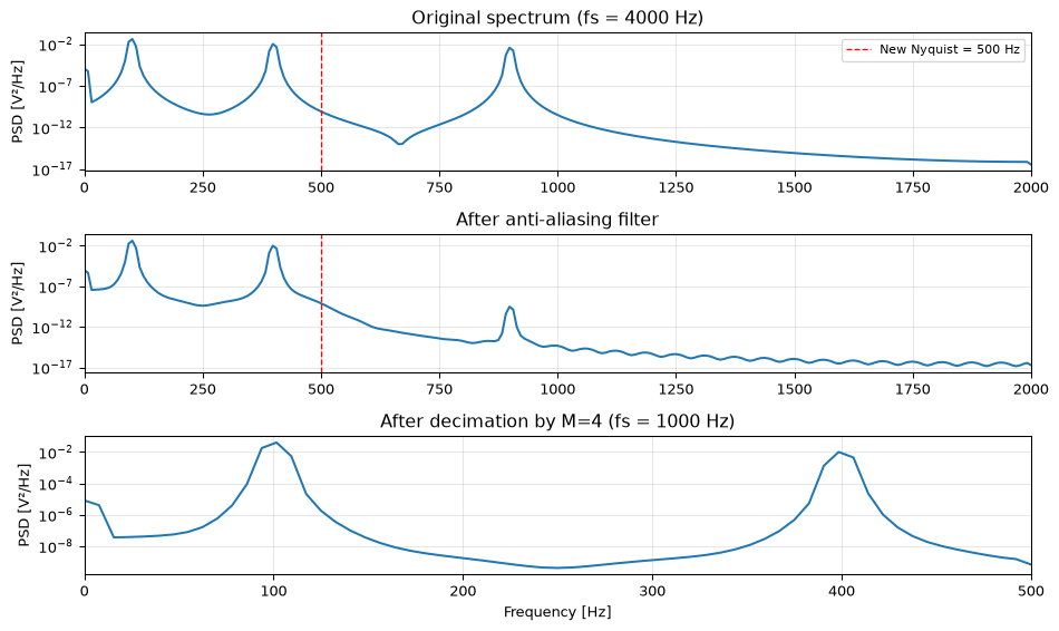
Decimation reduces the sample rate by an integer factor \(M\): keep every \(M\)-th sample, discard the rest. But you cannot simply throw away samples. That would alias any spectral content above the new Nyquist frequency \(f_s / (2M)\) back into the baseband.
The correct procedure is:
Anti-aliasing filter: a lowpass filter with cutoff \(f_s / (2M)\)
Downsample by \(M\): keep every \(M\)-th sample
The output sample rate is \(f_s / M\), and the anti-aliasing filter ensures that no aliased components fold into the output band.
Mathematically, if \(x[n]\) is filtered to produce \(x_f[n]\), the decimated output is:
\[y[m] = x_f[mM]\]
In the frequency domain, downsampling by \(M\) causes spectral folding. The DTFT of the decimated signal is:
The \(M\) shifted copies of the spectrum overlap; without the anti-aliasing filter, they alias destructively.
Show the code
import numpy as npimport matplotlib.pyplot as pltfrom scipy import signal as sig# Create a test signal: sum of sinusoids at 100, 400, and 900 Hzfs =4000N =2000t = np.arange(N) / fsx = np.sin(2* np.pi *100* t) +0.5* np.sin(2* np.pi *400* t) +0.3* np.sin(2* np.pi *900* t)M =4fs_new = fs // M# Anti-aliasing filter: lowpass at fs/(2M) = 500 Hzb_aa = sig.firwin(65, 1.0/ M)x_filtered = sig.lfilter(b_aa, 1.0, x)# Decimatex_dec = x_filtered[::M]fig, axes = plt.subplots(3, 1, figsize=(10, 6))# Original spectrumf_orig, Pxx_orig = sig.welch(x, fs, nperseg=512)axes[0].semilogy(f_orig, Pxx_orig)axes[0].set_title(f'Original spectrum (fs = {fs} Hz)')axes[0].set_ylabel('PSD [V²/Hz]')axes[0].axvline(fs_new /2, color='r', linestyle='--', linewidth=1, label=f'New Nyquist = {fs_new//2} Hz')axes[0].legend(fontsize=8)# After anti-aliasing filterf_filt, Pxx_filt = sig.welch(x_filtered, fs, nperseg=512)axes[1].semilogy(f_filt, Pxx_filt)axes[1].set_title('After anti-aliasing filter')axes[1].set_ylabel('PSD [V²/Hz]')axes[1].axvline(fs_new /2, color='r', linestyle='--', linewidth=1)# After decimationf_dec, Pxx_dec = sig.welch(x_dec, fs_new, nperseg=128)axes[2].semilogy(f_dec, Pxx_dec)axes[2].set_title(f'After decimation by M={M} (fs = {fs_new} Hz)')axes[2].set_ylabel('PSD [V²/Hz]')axes[2].set_xlabel('Frequency [Hz]')for ax in axes: ax.set_xlim(0, fs /2) ax.grid(True, alpha=0.3)axes[2].set_xlim(0, fs_new /2)fig.tight_layout()plt.show()
Figure 1: Decimation by M=4. Top: original signal spectrum. Middle: after anti-aliasing filter. Bottom: after downsampling, the spectrum is stretched by M, filling the new Nyquist band.
SciPy provides scipy.signal.decimate, which handles the anti-aliasing filter and downsampling in one call. By default it uses a Chebyshev Type I IIR filter, though FIR is often preferable for multirate work (the ftype='fir' option).
Interpolation (upsampling)
Interpolation increases the sample rate by an integer factor \(L\). The procedure mirrors decimation:
Upsample by \(L\): insert \(L-1\) zeros between each sample
Anti-imaging filter: a lowpass filter with cutoff \(f_s / 2\) (the original Nyquist, equivalently \(f_{s,\text{out}}/(2L)\)) and gain \(L\)
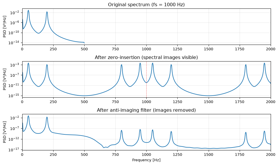
The zero-insertion step creates \(L-1\) spectral images (copies of the baseband spectrum centred at multiples of the original sample rate). The anti-imaging filter removes these images, leaving only the baseband.
The upsampled signal before filtering is:
\[x_u[n] = \begin{cases} x[n/L] & \text{if } n \text{ is a multiple of } L \\ 0 & \text{otherwise} \end{cases}\]
Its spectrum contains \(L\) copies of the original:
\[X_u(e^{j\omega}) = X(e^{j\omega L})\]
The anti-imaging filter passes only the copy centred at DC and applies a gain of \(L\) to restore the correct amplitude.
Show the code
# Original signal at low ratefs_low =1000N_low =500t_low = np.arange(N_low) / fs_lowx_low = np.sin(2* np.pi *50* t_low) +0.5* np.sin(2* np.pi *200* t_low)L =4fs_high = fs_low * L# Zero insertionx_up = np.zeros(N_low * L)x_up[::L] = x_low# Anti-imaging filter (gain = L to compensate for zero insertion)b_ai = sig.firwin(65, 1.0/ L) * Lx_interp = sig.lfilter(b_ai, 1.0, x_up)fig, axes = plt.subplots(3, 1, figsize=(10, 6))# Original spectrumf1, P1 = sig.welch(x_low, fs_low, nperseg=256)axes[0].semilogy(f1, P1)axes[0].set_title(f'Original spectrum (fs = {fs_low} Hz)')axes[0].set_ylabel('PSD [V²/Hz]')# After zero insertion, show full Nyquist band of the upsampled ratef2, P2 = sig.welch(x_up, fs_high, nperseg=1024)axes[1].semilogy(f2, P2)axes[1].set_title(f'After zero-insertion (spectral images visible)')axes[1].set_ylabel('PSD [V²/Hz]')for k inrange(1, L): axes[1].axvline(k * fs_low, color='r', linestyle='--', linewidth=0.8, alpha=0.5)# After anti-imaging filterf3, P3 = sig.welch(x_interp, fs_high, nperseg=1024)axes[2].semilogy(f3, P3)axes[2].set_title('After anti-imaging filter (images removed)')axes[2].set_ylabel('PSD [V²/Hz]')axes[2].set_xlabel('Frequency [Hz]')for ax in axes: ax.set_xlim(0, fs_high /2) ax.grid(True, alpha=0.3)fig.tight_layout()plt.show()
Figure 2: Interpolation by L=4. Top: original spectrum. Middle: after zero-insertion, spectral images appear at multiples of the original fs. Bottom: after anti-imaging filter removes the images.
Rational rate conversion
What if you need to convert from 44.1 kHz to 48 kHz? The ratio is \(48000/44100 = 160/147\): neither a pure integer upsample nor downsample. The solution is to interpolate by \(L\) then decimate by \(M\), where \(L/M\) equals the desired rate ratio:
The key insight is that the interpolation and decimation filters can be combined into a single filter. Both require a lowpass: the interpolation filter has cutoff \(\pi/L\) and the decimation filter has cutoff \(\pi/M\). The combined filter uses the more restrictive of the two:
In practice, scipy.signal.resample_poly(x, L, M) does this efficiently. It designs the combined anti-aliasing/anti-imaging FIR filter and uses polyphase decomposition internally so that computation is proportional to the output length, not the high intermediate rate \(L \cdot f_s\).
Show the code
# Simulate a short audio segment at 44.1 kHzfs_in =44100duration =0.05# 50 mst_in = np.arange(int(fs_in * duration)) / fs_inx_in = np.sin(2* np.pi *440* t_in) +0.3* np.sin(2* np.pi *1000* t_in)# Rational SRCL, M =160, 147fs_out = fs_in * L // M # 48000x_out = sig.resample_poly(x_in, L, M)t_out = np.arange(len(x_out)) / fs_outfig, axes = plt.subplots(2, 1, figsize=(10, 4))axes[0].plot(t_in *1000, x_in, '.-', markersize=2, linewidth=0.5)axes[0].set_title(f'Input: {fs_in} Hz ({len(x_in)} samples)')axes[0].set_ylabel('Amplitude')axes[1].plot(t_out *1000, x_out, '.-', markersize=2, linewidth=0.5, color='C1')axes[1].set_title(f'Output: {fs_out} Hz ({len(x_out)} samples)')axes[1].set_ylabel('Amplitude')axes[1].set_xlabel('Time [ms]')for ax in axes: ax.set_xlim(0, 10) # Show first 10 ms ax.grid(True, alpha=0.3)fig.tight_layout()plt.show()
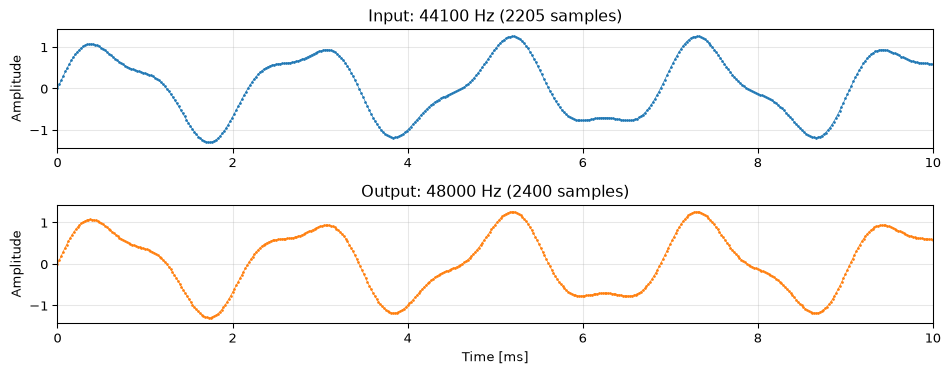
Figure 3: Rational sample rate conversion: 44.1 kHz to 48 kHz using L=160, M=147. The signal content is preserved while the sample rate changes.
The 44.1 vs 48 kHz problem
The 44.1/48 kHz conversion is the classic multirate problem in audio. 44,100 Hz was chosen for the CD standard (derived from video line rates), while 48,000 Hz became the professional audio and broadcast standard. Every time audio moves between consumer and professional domains (DAWs, streaming services, broadcast chains) this conversion happens. The ratio 160/147 is not close to any small integer, so the polyphase filter is long. Getting this conversion transparent (no audible artifacts) is a solved problem, but it took decades of engineering.
A related experiment: play a 44.1 kHz recording at 48 kHz without resampling. Every sample is interpreted as occurring \(48000/44100 \approx 1.088\) times too fast, so pitch shifts up by about 1.5 semitones and duration shrinks by 8.1% (\(1 - 44100/48000\)). The Beethoven demo in DSP2 course material uses this to dramatic effect: a symphony in the wrong key.
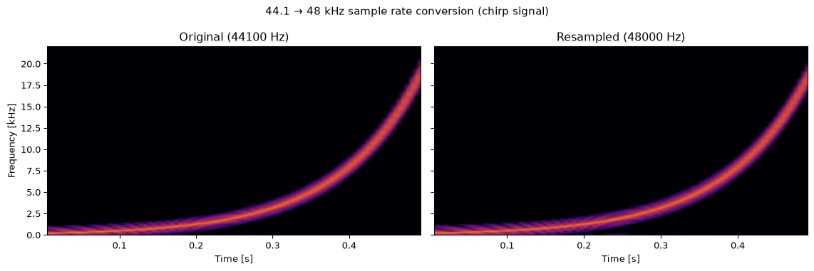
The following demo generates a chirp signal, resamples it from 44.1 to 48 kHz using resample_poly, and compares the spectrograms to verify that spectral content is preserved without aliasing artifacts.
Show the code
import numpy as npimport matplotlib.pyplot as pltfrom scipy import signal as sig# Generate a chirp at 44.1 kHz: sweep from 200 Hz to 20 kHz over 0.5 sfs_441 =44100duration =0.5t_441 = np.arange(int(fs_441 * duration)) / fs_441chirp = sig.chirp(t_441, f0=200, f1=20000, t1=duration, method='logarithmic')# Resample to 48 kHzL, M =160, 147fs_48 =48000chirp_48 = sig.resample_poly(chirp, L, M)t_48 = np.arange(len(chirp_48)) / fs_48fig, axes = plt.subplots(1, 2, figsize=(12, 4), sharey=True)nperseg =512for ax, x, fs_val, title in [ (axes[0], chirp, fs_441, f'Original ({fs_441} Hz)'), (axes[1], chirp_48, fs_48, f'Resampled ({fs_48} Hz)')]: f, t_spec, Sxx = sig.spectrogram(x, fs_val, nperseg=nperseg, noverlap=nperseg//2) ax.pcolormesh(t_spec, f /1000, 10* np.log10(Sxx +1e-12), shading='gouraud', cmap='inferno', vmin=-80, vmax=0) ax.set_xlabel('Time [s]') ax.set_title(title) ax.set_ylim(0, 22)axes[0].set_ylabel('Frequency [kHz]')fig.suptitle('44.1 → 48 kHz sample rate conversion (chirp signal)', fontsize=11)fig.tight_layout()plt.show()
Figure 4: Resampling a chirp from 44.1 kHz to 48 kHz. The spectrogram shows the frequency sweep is preserved cleanly, no aliasing, no spectral artifacts.
Choosing \(L\) and \(M\) when the ratio is not exact
The \(160/147\) above is exact: both rates are integers you control, so dividing out \(\gcd(48000, 44100) = 300\) gives the ratio with nothing left over. That is the easy case, and it is not the general one. Two free-running clocks drift apart by tens of parts per million, and plenty of real conversions have no small exact ratio at all. Then \(L/M\) is something you choose, and the choice is a trade.
The trade is this: you need a fraction close enough to the true ratio, but with a denominator small enough to build, because \(M\) and \(L\) set the filter’s size. So the question is not “what is the ratio?” but “what is the closest fraction I can afford?”
That question has an exact answer, and the tool is the continued fraction expansion. Writing a number as a nested fraction and stopping early gives a sequence of approximations called convergents, and each one is optimal for its size: no fraction with a smaller denominator comes closer. Python has this built in as Fraction.limit_denominator, which takes the largest denominator you are willing to pay for and returns the best fraction within that budget. The bound you hand it is a hardware budget, because \(L\) is the number of polyphase branches you are about to build.
Show the code
from fractions import Fractionimport math# Two nominally-matched clocks, 50 ppm apart. The true ratio is no longer 160/147.true_ratio =48000/ (44100* (1+50e-6))print(f"target ratio = {true_ratio:.12f}\n")print(f"{'max denom':>10}{'L / M':>12}{'branches L':>11}{'error (ppm)':>13}{'cents':>8}")for q in (10, 50, 147, 1000, 10000): f = Fraction(true_ratio).limit_denominator(q) err = (float(f) - true_ratio) / true_ratio cents =1200* math.log2(1+ err)print(f"{q:>10}{str(f):>12}{f.numerator:>11}{err*1e6:>13.3f}{cents:>8.3f}")# The textbook answer is itself just a convergent, and it is not the cheapest one.assert Fraction(true_ratio).limit_denominator(1000).numerator ==665assert Fraction(48000, 44100) == Fraction(160, 147)
target ratio = 1.088380955102

 max denom        L / M  branches L   error (ppm)    cents
        10        11/10          11     10675.531   18.384
        50        37/34          37      -133.833   -0.232
       147      160/147         160        50.000    0.087
      1000      665/611         665        -1.148   -0.002
     10000    2857/2625        2857        -0.002   -0.000
Two things fall out of that table. The first is that \(160/147\) is itself only a convergent of the drifted ratio, not a privileged answer: it lands 50 ppm off, which is precisely the clock error, because it is the nominal ratio. Buying a further 43x reduction in rate error, about one and a half more decimal digits of agreement, costs you \(L = 665\) branches instead of 160.
The second runs the other way, and it is the useful one. Going down to \(L = 37\) (\(37/34\)) leaves a rate error of about 134 ppm, roughly a quarter of a cent of pitch shift, while cutting the polyphase bank by more than a factor of four. For a one-off file conversion that is an excellent trade: a quarter of a cent sits well under ordinary pitch discrimination, which runs to several cents even for a practised ear. The exact threshold depends on the listener, the register and the test, so treat the margin as comfortable rather than as a specific number.
A rate error does not stay small in a live stream
That trade holds for a finite signal. On a continuous link between two independently clocked devices, a constant rate error accumulates: at 134 ppm the streams slip by one sample roughly every 7500 samples, about six times a second at 44.1 kHz. No fixed \(L/M\) can fix that, because the ratio you are trying to match is itself drifting. Live links need asynchronous sample rate conversion, where the ratio is measured continuously and the resampler is steered by a feedback loop. Continued fractions choose a good fixed ratio; they do not remove the need for that loop.
Polyphase decomposition
The naive approach to interpolation by \(L\) is expensive: insert zeros, then filter at the high rate \(L \cdot f_s\). But \(L-1\) out of every \(L\) input samples to the filter are zero, so most of the multiply-accumulate operations produce nothing. Polyphase decomposition eliminates this waste (Crochiere and Rabiner 1983).
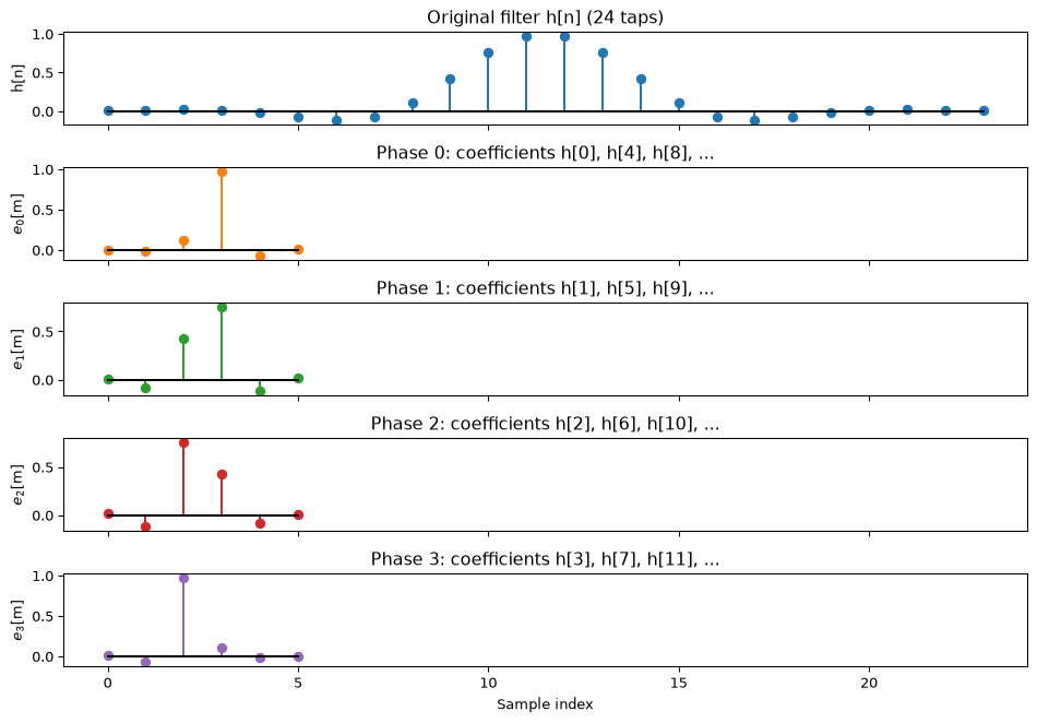
The idea is to split the filter \(H(z)\) of length \(N\) into \(L\) subfilters (phases), each of length \(N/L\):
\[H(z) = \sum_{k=0}^{L-1} z^{-k} E_k(z^L)\]
where the \(k\)-th polyphase component contains every \(L\)-th coefficient:
Each subfilter \(E_k\) operates at the low sample rate. The outputs are interleaved to form the high-rate signal. The computational cost drops by a factor of \(L\) compared to the direct approach.
For decimation, the same principle applies in reverse: the input is split into \(M\) polyphase components (a commutator distributing successive input samples to \(M\) branches), each branch is filtered at the low rate, and the outputs are summed.
Figure 5: Polyphase decomposition of a 24-tap FIR filter into L=4 subfilters. Each subfilter operates at the low sample rate, reducing computation by a factor of L.
Tip
SciPy’s resample_poly uses polyphase decomposition internally. You get the efficiency gains without implementing the decomposition yourself. For custom implementations (e.g., on embedded hardware), the polyphase structure maps naturally to a round-robin of short FIR filters.
Multi-stage decimation
Decimating by a large factor \(M\) in a single stage requires a very sharp anti-aliasing filter: the transition band must be narrow relative to the output bandwidth. For \(M = 100\) with \(f_s = 100\) kHz, the anti-aliasing filter needs a cutoff at 500 Hz with a transition band of a few hundred Hz at most. This requires thousands of taps.
Multi-stage decimation breaks the operation into cascaded stages with smaller decimation factors. For \(M = 100\):
Single stage: \(\div 100\) (very sharp filter, very expensive)
Two stages: \(\div 10 \to \div 10\) (two moderate filters, much cheaper)
Why is this more efficient? Each subsequent stage operates at a lower sample rate, so its filter runs fewer multiply-accumulates per second. And the transition band requirements are relaxed: each stage only needs to prevent aliasing down to its own output Nyquist frequency, not the final one.
The total number of multiplications per output sample for a cascade is typically much less than for a single stage. The optimal number of stages and the factor split depend on the specific \(M\) and the required stopband attenuation, and finding the optimal decomposition is itself an interesting design problem.
A worked complexity comparison
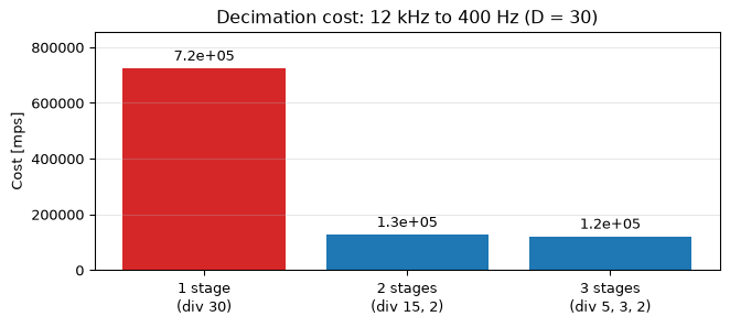
Put numbers on it. Decimate a signal from \(f_s = 12\) kHz down to 400 Hz, so \(D = 30\), with an anti-aliasing filter specified by passband edge \(f_{pb} = 180\) Hz, stopband edge \(f_{sb} = 200\) Hz, passband ripple \(\delta_{pb} = 0.002\), and stopband ripple \(\delta_{sb} = 0.001\). Kaiser’s estimate for the FIR length is
and the cost of a polyphase FIR decimator is \(C = N\,f_s/D\) multiplications per second (mps), since the filter runs at the output rate.
Single stage (\(\div 30\)). The transition band is razor thin, \(\Delta f = 20/12000 \approx 0.0017\), so \(N \approx 1809\) taps and \(C \approx 7.2 \times 10^5\) mps.
Two stages (\(\div 15\) then \(\div 2\)). The first filter \(F\) runs at 12 kHz but only has to keep aliasing out of the final 200 Hz passband. Its own output rate is \(f_s/D_1 = 800\) Hz, so its spectrum folds around 800 Hz; the highest input frequency that could land inside the final 200 Hz passband after that fold sits at \(f_s/D_1 - f_s/(2D) = 800 - 200 = 600\) Hz. So \(F\)’s stopband need only start at 600 Hz: a luxuriously wide transition. The second filter \(G\) does the sharp \(180 \to 200\) Hz cut, but at 800 Hz instead of 12 kHz. One more bookkeeping point: passband ripples roughly add through a cascade, so to hold the overall \(\delta_{pb} = 0.002\) we hand each of two stages \(0.001\) (and each of three stages about \(0.00067\)). With that, \(N_F \approx 93\) and \(N_G \approx 130\), for a combined \(C \approx 1.3 \times 10^5\) mps. About six times cheaper.
Three stages (\(\div 5\), \(\div 3\), \(\div 2\)). The first two stages relax even further (\(N_R \approx 21\), \(N_S \approx 20\)), but the final sharp filter \(N_T \approx 135\) now dominates the total, \(C \approx 1.2 \times 10^5\) mps. Barely better than two stages: once the cheap early decimation is done, the unavoidable sharp final cut sets the floor, and adding stages chases diminishing returns.
Figure 6: Total decimation cost for one, two, and three stages of a 12 kHz -> 400 Hz (D=30) decimator. The big win is single -> two stages; the third stage barely helps because the sharp final filter dominates.
CIC filters
The Cascaded Integrator-Comb (CIC) filter is a special case of multi-stage decimation that uses no multiplications at all. A CIC of order \(K\) decimating by \(M\) is:
In the efficient decimator, the \(K\) integrators \(1/(1 - z^{-1})\) run at the high input rate, and the \(K\) combs run at the low output rate: the Noble identity lets each comb move across the downsampler, where the high-rate \((1 - z^{-M})\) becomes a cheap single-delay \((1 - z^{-1})\). Both stages use only additions and subtractions.
Crucially, each integrator is a running sum kept as a recursion, acc += x, not an \(M\)-tap sum recomputed every output. So the cost is a fixed handful of adds per sample no matter how large \(M\) is, and there are no multipliers anywhere (Lyons 2005). That combination is why the CIC is the filter of choice at the brutal sample rates right after a fast ADC.
Where the CIC lives: the digital down-converter
The classic home is the radio receiver. An RF or IF signal is sampled fast (tens to hundreds of MHz), mixed down to baseband by a numerically-controlled oscillator, and then decimated to the actual channel bandwidth. That decimation chain is the digital down-converter (DDC):
The CIC sits first, right after the mixer, precisely because it runs at that punishing input rate where a multiply-based FIR would be unaffordable. It knocks the rate down cheaply; the sharp, multiply-heavy filtering then happens downstream at the low rate where you can afford it. (The mixer and NCO are a communications-systems topic in their own right; here we care only about the rate-conversion filter.) The transmit side is the mirror image, a digital up-converter that interpolates with a CIC before the DAC. CIC filters are equally at home decimating the raw bitstream from a sigma-delta ADC (Hogenauer 1981); the modulator that produces that bitstream, built from the same integrator and differentiator blocks, is dissected in the ADC noise topic.
The price: sinc droop and finite alias rejection
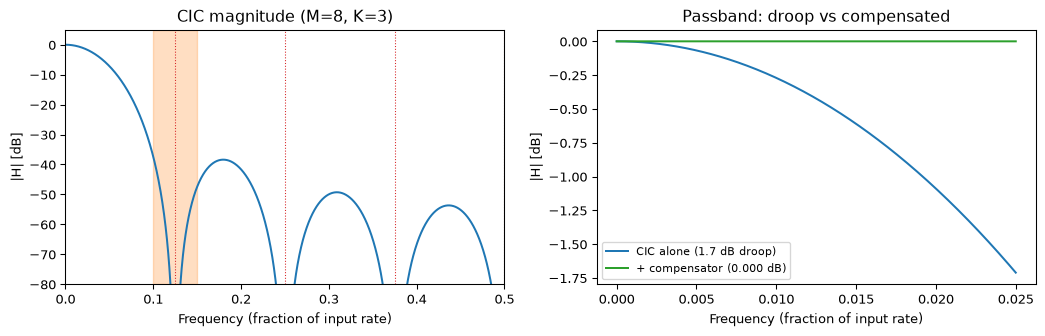
Nothing is free. The CIC’s frequency response is a sinc-like shape: nulls at every multiple of the output rate \(f_{s,\text{in}}/M\) (which is exactly where the aliasing bands fold from, so the nulls do useful work), but also a drooping passband and only finite stopband rejection. Both get worse as you ask more of the filter.
Show the code
from multirate import cic_response, cic_compensatorM, K =8, 3fc =0.4# passband edge as a fraction of output Nyquistf_out =1.0/ M # output rate, as a fraction of the input ratef_pb = fc * f_out /2# passband edge, in input-rate fraction# Full-band CIC magnitude (high-rate frequency, normalised to unity DC gain)f = np.linspace(0, 0.5, 2000)Om =2* np.pi * fmag = np.ones_like(Om); nz = Om >0mag[nz] = np.abs(np.sin(M * Om[nz] /2) / (M * np.sin(Om[nz] /2))) ** K# Passband droop, worst-case alias rejection, and compensationw = np.linspace(0, fc * np.pi, 512) # output-rate frequency over the passbandcic_pb = cic_response(w, M, K)droop_db =20* np.log10(cic_pb.max() / cic_pb.min())alias_edge = f_out - f_pb # near edge of the first folding bandrej_db =-20* np.log10(mag[np.argmin(np.abs(f - alias_edge))])h = cic_compensator(M, K, num_taps=9, fc=fc)comp = np.abs(h @ np.exp(-1j* np.outer(np.arange(len(h)), w)))combined = cic_pb * compripple_db =20* np.log10(combined.max() / combined.min())assert1.6< droop_db <1.8# ~1.71 dB of droopassert36< rej_db <39# ~37 dB worst-case alias rejectionassert ripple_db <0.001# compensator flattens it to < a thousandth of a dBprint(f"passband droop {droop_db:.2f} dB -> {ripple_db:.3f} dB after a 9-tap compensator")print(f"worst-case alias rejection {rej_db:.1f} dB at the first folding band")fig, (axL, axR) = plt.subplots(1, 2, figsize=(11, 3.6))axL.plot(f, 20* np.log10(mag +1e-9), 'C0')for k inrange(1, M //2+1): axL.axvline(k / M, color='C3', ls=':', lw=0.8)axL.axvspan(alias_edge, f_out + f_pb, color='C1', alpha=0.25)axL.set_xlim(0, 0.5); axL.set_ylim(-80, 5)axL.set_xlabel('Frequency (fraction of input rate)'); axL.set_ylabel('|H| [dB]')axL.set_title(f'CIC magnitude (M={M}, K={K})')f_axis = w / np.pi * f_out /2# map output-rate frequency back to input-rate fractionaxR.plot(f_axis, 20* np.log10(cic_pb), 'C0', label=f'CIC alone ({droop_db:.1f} dB droop)')axR.plot(f_axis, 20* np.log10(combined), 'C2', label=f'+ compensator ({ripple_db:.3f} dB)')axR.set_xlabel('Frequency (fraction of input rate)'); axR.set_ylabel('|H| [dB]')axR.set_title('Passband: droop vs compensated'); axR.legend(fontsize=8)fig.tight_layout(); plt.show()
passband droop 1.71 dB -> 0.000 dB after a 9-tap compensator
worst-case alias rejection 37.5 dB at the first folding band
Figure 7: Left: magnitude of a CIC (M=8, K=3) across the input band. Nulls fall at multiples of the output rate f_s/M (dotted); the first aliasing band (shaded) folds into the passband right at the first null, which is why the nulls are placed there. Right: the passband, magnified. The bare CIC droops by 1.7 dB out to 0.4 of the output Nyquist; a 9-tap inverse-sinc compensator flattens it to under a thousandth of a dB.
Compensating the droop
The droop is deterministic, so it is correctable. A short FIR whose response approximates \(1/|H_\text{CIC}|\) across the passband, an inverse-sinc or CIC compensator, cancels it. Because it runs at the low output rate and only needs a handful of taps, it is cheap: cic_compensator above designs one by least-squares fitting the inverse-sinc shape, and nine taps take the 1.7 dB droop down to under a thousandth of a dB. This is the “compensation FIR” box in the DDC chain, and in practice it is folded into the channel FIR that has to run there anyway.
Choosing \(K\) and \(M\)
The two knobs pull against each other:
Order \(K\) stacks \(K\) sinc lobes. More stages deepen the nulls and steepen the stopband (better alias rejection), but also deepen the passband droop, since the droop is raised to the \(K\)-th power too. Higher \(K\) buys rejection at the cost of droop.
Decimation \(M\) sets where the nulls fall, at multiples of \(f_{s,\text{in}}/M\). A larger \(M\) packs the nulls closer to DC, so a fixed fractional passband sees more droop.
The usual recipe is to pick \(M\) and \(K\) for the alias rejection you need, accept whatever droop that costs, and buy the droop back with the compensator. When the register growth from a large \(K\) or \(M\) becomes the problem (see the hardware page for the word-width bound), Losada and Lyons show how to trim it, including a nonrecursive CIC form that sidesteps the integrator word-growth entirely (Losada and Lyons 2006). A sharpened CIC (running the CIC through a low-order polynomial of itself) is the other standard move when you need more stopband rejection without another full stage.
Interpolating CICs (the up-converter dual, comb-then-integrator) follow the same rules with the rates reversed; this page stays on the decimation side.
Exercises
These problems work through the rate-change operators by hand, then check the algebra against running code. Try each before opening the answer.
Exercise 1: Reading a downsampler
For the system \(x[n] \;\rightarrow\; \boxed{\downarrow 3} \;\rightarrow\; y[n]\) (downsample by 3, no filter):
Write \(y[n]\) in terms of \(x[n]\).
If the input sample period is \(T\), what is the output sample period \(T_D\)?
Answer
(a) Downsampling by \(M\) keeps every \(M\)-th sample, so \[y[n] = x[3n].\](b) Keeping one sample in three triples the spacing between output samples, so \[T_D = 3T \qquad (\text{equivalently } f_{s,\text{out}} = f_s/3).\] Nothing here prevents aliasing: that is the job of the anti-aliasing filter that a real decimator places before the downsampler.
Exercise 2: Downsampling reshapes a spectrum
Take the one-sided exponential \(x[n] = 0.9^{\,n}\,u[n]\) and downsample it by \(D = 3\) (no anti-aliasing filter) to get \(x_D[n]\).
Find \(|X(e^{j\omega T})|\).
Find \(|X_D(e^{j\omega T_D})|\).
Compare the two amplitude spectra.
Answer
(a) The geometric series sums to \(X(e^{j\omega T}) = \sum_{n=0}^{\infty} 0.9^{\,n} e^{-j n \omega T} = \dfrac{1}{1 - 0.9\,e^{-j\omega T}}\), so \[\bigl|X(e^{j\omega T})\bigr| = \frac{1}{\sqrt{1 + 0.81 - 1.8\cos\omega T}} = \frac{1}{\sqrt{1.81 - 1.8\cos\omega T}}.\]
(b) Downsampling by 3 keeps \(x_D[n] = x[3n] = 0.9^{\,3n} = 0.729^{\,n}\), with \(T_D = 3T\). The same geometric-series sum (now with ratio \(0.729\) and angle \(\omega T_D = 3\omega T\)) gives \[\bigl|X_D(e^{j\omega T_D})\bigr| = \frac{1}{\sqrt{1 + 0.729^2 - 2(0.729)\cos 3\omega T}} = \frac{1}{\sqrt{1.531 - 1.458\cos 3\omega T}}.\]
(c) Both are lowpass, peaking at \(\omega = 0\), but the peak drops from \(|X(0)| = 1/(1-0.9) = 10\) to \(|X_D(0)| = 1/(1-0.729) \approx 3.69\), and the downsampled spectrum is stretched: it now covers the band \([0,\pi]\) at the rate \(T_D\) over what was a third of the original. Because \(0.9^{\,n}\) is not band-limited, the missing anti-aliasing filter lets the tails fold in, so \(x_D\) is not simply a scaled copy of \(x\). Downsampling changed the shape, not just the scale.
A first-order IIR filter feeds a \(\downarrow 2\) downsampler: \[v[n] = b_0\,x[n] + b_1\,x[n-1] + a_1\,v[n-1], \qquad y[n] = v[2n].\] Computing every \(v[n]\) and throwing half away wastes work. Do we need every sample of \(v[n]\)? Rewrite the recursion so it produces only the kept (even) outputs, and count the multiply-accumulates (MACs) saved.
Answer
We only ever read \(v\) at even indices. Write the even output directly, then substitute the odd sample it depends on: \[y[n] = v[2n] = b_0\,x[2n] + b_1\,x[2n-1] + a_1\,v[2n-1],\] and \(v[2n-1] = b_0\,x[2n-1] + b_1\,x[2n-2] + a_1\,v[2n-2]\). Substituting, with \(v[2n-2] = y[n-1]\): \[y[n] = b_0\,x[2n] + (b_1 + a_1 b_0)\,x[2n-1] + a_1 b_1\,x[2n-2] + a_1^{2}\,y[n-1].\] The four coefficients \(b_0,\;(b_1 + a_1 b_0),\;a_1 b_1,\;a_1^{2}\) are precomputed constants. So one output costs 4 MACs, and one output corresponds to 2 input samples: that is 2 MACs per input sample, against 3 MACs per input sample for the naive “filter then discard.” The efficient form does \(2/3\) of the original work, a \(1/3\) reduction. (The decimating filter is now running entirely at the low output rate.)
Show the code
import numpy as nprng = np.random.default_rng(0)b0, b1, a1 =0.5, 0.2, 0.7x = rng.standard_normal(200)# Naive: full-rate IIR, then keep every 2nd sample (3 MACs per input sample)v = np.zeros_like(x)for k inrange(len(x)): v[k] = b0*x[k] + (b1*x[k-1] if k else0) + (a1*v[k-1] if k else0)y_naive = v[::2]# Efficient: even-output recursion at the low rate (4 MACs per 2 input samples)c0, c1, c2, c3 = b0, b1 + a1*b0, a1*b1, a1**2y_eff = np.zeros(len(x)//2)for m inrange(len(y_eff)): i =2*m y_eff[m] = (c0*x[i] + (c1*x[i-1] if i else0)+ (c2*x[i-2] if i >=2else0) + (c3*y_eff[m-1] if m else0))assert np.allclose(y_naive[:len(y_eff)], y_eff, atol=1e-12)print("identical output; 3 MAC/sample -> 2 MAC/sample (2/3 of the work)")
identical output; 3 MAC/sample -> 2 MAC/sample (2/3 of the work)
Exercise 4: Upsampling creates images
Upsample \(x[n] = 2\delta[n] + 3\delta[n-1]\) by \(I = 3\) (zero-insertion only) to get \(x_I[n]\).
Find \(|X(e^{j\omega T})|\).
Find \(|X_I(e^{j\omega T_I})|\) and describe what changed.
(b) Zero-insertion gives \(x_I = [2,0,0,3,0,0,\dots]\) with \(T_I = T/3\). Then \(X_I(e^{j\omega T_I}) = 2 + 3e^{-j\,3\omega T_I} = 2 + 3e^{-j\omega T}\), i.e. the same function, but read against the upsampled normalized frequency \(\omega T_I\) (where \(\omega T = 3\omega T_I\)) it becomes \[\bigl|X_I(e^{j\omega T_I})\bigr| = \sqrt{13 + 12\cos 3\omega T_I}.\] The spectrum is compressed by 3: where the original had one hump across \([0,\pi]\), the upsampled signal shows three copies (the original plus two images). Removing those images is exactly what the anti-imaging filter does.
Show the code
import numpy as npx = np.array([2.0, 3.0])xI = np.zeros(len(x)*3); xI[::3] = x # zero-insert by 3: [2,0,0,3,0,0]wTi = np.linspace(0, 2*np.pi, 13) # upsampled normalized frequency omega*T_Ik = np.arange(len(xI))mag = np.abs(xI @ np.exp(-1j*np.outer(k, wTi)))assert np.allclose(mag, np.sqrt(13+12*np.cos(3*wTi)), atol=1e-9)print("upsampled spectrum = sqrt(13 + 12 cos 3 wTi): three images across [0, 2*pi)")
upsampled spectrum = sqrt(13 + 12 cos 3 wTi): three images across [0, 2*pi)
Exercise 5: A cascade of rate changers
Simplify the cascade \(x[n] \rightarrow \boxed{\uparrow 5} \rightarrow \boxed{\downarrow 15} \rightarrow \boxed{\uparrow 5} \rightarrow y[n]\). Express \(y[n]\) in terms of \(x[n]\).
Answer
Track the operators left to right. Upsampling by 5: \(v[n] = x[n/5]\). Downsampling by 15: \(w[n] = v[15n] = x[15n/5] = x[3n]\). Upsampling by 5: \(y[n] = w[n/5] = x[3 \cdot n/5]\), so \[y[n] = x\!\left[\tfrac{3n}{5}\right],\] defined (nonzero) only when \(n\) is a multiple of 5; the up/down operators leave zeros in between. The net effect is a rational rate change by \(\tfrac{5}{15}\cdot 5 = \tfrac{5}{3}\). (In practice you would never build it this way: the intermediate \(\downarrow 15\) throws away most of what the first \(\uparrow 5\) produced. The point is that the operators compose by simple index arithmetic.)
(b)\(E_0\) collects the even-indexed taps, \(E_1\) the odd-indexed ones. Every tap of a moving average is 1, so both phases are length-\(N/2\) all-ones filters and are identical: \[E_0(z) = E_1(z) = \sum_{m=0}^{N/2-1} z^{-m} = \frac{1 - z^{-N/2}}{1 - z^{-1}}.\]
(c) With \(N = 2\), \(H(z) = 1 + z^{-1}\). The input \(x[n] = (-1)^n u[n]\) has \(X(z) = \dfrac{1}{1 + z^{-1}}\), so \[Y(z) = H(z)\,X(z) = (1 + z^{-1})\cdot\frac{1}{1 + z^{-1}} = 1 \quad\Longrightarrow\quad y[n] = \delta[n].\] (The geometric-series sum holds in the region of convergence \(|z| > 1\), where the pole of \(X(z)\) at \(z = -1\) and the zero of \(H(z)\) at \(z = -1\) cancel.) The filter and the input cancel exactly: a unit impulse out. Straightforward, but a tidy reminder that a moving average is a (very gentle) lowpass, and \((-1)^n\) is the highest frequency there is.
Show the code
import numpy as npN =6h = np.ones(N) # length-N moving averageE0, E1 = h[0::2], h[1::2] # type-I polyphase: even / odd tapsrecon = np.zeros(N); recon[0::2] = E0; recon[1::2] = E1assert np.array_equal(recon, h) # interleaving the phases rebuilds hassert np.array_equal(E0, E1) # all taps equal -> the two phases match# N=2 fed (-1)^n u[n]: H(z)=1+z^-1 cancels X(z)=1/(1+z^-1), so y = deltan = np.arange(20); x = (-1.0)**ny = x + np.concatenate([[0.0], x[:-1]]) # y[n] = x[n] + x[n-1]assert y[0] ==1and np.allclose(y[1:], 0)print("moving-average phases E0 == E1; N=2 with (-1)^n input gives y = delta")
moving-average phases E0 == E1; N=2 with (-1)^n input gives y = delta
Exercise 7: A 4/3 rational converter
A converter raises the sample rate by \(4/3\) with the cascade \(x[n] \rightarrow \boxed{\uparrow 4} \rightarrow \boxed{h(m)} \rightarrow \boxed{\downarrow 3} \rightarrow y[k]\), where \(h(m)\) is a lowpass run at the intermediate (high) rate.
What cutoff \(\theta_{m,c}\) must \(h(m)\) have so the output has neither images nor aliasing?
Relate the output frequency variable \(\theta_k\) to the input \(\theta_n\).
If you set the cutoff too wide, say \(\theta_{m,c} = \pi/2\), what goes wrong?
Answer
(a) The interpolator \(\uparrow 4\) needs cutoff \(\pi/L = \pi/4\) to kill its images; the decimator \(\downarrow 3\) needs cutoff \(\pi/M = \pi/3\) to prevent aliasing. The one shared filter must satisfy both, so it takes the stricter: \[\theta_{m,c} = \min\!\left(\frac{\pi}{L}, \frac{\pi}{M}\right) = \min\!\left(\frac{\pi}{4}, \frac{\pi}{3}\right) = \frac{\pi}{4}.\]
(b) At the intermediate rate (after \(\uparrow 4\)) the frequency axis compresses by 4, so \(\theta_m = \theta_n/4\). The following \(\downarrow 3\) stretches it by 3, so \[\theta_k = 3\theta_m = \frac{3\theta_n}{4}.\] The physical frequency in Hz is unchanged; only its position on the normalized axis moves, because the sample rate grew by \(4/3\).
(c) With \(\theta_{m,c} = \pi/2 > \pi/4\), the imaging copies that \(\uparrow 4\) placed above \(\pi/4\) are no longer removed. The subsequent \(\downarrow 3\) then folds those surviving images back down into the baseband as aliasing: spurious tones the input never contained.
Show the code
import numpy as npfrom scipy import signal as sigfs_in, f0 =3000.0, 200.0# tone well inside the passbandt = np.arange(3000) / fs_inx = np.sin(2* np.pi * f0 * t)L, M =4, 3y = sig.resample_poly(x, L, M)fs_out = fs_in * L / M # 4000 Hzassertabs(len(y) /len(x) - L / M) <0.01# output is 4/3 as longdef peak_hz(s, fs): S = np.abs(np.fft.rfft(s * np.hanning(len(s))))return np.fft.rfftfreq(len(s), 1/ fs)[np.argmax(S)]assertabs(peak_hz(x, fs_in) - f0) <5# physical frequency preserved...assertabs(peak_hz(y, fs_out) - f0) <5# ...across the rate change# part (b): on the normalized axis the peak moves by theta_k/theta_n = M/L = 3/4norm_in = peak_hz(x, fs_in) / (fs_in /2)norm_out = peak_hz(y, fs_out) / (fs_out /2)assertabs(norm_out / norm_in -3/4) <0.02print(f"4/3 SRC: {fs_in:.0f} -> {fs_out:.0f} Hz; tone held at {f0:.0f} Hz "f"(normalized freq scales by M/L = 3/4)")
4/3 SRC: 3000 -> 4000 Hz; tone held at 200 Hz (normalized freq scales by M/L = 3/4)
Exercise 8 (challenge): Polyphase of a two-sided exponential
Decompose the non-causal impulse response \(h_n = a^{|n|}\) (with \(|a| < 1\)) into \(M\) type-I polyphase components, \[H(z) = \sum_{j=0}^{M-1} z^{-j}\,E_{M,j}(z^M), \qquad E_{M,j}(w) = \sum_{i=-\infty}^{\infty} h_{Mi+j}\,w^{-i}.\] Find \(E_{M,j}\). The subtlety is the absolute value: watch what \(|Mi + j|\) does for negative \(i\).
Answer
Split the sum at \(i = 0\). For \(i \ge 0\) we have \(Mi + j \ge 0\), so \(|Mi+j| = Mi + j\) and that half factors cleanly: \[\sum_{i=0}^{\infty} a^{Mi+j}\,w^{-i} = a^{j}\sum_{i=0}^{\infty}(a^M w^{-1})^{i} = \frac{a^{j}}{1 - a^M w^{-1}}.\] For \(i < 0\), with \(0 \le j < M\) the index \(Mi + j\) is negative, so \(|Mi+j| = -(Mi+j) = -Mi - j\). The \(j\) flips sign: \[\sum_{i=-\infty}^{-1} a^{-Mi-j}\,w^{-i} = a^{-j}\sum_{k=1}^{\infty}(a^M w)^{k} = \frac{a^{-j}\,a^M w}{1 - a^M w}.\] Together, \[\boxed{\;E_{M,j}(w) = \frac{a^{j}}{1 - a^M w^{-1}} \;+\; \frac{a^{-j}\,a^M w}{1 - a^M w}\;}\]
The trap. The tempting shortcut is to write \(a^{|Mi+j|} = a^{j}\,a^{M|i|}\) and pull \(a^j\) out of the whole two-sided sum. That is only valid for \(i \ge 0\) (or for \(j = 0\)). For \(i < 0\) and \(j > 0\) the true exponent is \(M|i| - j\), not \(M|i| + j\), so the shortcut’s anticausal terms come out a factor of \(a^{2j}\) too small (since \(|a| < 1\), \(a^{+j} < a^{-j}\)), and the reconstructed components no longer add back up to \(H\). Recombining (and checking against the known transform \(H(e^{j\theta}) = \dfrac{1 - a^2}{1 - 2a\cos\theta + a^2}\)) is the only way to be sure.
Show the code
import numpy as npa, Mp =0.8, 3theta = np.linspace(0.1, np.pi -0.1, 7)z = np.exp(1j* theta); w = z**MpH = (1- a**2) / (1-2* a * np.cos(theta) + a**2) # DTFT of a^|n|# correct components: the i<0 half carries a^(-j), not a^(+j)E =lambda j: a**j / (1- a**Mp / w) + a**(-j) * a**Mp * w / (1- a**Mp * w)H_poly =sum(z**(-j) * E(j) for j inrange(Mp))assert np.allclose(H_poly, H, atol=1e-9) # rebuilds H exactly# the naive a^j * a^(M|i|) factorization is wrong for j>0E_naive =lambda j: a**j * (1/ (1- a**Mp * w) + a**Mp / (w - a**Mp))H_naive =sum(z**(-j) * E_naive(j) for j inrange(Mp))assertnot np.allclose(H_naive, H, atol=1e-3) # and it does not rebuild Hprint("correct polyphase rebuilds (1-a^2)/(1-2a cos+a^2); the naive a^j a^(M|i|) does not")
correct polyphase rebuilds (1-a^2)/(1-2a cos+a^2); the naive a^j a^(M|i|) does not
Going further
The integer-ratio picture above is clean, but four doorways lead out of it into harder territory. None is needed to use resample_poly, but each is worth recognising when you meet it.
Arbitrary and irrational rate conversion. Rational conversion with \(L/M\) only works when the rate ratio is rational. For a truly arbitrary ratio (synchronising to a clock that drifts continuously, say) you need polynomial interpolation (the Farrow structure) or time-varying fractional-delay filters. The theory is well understood; doing it with low latency is the hard part.
Time-varying rates. In adaptive sample-rate conversion, for example locking an audio stream to a clock recovered from a network, the conversion ratio itself drifts, so the polyphase coefficients have to be interpolated on the fly. Professional audio does this routinely, yet textbooks rarely show it.
Streaming with block processing. Most descriptions, including this one, quietly assume an infinite signal. Real signals arrive in blocks, and the filter state has to be carried across block boundaries. Getting those edge effects right, especially through a multi-stage cascade, is one of the most common sources of bugs in real-time multirate code. Expect to debug it.
Non-uniform sampling. And if the input is not uniformly sampled at all? Reconstruction and rate conversion from non-uniform samples connects to compressed sensing, and is genuinely open research rather than settled engineering.
References
Crochiere, Ronald E., and Lawrence R. Rabiner. 1983. Multirate Digital Signal Processing. Prentice-Hall.
Curcio, Christine A., Kenneth R. Sloan, Robert E. Kalina, and Anita E. Hendrickson. 1990. “Human Photoreceptor Topography.”Journal of Comparative Neurology 292 (4): 497–523.
Hogenauer, Eugene B. 1981. “An Economical Class of Digital Filters for Decimation and Interpolation.”IEEE Transactions on Acoustics, Speech, and Signal Processing 29 (2): 155–62.
Losada, Ricardo A., and Richard Lyons. 2006. “Reducing CIC Filter Complexity.”IEEE Signal Processing Magazine 23 (4): 124–26.
Lyons, Richard G. 2005. “Understanding Cascaded Integrator-Comb Filters.”Embedded Systems Programming.
Source Code
---title: "Multirate Systems"subtitle: "Decimation, interpolation, and sample rate conversion"description-meta: "Decimation, interpolation and sample rate conversion: polyphase structures, CIC filters, and multi-stage designs for changing rate efficiently."aliases: - /topics/multirate/index.html---::: {.callout-tip title="Nature's multirate system" appearance="simple"}The human retina is a biological multirate system: the fovea (central 2 degrees) samples at extremely high spatial resolution, while the periphery progressively decimates, trading resolution for wider coverage [@curcio1990human]. This is the same bandwidth-efficiency trade-off that drives digital multirate processing: sample densely where detail matters, decimate where it doesn't.:::Sampling a signal at 1 MHz when you only need 10 kHz of bandwidth wastes storage, bus bandwidth, and processing cycles. Conversely, converting audio between 44.1 kHz and 48 kHz (two sample rates that exist because the CD and professional audio industries could not agree on a standard) requires changing the rate by a non-integer factor. **Multirate signal processing** provides the tools to move between sample rates efficiently and correctly. For the embedded side (CIC filters, CMSIS-DSP polyphase decimation, and two-stage pipelines on STM32F4 and ESP32-S3), see [Multirate on Hardware](embedded.qmd).The applications are everywhere. Sigma-delta ADCs oversample at many times the Nyquist rate, then decimate digitally to achieve high resolution with simple analog front-ends. Software-defined radios digitise wide bands at high rates, then decimate to isolate narrow channels. Audio equipment routinely converts between 44.1, 48, 88.2, 96, and 192 kHz. In all these cases, the core operations are the same: decimation, interpolation, and the filters that make them work.::: {.callout-note title="Prerequisites"}This topic assumes familiarity with the [frequency domain](../05-frequency-domain.qmd) (particularly spectral effects of sampling) and [filter design](../06-filter-design.qmd) (anti-aliasing and FIR design).:::::: {.callout-tip title="Code"}The implementation is [`multirate.py`](multirate.py). Save [`test_multirate.py`](test_multirate.py) beside it and `pytest test_multirate.py` runs the checks on it.:::<hr>## Decimation (downsampling)**Decimation** reduces the sample rate by an integer factor $M$: keep every $M$-th sample, discard the rest. But you cannot simply throw away samples. That would alias any spectral content above the new Nyquist frequency $f_s / (2M)$ back into the baseband.The correct procedure is:1. **Anti-aliasing filter**: a lowpass filter with cutoff $f_s / (2M)$2. **Downsample by $M$**: keep every $M$-th sampleThe output sample rate is $f_s / M$, and the anti-aliasing filter ensures that no aliased components fold into the output band.Mathematically, if $x[n]$ is filtered to produce $x_f[n]$, the decimated output is:$$y[m] = x_f[mM]$$In the frequency domain, downsampling by $M$ causes spectral folding. The DTFT of the decimated signal is:$$Y(e^{j\omega}) = \frac{1}{M} \sum_{k=0}^{M-1} X_f\!\left(e^{\,j\frac{\omega - 2\pi k}{M}}\right)$$The $M$ shifted copies of the spectrum overlap; without the anti-aliasing filter, they alias destructively.```{python}#| label: fig-decimation#| fig-cap: "Decimation by M=4. Top: original signal spectrum. Middle: after anti-aliasing filter. Bottom: after downsampling, the spectrum is stretched by M, filling the new Nyquist band."import numpy as npimport matplotlib.pyplot as pltfrom scipy import signal as sig# Create a test signal: sum of sinusoids at 100, 400, and 900 Hzfs =4000N =2000t = np.arange(N) / fsx = np.sin(2* np.pi *100* t) +0.5* np.sin(2* np.pi *400* t) +0.3* np.sin(2* np.pi *900* t)M =4fs_new = fs // M# Anti-aliasing filter: lowpass at fs/(2M) = 500 Hzb_aa = sig.firwin(65, 1.0/ M)x_filtered = sig.lfilter(b_aa, 1.0, x)# Decimatex_dec = x_filtered[::M]fig, axes = plt.subplots(3, 1, figsize=(10, 6))# Original spectrumf_orig, Pxx_orig = sig.welch(x, fs, nperseg=512)axes[0].semilogy(f_orig, Pxx_orig)axes[0].set_title(f'Original spectrum (fs = {fs} Hz)')axes[0].set_ylabel('PSD [V²/Hz]')axes[0].axvline(fs_new /2, color='r', linestyle='--', linewidth=1, label=f'New Nyquist = {fs_new//2} Hz')axes[0].legend(fontsize=8)# After anti-aliasing filterf_filt, Pxx_filt = sig.welch(x_filtered, fs, nperseg=512)axes[1].semilogy(f_filt, Pxx_filt)axes[1].set_title('After anti-aliasing filter')axes[1].set_ylabel('PSD [V²/Hz]')axes[1].axvline(fs_new /2, color='r', linestyle='--', linewidth=1)# After decimationf_dec, Pxx_dec = sig.welch(x_dec, fs_new, nperseg=128)axes[2].semilogy(f_dec, Pxx_dec)axes[2].set_title(f'After decimation by M={M} (fs = {fs_new} Hz)')axes[2].set_ylabel('PSD [V²/Hz]')axes[2].set_xlabel('Frequency [Hz]')for ax in axes: ax.set_xlim(0, fs /2) ax.grid(True, alpha=0.3)axes[2].set_xlim(0, fs_new /2)fig.tight_layout()plt.show()```SciPy provides `scipy.signal.decimate`, which handles the anti-aliasing filter and downsampling in one call. By default it uses a Chebyshev Type I IIR filter, though FIR is often preferable for multirate work (the `ftype='fir'` option).<hr>## Interpolation (upsampling)**Interpolation** increases the sample rate by an integer factor $L$. The procedure mirrors decimation:1. **Upsample by $L$**: insert $L-1$ zeros between each sample2. **Anti-imaging filter**: a lowpass filter with cutoff $f_s / 2$ (the original Nyquist, equivalently $f_{s,\text{out}}/(2L)$) and gain $L$The zero-insertion step creates $L-1$ spectral images (copies of the baseband spectrum centred at multiples of the original sample rate). The anti-imaging filter removes these images, leaving only the baseband.The upsampled signal before filtering is:$$x_u[n] = \begin{cases} x[n/L] & \text{if } n \text{ is a multiple of } L \\ 0 & \text{otherwise} \end{cases}$$Its spectrum contains $L$ copies of the original:$$X_u(e^{j\omega}) = X(e^{j\omega L})$$The anti-imaging filter passes only the copy centred at DC and applies a gain of $L$ to restore the correct amplitude.```{python}#| label: fig-interpolation#| fig-cap: "Interpolation by L=4. Top: original spectrum. Middle: after zero-insertion, spectral images appear at multiples of the original fs. Bottom: after anti-imaging filter removes the images."# Original signal at low ratefs_low =1000N_low =500t_low = np.arange(N_low) / fs_lowx_low = np.sin(2* np.pi *50* t_low) +0.5* np.sin(2* np.pi *200* t_low)L =4fs_high = fs_low * L# Zero insertionx_up = np.zeros(N_low * L)x_up[::L] = x_low# Anti-imaging filter (gain = L to compensate for zero insertion)b_ai = sig.firwin(65, 1.0/ L) * Lx_interp = sig.lfilter(b_ai, 1.0, x_up)fig, axes = plt.subplots(3, 1, figsize=(10, 6))# Original spectrumf1, P1 = sig.welch(x_low, fs_low, nperseg=256)axes[0].semilogy(f1, P1)axes[0].set_title(f'Original spectrum (fs = {fs_low} Hz)')axes[0].set_ylabel('PSD [V²/Hz]')# After zero insertion, show full Nyquist band of the upsampled ratef2, P2 = sig.welch(x_up, fs_high, nperseg=1024)axes[1].semilogy(f2, P2)axes[1].set_title(f'After zero-insertion (spectral images visible)')axes[1].set_ylabel('PSD [V²/Hz]')for k inrange(1, L): axes[1].axvline(k * fs_low, color='r', linestyle='--', linewidth=0.8, alpha=0.5)# After anti-imaging filterf3, P3 = sig.welch(x_interp, fs_high, nperseg=1024)axes[2].semilogy(f3, P3)axes[2].set_title('After anti-imaging filter (images removed)')axes[2].set_ylabel('PSD [V²/Hz]')axes[2].set_xlabel('Frequency [Hz]')for ax in axes: ax.set_xlim(0, fs_high /2) ax.grid(True, alpha=0.3)fig.tight_layout()plt.show()```<hr>## Rational rate conversionWhat if you need to convert from 44.1 kHz to 48 kHz? The ratio is $48000/44100 = 160/147$: neither a pure integer upsample nor downsample. The solution is to **interpolate by $L$ then decimate by $M$**, where $L/M$ equals the desired rate ratio:$$f_{s,\text{out}} = f_{s,\text{in}} \cdot \frac{L}{M}$$For 44.1 to 48 kHz: $L = 160$, $M = 147$.The key insight is that the interpolation and decimation filters can be **combined into a single filter**. Both require a lowpass: the interpolation filter has cutoff $\pi/L$ and the decimation filter has cutoff $\pi/M$. The combined filter uses the more restrictive of the two:$$\omega_c = \min\!\left(\frac{\pi}{L}, \frac{\pi}{M}\right) = \frac{\pi}{\max(L, M)}$$In practice, `scipy.signal.resample_poly(x, L, M)` does this efficiently. It designs the combined anti-aliasing/anti-imaging FIR filter and uses polyphase decomposition internally so that computation is proportional to the output length, not the high intermediate rate $L \cdot f_s$.```{python}#| label: fig-src#| fig-cap: "Rational sample rate conversion: 44.1 kHz to 48 kHz using L=160, M=147. The signal content is preserved while the sample rate changes."# Simulate a short audio segment at 44.1 kHzfs_in =44100duration =0.05# 50 mst_in = np.arange(int(fs_in * duration)) / fs_inx_in = np.sin(2* np.pi *440* t_in) +0.3* np.sin(2* np.pi *1000* t_in)# Rational SRCL, M =160, 147fs_out = fs_in * L // M # 48000x_out = sig.resample_poly(x_in, L, M)t_out = np.arange(len(x_out)) / fs_outfig, axes = plt.subplots(2, 1, figsize=(10, 4))axes[0].plot(t_in *1000, x_in, '.-', markersize=2, linewidth=0.5)axes[0].set_title(f'Input: {fs_in} Hz ({len(x_in)} samples)')axes[0].set_ylabel('Amplitude')axes[1].plot(t_out *1000, x_out, '.-', markersize=2, linewidth=0.5, color='C1')axes[1].set_title(f'Output: {fs_out} Hz ({len(x_out)} samples)')axes[1].set_ylabel('Amplitude')axes[1].set_xlabel('Time [ms]')for ax in axes: ax.set_xlim(0, 10) # Show first 10 ms ax.grid(True, alpha=0.3)fig.tight_layout()plt.show()```::: {.callout-note title="The 44.1 vs 48 kHz problem"}The 44.1/48 kHz conversion is *the* classic multirate problem in audio. 44,100 Hz was chosen for the CD standard (derived from video line rates), while 48,000 Hz became the professional audio and broadcast standard. Every time audio moves between consumer and professional domains (DAWs, streaming services, broadcast chains) this conversion happens. The ratio 160/147 is not close to any small integer, so the polyphase filter is long. Getting this conversion transparent (no audible artifacts) is a solved problem, but it took decades of engineering.A related experiment: play a 44.1 kHz recording at 48 kHz without resampling. Every sample is interpreted as occurring $48000/44100 \approx 1.088$ times too fast, so pitch shifts up by about 1.5 semitones and duration shrinks by 8.1% ($1 - 44100/48000$). The Beethoven demo in DSP2 course material uses this to dramatic effect: a symphony in the wrong key.:::The following demo generates a chirp signal, resamples it from 44.1 to 48 kHz using `resample_poly`, and compares the spectrograms to verify that spectral content is preserved without aliasing artifacts.```{python}#| label: fig-audio-resample#| fig-cap: "Resampling a chirp from 44.1 kHz to 48 kHz. The spectrogram shows the frequency sweep is preserved cleanly, no aliasing, no spectral artifacts."import numpy as npimport matplotlib.pyplot as pltfrom scipy import signal as sig# Generate a chirp at 44.1 kHz: sweep from 200 Hz to 20 kHz over 0.5 sfs_441 =44100duration =0.5t_441 = np.arange(int(fs_441 * duration)) / fs_441chirp = sig.chirp(t_441, f0=200, f1=20000, t1=duration, method='logarithmic')# Resample to 48 kHzL, M =160, 147fs_48 =48000chirp_48 = sig.resample_poly(chirp, L, M)t_48 = np.arange(len(chirp_48)) / fs_48fig, axes = plt.subplots(1, 2, figsize=(12, 4), sharey=True)nperseg =512for ax, x, fs_val, title in [ (axes[0], chirp, fs_441, f'Original ({fs_441} Hz)'), (axes[1], chirp_48, fs_48, f'Resampled ({fs_48} Hz)')]: f, t_spec, Sxx = sig.spectrogram(x, fs_val, nperseg=nperseg, noverlap=nperseg//2) ax.pcolormesh(t_spec, f /1000, 10* np.log10(Sxx +1e-12), shading='gouraud', cmap='inferno', vmin=-80, vmax=0) ax.set_xlabel('Time [s]') ax.set_title(title) ax.set_ylim(0, 22)axes[0].set_ylabel('Frequency [kHz]')fig.suptitle('44.1 → 48 kHz sample rate conversion (chirp signal)', fontsize=11)fig.tight_layout()plt.show()```### Choosing $L$ and $M$ when the ratio is not exactThe $160/147$ above is exact: both rates are integers you control, so dividing out $\gcd(48000, 44100) = 300$ gives the ratio with nothing left over. That is the easy case, and it is not the general one. Two free-running clocks drift apart by tens of parts per million, and plenty of real conversions have no small exact ratio at all. Then $L/M$ is something you **choose**, and the choice is a trade.The trade is this: you need a fraction close enough to the true ratio, but with a denominator small enough to build, because $M$ and $L$ set the filter's size. So the question is not "what is the ratio?" but **"what is the closest fraction I can afford?"**That question has an exact answer, and the tool is the **continued fraction expansion**. Writing a number as a nested fraction and stopping early gives a sequence of approximations called **convergents**, and each one is optimal for its size: no fraction with a smaller denominator comes closer. Python has this built in as `Fraction.limit_denominator`, which takes the largest denominator you are willing to pay for and returns the best fraction within that budget. The bound you hand it is a hardware budget, because $L$ is the number of polyphase branches you are about to build.```{python}from fractions import Fractionimport math# Two nominally-matched clocks, 50 ppm apart. The true ratio is no longer 160/147.true_ratio =48000/ (44100* (1+50e-6))print(f"target ratio = {true_ratio:.12f}\n")print(f"{'max denom':>10}{'L / M':>12}{'branches L':>11}{'error (ppm)':>13}{'cents':>8}")for q in (10, 50, 147, 1000, 10000): f = Fraction(true_ratio).limit_denominator(q) err = (float(f) - true_ratio) / true_ratio cents =1200* math.log2(1+ err)print(f"{q:>10}{str(f):>12}{f.numerator:>11}{err*1e6:>13.3f}{cents:>8.3f}")# The textbook answer is itself just a convergent, and it is not the cheapest one.assert Fraction(true_ratio).limit_denominator(1000).numerator ==665assert Fraction(48000, 44100) == Fraction(160, 147)```Two things fall out of that table. The first is that **$160/147$ is itself only a convergent** of the drifted ratio, not a privileged answer: it lands 50 ppm off, which is precisely the clock error, because it is the *nominal* ratio. Buying a further 43x reduction in rate error, about one and a half more decimal digits of agreement, costs you $L = 665$ branches instead of 160.The second runs the other way, and it is the useful one. Going *down* to $L = 37$ ($37/34$) leaves a rate error of about 134 ppm, roughly a quarter of a cent of pitch shift, while cutting the polyphase bank by more than a factor of four. For a one-off file conversion that is an excellent trade: a quarter of a cent sits well under ordinary pitch discrimination, which runs to several cents even for a practised ear. The exact threshold depends on the listener, the register and the test, so treat the margin as comfortable rather than as a specific number.::: {.callout-warning title="A rate error does not stay small in a live stream"}That trade holds for a *finite* signal. On a continuous link between two independently clocked devices, a constant rate error accumulates: at 134 ppm the streams slip by one sample roughly every 7500 samples, about six times a second at 44.1 kHz. No fixed $L/M$ can fix that, because the ratio you are trying to match is itself drifting. Live links need **asynchronous sample rate conversion**, where the ratio is measured continuously and the resampler is steered by a feedback loop. Continued fractions choose a good *fixed* ratio; they do not remove the need for that loop.:::<hr>## Polyphase decompositionThe naive approach to interpolation by $L$ is expensive: insert zeros, then filter at the high rate $L \cdot f_s$. But $L-1$ out of every $L$ input samples to the filter are zero, so most of the multiply-accumulate operations produce nothing. **Polyphase decomposition** eliminates this waste [@crochiere1983multirate].The idea is to split the filter $H(z)$ of length $N$ into $L$ subfilters (phases), each of length $N/L$:$$H(z) = \sum_{k=0}^{L-1} z^{-k} E_k(z^L)$$where the $k$-th polyphase component contains every $L$-th coefficient:$$e_k[m] = h[mL + k], \quad m = 0, 1, \ldots, N/L - 1$$Each subfilter $E_k$ operates at the **low** sample rate. The outputs are interleaved to form the high-rate signal. The computational cost drops by a factor of $L$ compared to the direct approach.For decimation, the same principle applies in reverse: the input is split into $M$ polyphase components (a commutator distributing successive input samples to $M$ branches), each branch is filtered at the low rate, and the outputs are summed.```{python}#| label: fig-polyphase#| fig-cap: "Polyphase decomposition of a 24-tap FIR filter into L=4 subfilters. Each subfilter operates at the low sample rate, reducing computation by a factor of L."# Design a 24-tap lowpass filterN_taps =24L_poly =4h = sig.firwin(N_taps, 1.0/ L_poly) * L_poly# Decompose into polyphase componentsphases = [h[k::L_poly] for k inrange(L_poly)]fig, axes = plt.subplots(L_poly +1, 1, figsize=(10, 7), sharex=True)# Full filteraxes[0].stem(np.arange(N_taps), h, linefmt='C0-', markerfmt='C0o', basefmt='k-')axes[0].set_title(f'Original filter h[n] ({N_taps} taps)')axes[0].set_ylabel('h[n]')# Polyphase componentsfor k inrange(L_poly): axes[k +1].stem(np.arange(len(phases[k])), phases[k], linefmt=f'C{k+1}-', markerfmt=f'C{k+1}o', basefmt='k-') axes[k +1].set_ylabel(f'$e_{k}$[m]') axes[k +1].set_title(f'Phase {k}: coefficients h[{k}], h[{k + L_poly}], h[{k +2*L_poly}], ...')axes[-1].set_xlabel('Sample index')fig.tight_layout()plt.show()```::: {.callout-tip}SciPy's `resample_poly` uses polyphase decomposition internally. You get the efficiency gains without implementing the decomposition yourself. For custom implementations (e.g., on embedded hardware), the polyphase structure maps naturally to a round-robin of short FIR filters.:::<hr>## Multi-stage decimationDecimating by a large factor $M$ in a single stage requires a very sharp anti-aliasing filter: the transition band must be narrow relative to the output bandwidth. For $M = 100$ with $f_s = 100$ kHz, the anti-aliasing filter needs a cutoff at 500 Hz with a transition band of a few hundred Hz at most. This requires thousands of taps.**Multi-stage decimation** breaks the operation into cascaded stages with smaller decimation factors. For $M = 100$:- Single stage: $\div 100$ (very sharp filter, very expensive)- Two stages: $\div 10 \to \div 10$ (two moderate filters, much cheaper)- Three stages: $\div 5 \to \div 5 \to \div 4$ (three relaxed filters, cheapest)Why is this more efficient? Each subsequent stage operates at a lower sample rate, so its filter runs fewer multiply-accumulates per second. And the transition band requirements are relaxed: each stage only needs to prevent aliasing down to *its own* output Nyquist frequency, not the final one.The total number of multiplications per output sample for a cascade is typically much less than for a single stage. The optimal number of stages and the factor split depend on the specific $M$ and the required stopband attenuation, and finding the optimal decomposition is itself an interesting design problem.### A worked complexity comparisonPut numbers on it. Decimate a signal from $f_s = 12$ kHz down to 400 Hz, so $D = 30$, with an anti-aliasing filter specified by passband edge $f_{pb} = 180$ Hz, stopband edge $f_{sb} = 200$ Hz, passband ripple $\delta_{pb} = 0.002$, and stopband ripple $\delta_{sb} = 0.001$. Kaiser's estimate for the FIR length is$$N \cong \frac{-10\log_{10}(\delta_{pb}\,\delta_{sb}) - 13}{14.6\,\Delta f} + 1, \qquad \Delta f = \frac{f_{sb} - f_{pb}}{f_s},$$and the cost of a polyphase FIR decimator is $C = N\,f_s/D$ multiplications per second (mps), since the filter runs at the output rate.**Single stage** ($\div 30$). The transition band is razor thin, $\Delta f = 20/12000 \approx 0.0017$, so $N \approx 1809$ taps and $C \approx 7.2 \times 10^5$ mps.**Two stages** ($\div 15$ then $\div 2$). The first filter $F$ runs at 12 kHz but only has to keep aliasing out of the *final* 200 Hz passband. Its own output rate is $f_s/D_1 = 800$ Hz, so its spectrum folds around 800 Hz; the highest input frequency that could land inside the final 200 Hz passband after that fold sits at $f_s/D_1 - f_s/(2D) = 800 - 200 = 600$ Hz. So $F$'s stopband need only start at 600 Hz: a luxuriously wide transition. The second filter $G$ does the sharp $180 \to 200$ Hz cut, but at 800 Hz instead of 12 kHz. One more bookkeeping point: passband ripples roughly add through a cascade, so to hold the overall $\delta_{pb} = 0.002$ we hand each of two stages $0.001$ (and each of three stages about $0.00067$). With that, $N_F \approx 93$ and $N_G \approx 130$, for a combined $C \approx 1.3 \times 10^5$ mps. About **six times cheaper**.**Three stages** ($\div 5$, $\div 3$, $\div 2$). The first two stages relax even further ($N_R \approx 21$, $N_S \approx 20$), but the final sharp filter $N_T \approx 135$ now dominates the total, $C \approx 1.2 \times 10^5$ mps. Barely better than two stages: once the cheap early decimation is done, the unavoidable sharp final cut sets the floor, and adding stages chases diminishing returns.```{python}#| label: fig-multistage-complexity#| fig-cap: "Total decimation cost for one, two, and three stages of a 12 kHz -> 400 Hz (D=30) decimator. The big win is single -> two stages; the third stage barely helps because the sharp final filter dominates."def kaiser_len(dpb, dsb, df):return (-10* np.log10(dpb * dsb) -13) / (14.6* df) +1fs, D =12000.0, 30# Single stage: one razor-thin filter at the full input rateN1 = kaiser_len(0.002, 0.001, (200-180) / fs)C1 = N1 * fs / D# Two stages, D = 15 * 2; passband ripple split between stagesNF = kaiser_len(0.001, 0.001, (600-180) / fs) # wide transition, full rateNG = kaiser_len(0.001, 0.001, (200-180) /800) # sharp cut, low rateC2 = NF * fs /15+ NG * fs / D# Three stages, D = 5 * 3 * 2NR = kaiser_len(6.7e-4, 0.001, (2200-180) / fs)NS = kaiser_len(6.7e-4, 0.001, (600-180) /2400)NT = kaiser_len(6.7e-4, 0.001, (200-180) /800)C3 = NR * fs /5+ NS * fs /15+ NT * fs / Dassertround(N1) ==1809and7.0e5< C1 <7.4e5assertround(NF) ==93andround(NG) ==130and1.2e5< C2 <1.4e5assertround(NT) ==135and1.1e5< C3 <1.3e5assert C2 < C1 /5# multistage is several times cheaperprint(f"1 stage : N={N1:6.0f} C={C1:.2e} mps")print(f"2 stages: NF={NF:3.0f} NG={NG:3.0f} C={C2:.2e} mps ({C1/C2:.1f}x cheaper)")print(f"3 stages: NR={NR:.0f} NS={NS:.0f} NT={NT:.0f} C={C3:.2e} mps ({C1/C3:.1f}x cheaper)")labels = ['1 stage\n(div 30)', '2 stages\n(div 15, 2)', '3 stages\n(div 5, 3, 2)']costs = [C1, C2, C3]fig, ax = plt.subplots(figsize=(7, 3.2))bars = ax.bar(labels, costs, color=['C3', 'C0', 'C0'])ax.bar_label(bars, fmt='%.1e', padding=3)ax.set_ylabel('Cost [mps]')ax.set_title('Decimation cost: 12 kHz to 400 Hz (D = 30)')ax.set_ylim(0, C1 *1.18)ax.grid(True, axis='y', alpha=0.3)fig.tight_layout()plt.show()```### CIC filtersThe **Cascaded Integrator-Comb (CIC)** filter is a special case of multi-stage decimation that uses no multiplications at all. A CIC of order $K$ decimating by $M$ is:$$H(z) = \left(\frac{1 - z^{-M}}{1 - z^{-1}}\right)^K$$In the efficient decimator, the $K$ integrators $1/(1 - z^{-1})$ run at the high **input** rate, and the $K$ combs run at the low **output** rate: the Noble identity lets each comb move across the downsampler, where the high-rate $(1 - z^{-M})$ becomes a cheap single-delay $(1 - z^{-1})$. Both stages use only additions and subtractions.Crucially, each integrator is a running sum kept as a *recursion*, `acc += x`, not an $M$-tap sum recomputed every output. So the cost is a fixed handful of adds per sample no matter how large $M$ is, and there are no multipliers anywhere [@lyons2005cic]. That combination is why the CIC is the filter of choice at the brutal sample rates right after a fast ADC.#### Where the CIC lives: the digital down-converterThe classic home is the radio receiver. An RF or IF signal is sampled fast (tens to hundreds of MHz), mixed down to baseband by a numerically-controlled oscillator, and then decimated to the actual channel bandwidth. That decimation chain is the **digital down-converter (DDC)**:$$\text{ADC} \;\rightarrow\; \text{mixer / NCO} \;\rightarrow\; \boxed{\text{CIC}} \;\rightarrow\; \text{compensation FIR} \;\rightarrow\; \text{channel FIR}$$The CIC sits *first*, right after the mixer, precisely because it runs at that punishing input rate where a multiply-based FIR would be unaffordable. It knocks the rate down cheaply; the sharp, multiply-heavy filtering then happens downstream at the low rate where you can afford it. (The mixer and NCO are a communications-systems topic in their own right; here we care only about the rate-conversion filter.) The transmit side is the mirror image, a digital *up*-converter that interpolates with a CIC before the DAC. CIC filters are equally at home decimating the raw bitstream from a sigma-delta ADC [@hogenauer1981cascaded]; the modulator that *produces* that bitstream, built from the same integrator and differentiator blocks, is dissected in the [ADC noise topic](../../topics/adc-noise/index.qmd#inside-the-modulator).#### The price: sinc droop and finite alias rejectionNothing is free. The CIC's frequency response is a sinc-like shape: nulls at every multiple of the output rate $f_{s,\text{in}}/M$ (which is exactly where the aliasing bands fold from, so the nulls do useful work), but also a **drooping passband** and only finite stopband rejection. Both get worse as you ask more of the filter.```{python}#| label: fig-cic-droop#| fig-cap: "Left: magnitude of a CIC (M=8, K=3) across the input band. Nulls fall at multiples of the output rate f_s/M (dotted); the first aliasing band (shaded) folds into the passband right at the first null, which is why the nulls are placed there. Right: the passband, magnified. The bare CIC droops by 1.7 dB out to 0.4 of the output Nyquist; a 9-tap inverse-sinc compensator flattens it to under a thousandth of a dB."#| code-fold: truefrom multirate import cic_response, cic_compensatorM, K =8, 3fc =0.4# passband edge as a fraction of output Nyquistf_out =1.0/ M # output rate, as a fraction of the input ratef_pb = fc * f_out /2# passband edge, in input-rate fraction# Full-band CIC magnitude (high-rate frequency, normalised to unity DC gain)f = np.linspace(0, 0.5, 2000)Om =2* np.pi * fmag = np.ones_like(Om); nz = Om >0mag[nz] = np.abs(np.sin(M * Om[nz] /2) / (M * np.sin(Om[nz] /2))) ** K# Passband droop, worst-case alias rejection, and compensationw = np.linspace(0, fc * np.pi, 512) # output-rate frequency over the passbandcic_pb = cic_response(w, M, K)droop_db =20* np.log10(cic_pb.max() / cic_pb.min())alias_edge = f_out - f_pb # near edge of the first folding bandrej_db =-20* np.log10(mag[np.argmin(np.abs(f - alias_edge))])h = cic_compensator(M, K, num_taps=9, fc=fc)comp = np.abs(h @ np.exp(-1j* np.outer(np.arange(len(h)), w)))combined = cic_pb * compripple_db =20* np.log10(combined.max() / combined.min())assert1.6< droop_db <1.8# ~1.71 dB of droopassert36< rej_db <39# ~37 dB worst-case alias rejectionassert ripple_db <0.001# compensator flattens it to < a thousandth of a dBprint(f"passband droop {droop_db:.2f} dB -> {ripple_db:.3f} dB after a 9-tap compensator")print(f"worst-case alias rejection {rej_db:.1f} dB at the first folding band")fig, (axL, axR) = plt.subplots(1, 2, figsize=(11, 3.6))axL.plot(f, 20* np.log10(mag +1e-9), 'C0')for k inrange(1, M //2+1): axL.axvline(k / M, color='C3', ls=':', lw=0.8)axL.axvspan(alias_edge, f_out + f_pb, color='C1', alpha=0.25)axL.set_xlim(0, 0.5); axL.set_ylim(-80, 5)axL.set_xlabel('Frequency (fraction of input rate)'); axL.set_ylabel('|H| [dB]')axL.set_title(f'CIC magnitude (M={M}, K={K})')f_axis = w / np.pi * f_out /2# map output-rate frequency back to input-rate fractionaxR.plot(f_axis, 20* np.log10(cic_pb), 'C0', label=f'CIC alone ({droop_db:.1f} dB droop)')axR.plot(f_axis, 20* np.log10(combined), 'C2', label=f'+ compensator ({ripple_db:.3f} dB)')axR.set_xlabel('Frequency (fraction of input rate)'); axR.set_ylabel('|H| [dB]')axR.set_title('Passband: droop vs compensated'); axR.legend(fontsize=8)fig.tight_layout(); plt.show()```#### Compensating the droopThe droop is deterministic, so it is correctable. A short FIR whose response approximates $1/|H_\text{CIC}|$ across the passband, an **inverse-sinc** or **CIC compensator**, cancels it. Because it runs at the low output rate and only needs a handful of taps, it is cheap: `cic_compensator` above designs one by least-squares fitting the inverse-sinc shape, and nine taps take the 1.7 dB droop down to under a thousandth of a dB. This is the "compensation FIR" box in the DDC chain, and in practice it is folded into the channel FIR that has to run there anyway.#### Choosing $K$ and $M$The two knobs pull against each other:- **Order $K$** stacks $K$ sinc lobes. More stages deepen the nulls and steepen the stopband (better alias rejection), but *also* deepen the passband droop, since the droop is raised to the $K$-th power too. Higher $K$ buys rejection at the cost of droop.- **Decimation $M$** sets where the nulls fall, at multiples of $f_{s,\text{in}}/M$. A larger $M$ packs the nulls closer to DC, so a fixed fractional passband sees more droop.The usual recipe is to pick $M$ and $K$ for the alias rejection you need, accept whatever droop that costs, and buy the droop back with the compensator. When the register growth from a large $K$ or $M$ becomes the problem (see the [hardware page](embedded.qmd) for the word-width bound), Losada and Lyons show how to trim it, including a *nonrecursive* CIC form that sidesteps the integrator word-growth entirely [@losada2006reducing]. A **sharpened CIC** (running the CIC through a low-order polynomial of itself) is the other standard move when you need more stopband rejection without another full stage.Interpolating CICs (the up-converter dual, comb-then-integrator) follow the same rules with the rates reversed; this page stays on the decimation side.<hr>## ExercisesThese problems work through the rate-change operators by hand, then check the algebra against running code. Try each before opening the answer.::: {.callout-tip collapse="true" title="Exercise 1: Reading a downsampler"}For the system $x[n] \;\rightarrow\; \boxed{\downarrow 3} \;\rightarrow\; y[n]$ (downsample by 3, no filter):(a) Write $y[n]$ in terms of $x[n]$.(b) If the input sample period is $T$, what is the output sample period $T_D$?::: {.callout-note collapse="true" title="Answer"}**(a)** Downsampling by $M$ keeps every $M$-th sample, so$$y[n] = x[3n].$$**(b)** Keeping one sample in three triples the spacing between output samples, so$$T_D = 3T \qquad (\text{equivalently } f_{s,\text{out}} = f_s/3).$$Nothing here prevents aliasing: that is the job of the anti-aliasing filter that a real decimator places *before* the downsampler.::::::::: {.callout-tip collapse="true" title="Exercise 2: Downsampling reshapes a spectrum"}Take the one-sided exponential $x[n] = 0.9^{\,n}\,u[n]$ and downsample it by $D = 3$ (no anti-aliasing filter) to get $x_D[n]$.(a) Find $|X(e^{j\omega T})|$.(b) Find $|X_D(e^{j\omega T_D})|$.(c) Compare the two amplitude spectra.::: {.callout-note collapse="true" title="Answer"}**(a)** The geometric series sums to $X(e^{j\omega T}) = \sum_{n=0}^{\infty} 0.9^{\,n} e^{-j n \omega T} = \dfrac{1}{1 - 0.9\,e^{-j\omega T}}$, so$$\bigl|X(e^{j\omega T})\bigr| = \frac{1}{\sqrt{1 + 0.81 - 1.8\cos\omega T}} = \frac{1}{\sqrt{1.81 - 1.8\cos\omega T}}.$$**(b)** Downsampling by 3 keeps $x_D[n] = x[3n] = 0.9^{\,3n} = 0.729^{\,n}$, with $T_D = 3T$. The same geometric-series sum (now with ratio $0.729$ and angle $\omega T_D = 3\omega T$) gives$$\bigl|X_D(e^{j\omega T_D})\bigr| = \frac{1}{\sqrt{1 + 0.729^2 - 2(0.729)\cos 3\omega T}} = \frac{1}{\sqrt{1.531 - 1.458\cos 3\omega T}}.$$**(c)** Both are lowpass, peaking at $\omega = 0$, but the peak drops from $|X(0)| = 1/(1-0.9) = 10$ to $|X_D(0)| = 1/(1-0.729) \approx 3.69$, and the downsampled spectrum is *stretched*: it now covers the band $[0,\pi]$ at the rate $T_D$ over what was a third of the original. Because $0.9^{\,n}$ is not band-limited, the missing anti-aliasing filter lets the tails fold in, so $x_D$ is not simply a scaled copy of $x$. Downsampling changed the shape, not just the scale.```{python}#| label: ex-downsample-spectrumimport numpy as npa =0.9n = np.arange(4000)x = a**nxD = x[::3] # x_D[n] = x[3n] = 0.729**ndef dtft_mag(seq, omega): # omega = angular freq x sample period of seq k = np.arange(len(seq))return np.abs(seq @ np.exp(-1j* np.outer(k, omega)))wT = np.linspace(0, np.pi, 9)X_cf =1/ np.sqrt(1+ a**2-2*a * np.cos(wT)) # = 1/sqrt(1.81 - 1.8 cos wT)XD_cf =1/ np.sqrt(1+ a**6-2*a**3* np.cos(3* wT)) # = 1/sqrt(1.531 - 1.458 cos 3wT), angle 3wTassert np.allclose(dtft_mag(x, wT), X_cf, rtol=1e-3)assert np.allclose(dtft_mag(xD, 3* wT), XD_cf, rtol=1e-3)print(f"|X(0)| = {X_cf[0]:.2f}, |X_D(0)| = {XD_cf[0]:.2f} (peak drops, spectrum stretches)")```::::::::: {.callout-tip collapse="true" title="Exercise 3: A decimating IIR filter for free"}A first-order IIR filter feeds a $\downarrow 2$ downsampler:$$v[n] = b_0\,x[n] + b_1\,x[n-1] + a_1\,v[n-1], \qquad y[n] = v[2n].$$Computing every $v[n]$ and throwing half away wastes work. Do we need every sample of $v[n]$? Rewrite the recursion so it produces only the kept (even) outputs, and count the multiply-accumulates (MACs) saved.::: {.callout-note collapse="true" title="Answer"}We only ever read $v$ at even indices. Write the even output directly, then substitute the odd sample it depends on:$$y[n] = v[2n] = b_0\,x[2n] + b_1\,x[2n-1] + a_1\,v[2n-1],$$and $v[2n-1] = b_0\,x[2n-1] + b_1\,x[2n-2] + a_1\,v[2n-2]$. Substituting, with $v[2n-2] = y[n-1]$:$$y[n] = b_0\,x[2n] + (b_1 + a_1 b_0)\,x[2n-1] + a_1 b_1\,x[2n-2] + a_1^{2}\,y[n-1].$$The four coefficients $b_0,\;(b_1 + a_1 b_0),\;a_1 b_1,\;a_1^{2}$ are precomputed constants. So one output costs **4 MACs**, and one output corresponds to **2 input samples**: that is **2 MACs per input sample**, against **3 MACs per input sample** for the naive "filter then discard." The efficient form does $2/3$ of the original work, a $1/3$ reduction. (The decimating filter is now running entirely at the low output rate.)```{python}#| label: ex-decimating-iirimport numpy as nprng = np.random.default_rng(0)b0, b1, a1 =0.5, 0.2, 0.7x = rng.standard_normal(200)# Naive: full-rate IIR, then keep every 2nd sample (3 MACs per input sample)v = np.zeros_like(x)for k inrange(len(x)): v[k] = b0*x[k] + (b1*x[k-1] if k else0) + (a1*v[k-1] if k else0)y_naive = v[::2]# Efficient: even-output recursion at the low rate (4 MACs per 2 input samples)c0, c1, c2, c3 = b0, b1 + a1*b0, a1*b1, a1**2y_eff = np.zeros(len(x)//2)for m inrange(len(y_eff)): i =2*m y_eff[m] = (c0*x[i] + (c1*x[i-1] if i else0)+ (c2*x[i-2] if i >=2else0) + (c3*y_eff[m-1] if m else0))assert np.allclose(y_naive[:len(y_eff)], y_eff, atol=1e-12)print("identical output; 3 MAC/sample -> 2 MAC/sample (2/3 of the work)")```::::::::: {.callout-tip collapse="true" title="Exercise 4: Upsampling creates images"}Upsample $x[n] = 2\delta[n] + 3\delta[n-1]$ by $I = 3$ (zero-insertion only) to get $x_I[n]$.(a) Find $|X(e^{j\omega T})|$.(b) Find $|X_I(e^{j\omega T_I})|$ and describe what changed.::: {.callout-note collapse="true" title="Answer"}**(a)** $X(e^{j\omega T}) = 2 + 3e^{-j\omega T}$, so $|X|^2 = (2 + 3e^{-j\omega T})(2 + 3e^{+j\omega T}) = 13 + 12\cos\omega T$ and$$\bigl|X(e^{j\omega T})\bigr| = \sqrt{13 + 12\cos\omega T}.$$**(b)** Zero-insertion gives $x_I = [2,0,0,3,0,0,\dots]$ with $T_I = T/3$. Then $X_I(e^{j\omega T_I}) = 2 + 3e^{-j\,3\omega T_I} = 2 + 3e^{-j\omega T}$, i.e. the *same* function, but read against the upsampled normalized frequency $\omega T_I$ (where $\omega T = 3\omega T_I$) it becomes$$\bigl|X_I(e^{j\omega T_I})\bigr| = \sqrt{13 + 12\cos 3\omega T_I}.$$The spectrum is **compressed by 3**: where the original had one hump across $[0,\pi]$, the upsampled signal shows three copies (the original plus two **images**). Removing those images is exactly what the anti-imaging filter does.```{python}#| label: ex-upsampling-imagesimport numpy as npx = np.array([2.0, 3.0])xI = np.zeros(len(x)*3); xI[::3] = x # zero-insert by 3: [2,0,0,3,0,0]wTi = np.linspace(0, 2*np.pi, 13) # upsampled normalized frequency omega*T_Ik = np.arange(len(xI))mag = np.abs(xI @ np.exp(-1j*np.outer(k, wTi)))assert np.allclose(mag, np.sqrt(13+12*np.cos(3*wTi)), atol=1e-9)print("upsampled spectrum = sqrt(13 + 12 cos 3 wTi): three images across [0, 2*pi)")```::::::::: {.callout-tip collapse="true" title="Exercise 5: A cascade of rate changers"}Simplify the cascade $x[n] \rightarrow \boxed{\uparrow 5} \rightarrow \boxed{\downarrow 15} \rightarrow \boxed{\uparrow 5} \rightarrow y[n]$. Express $y[n]$ in terms of $x[n]$.::: {.callout-note collapse="true" title="Answer"}Track the operators left to right. Upsampling by 5: $v[n] = x[n/5]$. Downsampling by 15: $w[n] = v[15n] = x[15n/5] = x[3n]$. Upsampling by 5: $y[n] = w[n/5] = x[3 \cdot n/5]$, so$$y[n] = x\!\left[\tfrac{3n}{5}\right],$$defined (nonzero) only when $n$ is a multiple of 5; the up/down operators leave zeros in between. The net effect is a rational rate change by $\tfrac{5}{15}\cdot 5 = \tfrac{5}{3}$. (In practice you would never build it this way: the intermediate $\downarrow 15$ throws away most of what the first $\uparrow 5$ produced. The point is that the operators compose by simple index arithmetic.)```{python}#| label: ex-cascade-identityimport numpy as npdef up(s, L): o = np.zeros(len(s)*L); o[::L] = s;return odef down(s, M): return s[::M]x = np.arange(1, 61).astype(float)y = up(down(up(x, 5), 15), 5)n = np.arange(len(y))kept = n[::5] # nonzero positions: multiples of 5assert np.allclose(y[kept], x[(3*kept)//5]) # equals x[3n/5] thereassert np.allclose(np.delete(y, kept), 0) # zero everywhere elseprint("cascade up5 -> down15 -> up5 == x[3n/5]")```::::::::: {.callout-tip collapse="true" title="Exercise 6: Polyphase split of a moving average"}A length-$N$ moving average has $h[n] = 1$ for $0 \le n \le N-1$ and $0$ elsewhere.(a) Find its transfer function $H(z)$.(b) For $N$ even, give the two type-I polyphase components in $H(z) = E_0(z^2) + z^{-1}E_1(z^2)$.(c) Let $N = 2$ and feed it $x[n] = \cos(\pi n)\,u[n] = (-1)^n u[n]$. What comes out? (Hint: what is the $z$-transform of $(-1)^n u[n]$?)::: {.callout-note collapse="true" title="Answer"}**(a)** A finite geometric series:$$H(z) = \sum_{n=0}^{N-1} z^{-n} = \frac{1 - z^{-N}}{1 - z^{-1}}.$$**(b)** $E_0$ collects the even-indexed taps, $E_1$ the odd-indexed ones. Every tap of a moving average is 1, so both phases are length-$N/2$ all-ones filters and are *identical*:$$E_0(z) = E_1(z) = \sum_{m=0}^{N/2-1} z^{-m} = \frac{1 - z^{-N/2}}{1 - z^{-1}}.$$**(c)** With $N = 2$, $H(z) = 1 + z^{-1}$. The input $x[n] = (-1)^n u[n]$ has $X(z) = \dfrac{1}{1 + z^{-1}}$, so$$Y(z) = H(z)\,X(z) = (1 + z^{-1})\cdot\frac{1}{1 + z^{-1}} = 1 \quad\Longrightarrow\quad y[n] = \delta[n].$$(The geometric-series sum holds in the region of convergence $|z| > 1$, where the pole of $X(z)$ at $z = -1$ and the zero of $H(z)$ at $z = -1$ cancel.) The filter and the input cancel exactly: a unit impulse out. Straightforward, but a tidy reminder that a moving average is a (very gentle) lowpass, and $(-1)^n$ is the highest frequency there is.```{python}#| label: ex-polyphase-maimport numpy as npN =6h = np.ones(N) # length-N moving averageE0, E1 = h[0::2], h[1::2] # type-I polyphase: even / odd tapsrecon = np.zeros(N); recon[0::2] = E0; recon[1::2] = E1assert np.array_equal(recon, h) # interleaving the phases rebuilds hassert np.array_equal(E0, E1) # all taps equal -> the two phases match# N=2 fed (-1)^n u[n]: H(z)=1+z^-1 cancels X(z)=1/(1+z^-1), so y = deltan = np.arange(20); x = (-1.0)**ny = x + np.concatenate([[0.0], x[:-1]]) # y[n] = x[n] + x[n-1]assert y[0] ==1and np.allclose(y[1:], 0)print("moving-average phases E0 == E1; N=2 with (-1)^n input gives y = delta")```::::::::: {.callout-tip collapse="true" title="Exercise 7: A 4/3 rational converter"}A converter raises the sample rate by $4/3$ with the cascade $x[n] \rightarrow \boxed{\uparrow 4} \rightarrow \boxed{h(m)} \rightarrow \boxed{\downarrow 3} \rightarrow y[k]$, where $h(m)$ is a lowpass run at the intermediate (high) rate.(a) What cutoff $\theta_{m,c}$ must $h(m)$ have so the output has neither images nor aliasing?(b) Relate the output frequency variable $\theta_k$ to the input $\theta_n$.(c) If you set the cutoff too wide, say $\theta_{m,c} = \pi/2$, what goes wrong?::: {.callout-note collapse="true" title="Answer"}**(a)** The interpolator $\uparrow 4$ needs cutoff $\pi/L = \pi/4$ to kill its images; the decimator $\downarrow 3$ needs cutoff $\pi/M = \pi/3$ to prevent aliasing. The one shared filter must satisfy both, so it takes the stricter:$$\theta_{m,c} = \min\!\left(\frac{\pi}{L}, \frac{\pi}{M}\right) = \min\!\left(\frac{\pi}{4}, \frac{\pi}{3}\right) = \frac{\pi}{4}.$$**(b)** At the intermediate rate (after $\uparrow 4$) the frequency axis compresses by 4, so $\theta_m = \theta_n/4$. The following $\downarrow 3$ stretches it by 3, so$$\theta_k = 3\theta_m = \frac{3\theta_n}{4}.$$The *physical* frequency in Hz is unchanged; only its position on the normalized axis moves, because the sample rate grew by $4/3$.**(c)** With $\theta_{m,c} = \pi/2 > \pi/4$, the imaging copies that $\uparrow 4$ placed above $\pi/4$ are no longer removed. The subsequent $\downarrow 3$ then folds those surviving images back down into the baseband as aliasing: spurious tones the input never contained.```{python}#| label: ex-rational-srcimport numpy as npfrom scipy import signal as sigfs_in, f0 =3000.0, 200.0# tone well inside the passbandt = np.arange(3000) / fs_inx = np.sin(2* np.pi * f0 * t)L, M =4, 3y = sig.resample_poly(x, L, M)fs_out = fs_in * L / M # 4000 Hzassertabs(len(y) /len(x) - L / M) <0.01# output is 4/3 as longdef peak_hz(s, fs): S = np.abs(np.fft.rfft(s * np.hanning(len(s))))return np.fft.rfftfreq(len(s), 1/ fs)[np.argmax(S)]assertabs(peak_hz(x, fs_in) - f0) <5# physical frequency preserved...assertabs(peak_hz(y, fs_out) - f0) <5# ...across the rate change# part (b): on the normalized axis the peak moves by theta_k/theta_n = M/L = 3/4norm_in = peak_hz(x, fs_in) / (fs_in /2)norm_out = peak_hz(y, fs_out) / (fs_out /2)assertabs(norm_out / norm_in -3/4) <0.02print(f"4/3 SRC: {fs_in:.0f} -> {fs_out:.0f} Hz; tone held at {f0:.0f} Hz "f"(normalized freq scales by M/L = 3/4)")```::::::::: {.callout-tip collapse="true" title="Exercise 8 (challenge): Polyphase of a two-sided exponential"}Decompose the non-causal impulse response $h_n = a^{|n|}$ (with $|a| < 1$) into $M$ type-I polyphase components,$$H(z) = \sum_{j=0}^{M-1} z^{-j}\,E_{M,j}(z^M), \qquad E_{M,j}(w) = \sum_{i=-\infty}^{\infty} h_{Mi+j}\,w^{-i}.$$Find $E_{M,j}$. The subtlety is the absolute value: watch what $|Mi + j|$ does for negative $i$.::: {.callout-note collapse="true" title="Answer"}Split the sum at $i = 0$. For $i \ge 0$ we have $Mi + j \ge 0$, so $|Mi+j| = Mi + j$ and that half factors cleanly:$$\sum_{i=0}^{\infty} a^{Mi+j}\,w^{-i} = a^{j}\sum_{i=0}^{\infty}(a^M w^{-1})^{i} = \frac{a^{j}}{1 - a^M w^{-1}}.$$For $i < 0$, with $0 \le j < M$ the index $Mi + j$ is *negative*, so $|Mi+j| = -(Mi+j) = -Mi - j$. The $j$ flips sign:$$\sum_{i=-\infty}^{-1} a^{-Mi-j}\,w^{-i} = a^{-j}\sum_{k=1}^{\infty}(a^M w)^{k} = \frac{a^{-j}\,a^M w}{1 - a^M w}.$$Together,$$\boxed{\;E_{M,j}(w) = \frac{a^{j}}{1 - a^M w^{-1}} \;+\; \frac{a^{-j}\,a^M w}{1 - a^M w}\;}$$**The trap.** The tempting shortcut is to write $a^{|Mi+j|} = a^{j}\,a^{M|i|}$ and pull $a^j$ out of the *whole* two-sided sum. That is only valid for $i \ge 0$ (or for $j = 0$). For $i < 0$ and $j > 0$ the true exponent is $M|i| - j$, not $M|i| + j$, so the shortcut's anticausal terms come out a factor of $a^{2j}$ too small (since $|a| < 1$, $a^{+j} < a^{-j}$), and the reconstructed components no longer add back up to $H$. Recombining (and checking against the known transform $H(e^{j\theta}) = \dfrac{1 - a^2}{1 - 2a\cos\theta + a^2}$) is the only way to be sure.```{python}#| label: ex-polyphase-twosidedimport numpy as npa, Mp =0.8, 3theta = np.linspace(0.1, np.pi -0.1, 7)z = np.exp(1j* theta); w = z**MpH = (1- a**2) / (1-2* a * np.cos(theta) + a**2) # DTFT of a^|n|# correct components: the i<0 half carries a^(-j), not a^(+j)E =lambda j: a**j / (1- a**Mp / w) + a**(-j) * a**Mp * w / (1- a**Mp * w)H_poly =sum(z**(-j) * E(j) for j inrange(Mp))assert np.allclose(H_poly, H, atol=1e-9) # rebuilds H exactly# the naive a^j * a^(M|i|) factorization is wrong for j>0E_naive =lambda j: a**j * (1/ (1- a**Mp * w) + a**Mp / (w - a**Mp))H_naive =sum(z**(-j) * E_naive(j) for j inrange(Mp))assertnot np.allclose(H_naive, H, atol=1e-3) # and it does not rebuild Hprint("correct polyphase rebuilds (1-a^2)/(1-2a cos+a^2); the naive a^j a^(M|i|) does not")```::::::<hr>## Going furtherThe integer-ratio picture above is clean, but four doorways lead out of it into harder territory. None is needed to use `resample_poly`, but each is worth recognising when you meet it.- **Arbitrary and irrational rate conversion.** Rational conversion with $L/M$ only works when the rate ratio is rational. For a truly arbitrary ratio (synchronising to a clock that drifts continuously, say) you need polynomial interpolation (the Farrow structure) or time-varying fractional-delay filters. The theory is well understood; doing it with low latency is the hard part.- **Time-varying rates.** In adaptive sample-rate conversion, for example locking an audio stream to a clock recovered from a network, the conversion ratio itself drifts, so the polyphase coefficients have to be interpolated on the fly. Professional audio does this routinely, yet textbooks rarely show it.- **Streaming with block processing.** Most descriptions, including this one, quietly assume an infinite signal. Real signals arrive in blocks, and the filter state has to be carried across block boundaries. Getting those edge effects right, especially through a multi-stage cascade, is one of the most common sources of bugs in real-time multirate code. Expect to debug it.- **Non-uniform sampling.** And if the input is not uniformly sampled at all? Reconstruction and rate conversion from non-uniform samples connects to compressed sensing, and is genuinely open research rather than settled engineering.## References::: {#refs}:::