Place, drag and delete poles and zeros; watch the frequency response follow
click addspreset
z-plane
Click empty space to place · drag a marker to move it · right-click or Alt-click a marker to delete it. Off-axis markers are placed as conjugate pairs, so the coefficients stay real.
magnitude
phase
What you are looking at
Click in the z-plane to place a pole pair or a zero pair, drag them around, and the magnitude and phase response follow. Hover a response plot to see where that frequency sits on the unit circle, and which distances produce the value there.
with \(z_i\) the zeros and \(p_i\) the poles. Writing it in \(z^{-1}\) rather than \(z\) matters: expanding the two products gives exactly the b and a coefficient arrays shown under the z-plane, the ones scipy.signal.freqz(b, a) and lfilter(b, a, x) take. The frequency response is this evaluated on the unit circle, \(H(e^{j\omega})\), which is why the hover marker walks around that circle as you sweep the response plots.
Because \(|e^{-j\omega}| = 1\), each factor has magnitude \(|1 - z_i e^{-j\omega}| = |e^{j\omega} - z_i|\): the distance from the frequency point on the unit circle to that zero. So
which is what the dashed lines draw while you hover. Every distance to a zero multiplies the magnitude; every distance to a pole divides it. Drag a pole toward the circle and its distance shrinks toward zero at that angle, so the magnitude there blows up. Put a zero on the circle and one distance becomes exactly zero, so the magnitude does too.
Off-axis markers are placed as conjugate pairs because real filter coefficients require it: a lone complex pole would give complex b or a. Markers snapped onto the real axis stand alone, which is the exception that proves the rule.
Guided explorations
Turn snapping off for the radial ones
Snapping is what makes a zero land exactly on the unit circle, so it is on by default. But it also means a marker within about 0.045 of the circle jumps back onto it, so a small radial nudge does nothing. Every exploration below that asks you to move a marker slightly in or out wants the snap checkbox cleared first.
Resonance sharpness
Start from the resonator preset, clear snap, and drag the pole slowly outward along its radius. The peak narrows and grows as the pole approaches the unit circle, and the phase transition across it steepens at the same rate. This is the digital resonator, and it is also why a high-Q filter is numerically delicate: the response becomes hypersensitive to the pole’s exact position, and therefore to coefficient rounding.
Notch depth
With snap on, place a zero pair exactly on the unit circle and watch the magnitude plunge off the bottom of the axis: a true null. Now clear snap and drag it slightly inward or outward. The notch fills in immediately. Only zeros exactly on the circle produce genuine nulls, which is why finite coefficient precision limits how deep a real notch filter can go.
What a nearby pole does to a notch
From the notch preset, clear snap and drag the pole toward its zero. The notch stays deep but gets narrower, because the pole cancels the zero’s influence everywhere except very close to the null. This pole-near-zero trick is how narrow notch filters are built: the zero sets the depth, the pole sets the width. Take the pole all the way onto the zero and they cancel exactly: the response goes flat and the notch vanishes, which is the degenerate end of the same story.
Instability
Drag a pole outside the unit circle. The status line flips to UNSTABLE and the marker gets a dashed ring. The magnitude plot still draws a curve, because \(H(e^{j\omega})\) is defined there arithmetically, but for a causal filter it no longer means anything: the impulse response grows without bound and the actual output diverges. Reading a frequency response off an unstable pole-zero plot is a classic way to fool yourself.
Stop on the circle on the way out and the status reads MARGINALLY STABLE instead. That is a third state, not a shade of unstable: the mode neither decays nor grows. The magnitude is genuinely infinite at that frequency, so the curve runs off the top of the plot rather than the axis rescaling to chase it.
Allpass
The allpass preset puts a zero at radius \(1.25\) and a pole at radius \(0.8\) on the same ray, and \(1/1.25 = 0.8\) exactly. The magnitude is flat: constant at \(20\log_{10}(1/0.8^2) = 3.88\) dB, since the leading coefficient is fixed at \(b_0 = 1\) rather than normalised. Only the phase moves.
The flatness lives entirely in that pairing, \(z_i = 1/\overline{p_i}\), and the widget does not enforce it: drag either marker on its own and the magnitude bulges immediately. Rotating the pole alone to \(\omega = \pi/2\) while the zero stays put swings the response from \(-5.7\) to \(+12.2\) dB. Move both, keeping the same angle and reciprocal radii, and the response stays flat while the phase step slides in frequency. Breaking the pairing on purpose is worth doing once: it shows that “allpass” is a property of the arrangement, not of having a pole and a zero on the same ray. This is the mechanism behind allpass equalisers and fractional-delay filters.
Reading the coefficients
Watch the b and a arrays while you drag. A conjugate pair at radius \(r\) and angle \(\theta\) contributes the quadratic factor \(1 - 2r\cos\theta\, z^{-1} + r^2 z^{-2}\): this is the biquad section, seen from the z-plane. Placing two pairs and reading off the four coefficients is exactly what a filter design routine does for you.
Connection to filter design
Classical filter design functions like scipy.signal.butter, cheby1, and ellip work by computing pole and zero locations that satisfy a given magnitude specification:
Butterworth places poles evenly on a circle in the s-plane, then maps them to the z-plane via the bilinear transform. For a lowpass design, all zeros end up at \(z = -1\) (Nyquist). The result is a maximally flat passband.
Chebyshev Type I allows ripple in the passband, which lets the poles move onto an ellipse, achieving a sharper transition for the same filter order.
Elliptic (Cauer) adds zeros in the stopband too, producing equiripple in both passband and stopband. This gives the sharpest transition of any classical design for a given order.
The explorer shows the fundamental mechanism underneath all of them: every feature in the frequency response, every peak, notch, and slope, traces back to a specific pole or zero in the z-plane.
For the full treatment, see Filter design. For the theory the explorer sits on, see The z-domain, and for what happens when those coefficients meet finite arithmetic, Filter structures.
Python equivalent
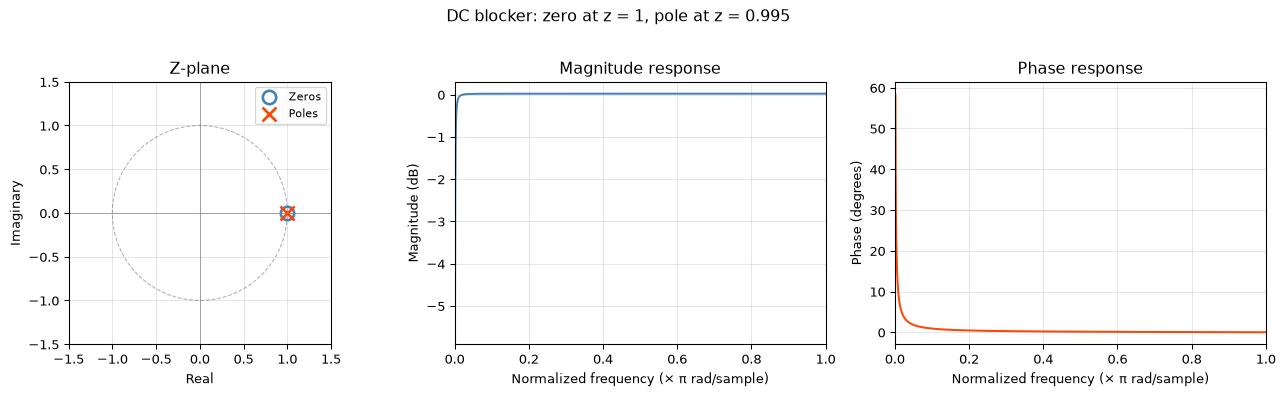
The explorer computes in the browser; here is the same thing in scipy.signal, which is where you would do reproducible work. Copy the b and a arrays from under the z-plane straight into this cell.
Static pole-zero plot in Python
import numpy as npimport matplotlib.pyplot as pltfrom scipy.signal import freqz, tf2zpk# DC blocker: H(z) = (1 - z^{-1}) / (1 - 0.995 z^{-1})b = [1, -1] # numerator coefficients (zero at z = 1)a = [1, -0.995] # denominator coefficients (pole at z = 0.995)z, p, k = tf2zpk(b, a)w, h = freqz(b, a, worN=1024)fig, axes = plt.subplots(1, 3, figsize=(14, 4))ax = axes[0]theta = np.linspace(0, 2* np.pi, 200)ax.plot(np.cos(theta), np.sin(theta), 'k--', alpha=0.3, linewidth=0.8)ax.plot(np.real(z), np.imag(z), 'o', markersize=10, markerfacecolor='none', markeredgecolor='steelblue', markeredgewidth=2, label='Zeros')ax.plot(np.real(p), np.imag(p), 'x', markersize=10, markeredgecolor='orangered', markeredgewidth=2, label='Poles')ax.axhline(0, color='grey', linewidth=0.5)ax.axvline(0, color='grey', linewidth=0.5)ax.set_xlim(-1.5, 1.5)ax.set_ylim(-1.5, 1.5)ax.set_aspect('equal')ax.set_xlabel('Real')ax.set_ylabel('Imaginary')ax.set_title('Z-plane')ax.legend(fontsize=8)ax.grid(True, alpha=0.3)ax = axes[1]ax.plot(w / np.pi, 20* np.log10(np.abs(h)), 'steelblue', linewidth=1.5)ax.set_xlabel('Normalized frequency (× π rad/sample)')ax.set_ylabel('Magnitude (dB)')ax.set_title('Magnitude response')ax.set_xlim(0, 1)ax.grid(True, alpha=0.3)ax = axes[2]ax.plot(w / np.pi, np.angle(h, deg=True), 'orangered', linewidth=1.5)ax.set_xlabel('Normalized frequency (× π rad/sample)')ax.set_ylabel('Phase (degrees)')ax.set_title('Phase response')ax.set_xlim(0, 1)ax.grid(True, alpha=0.3)fig.suptitle('DC blocker: zero at z = 1, pole at z = 0.995', fontsize=12, y=1.02)fig.tight_layout()plt.show()
/tmp/ipykernel_2893/4088053670.py:35: RuntimeWarning: divide by zero encountered in log10
  ax.plot(w / np.pi, 20 * np.log10(np.abs(h)), 'steelblue', linewidth=1.5)
tests/test_pole_zero_explorer.py keeps the two honest, with one caveat worth stating plainly: it reads the widget’s presets out of this page, reimplements its coefficient and response computation in Python, and checks that reimplementation against scipy.signal.freqz for every preset. What runs in your browser is the JavaScript, which no test executes. The port is short and deliberately line-for-line so the two can be diffed by eye, but the check is of the algorithm, not of the shipped code.
Prerequisites and next steps
This page assumes the z-domain (transfer functions, poles, zeros, the unit circle) and pairs with filter design, where specifications become pole and zero locations.
Source Code
---title: "Pole-Zero Explorer"subtitle: "Place, drag and delete poles and zeros; watch the frequency response follow"description-meta: "An interactive z-plane: place, drag and delete poles and zeros, and watch the frequency response follow."toc: falsealiases: - /topics/pole-zero-explorer/index.html---::: {.column-page}```{=html}<style>.pz { --pz-fg: #2b2b2b; --pz-mut: #6b7280; --pz-grid: rgba(0,0,0,0.09); --pz-axis: rgba(0,0,0,0.32); --pz-zero: #1f77b4; --pz-pole: #e2542c; --pz-cur: #7a4fbf; --pz-bd: rgba(0,0,0,0.14); --pz-panel: rgba(0,0,0,0.02); --pz-back: rgba(255,255,255,0.88); --pz-side: clamp(280px, 48vh, 470px); color: var(--pz-fg); margin-bottom: 1.2rem;}[data-bs-theme="dark"] .pz { --pz-fg: #e6e6e6; --pz-mut: #9aa3ad; --pz-grid: rgba(255,255,255,0.10); --pz-axis: rgba(255,255,255,0.34); --pz-zero: #5aa9e6; --pz-pole: #ff7a52; --pz-cur: #b79cff; --pz-bd: rgba(255,255,255,0.16); --pz-panel: rgba(255,255,255,0.035); --pz-back: rgba(34,34,34,0.88);}.pz-bar { display: flex; flex-wrap: wrap; align-items: center; gap: 0.35rem 0.9rem; padding: 0.45rem 0.6rem; margin-bottom: 0.6rem; border: 1px solid var(--pz-bd); border-radius: 6px; background: var(--pz-panel); font-size: 0.86rem;}.pz-grp { display: flex; align-items: center; gap: 0.3rem; }.pz-grp > .pz-lbl { color: var(--pz-mut); }.pz button { font: inherit; font-size: 0.84rem; line-height: 1.2; padding: 0.24rem 0.55rem; border: 1px solid var(--pz-bd); border-radius: 5px; background: transparent; color: inherit; cursor: pointer;}.pz button:hover { border-color: var(--pz-fg); }/* --pz-back, not --pz-panel: panel is a 2%-opaque wash meant to sit ON the page background, and as a foreground colour it is invisible against --pz-fg. */.pz button.is-on { background: var(--pz-fg); color: var(--pz-back); border-color: var(--pz-fg); }.pz-tool[data-tool="pole"].is-on { background: var(--pz-pole); border-color: var(--pz-pole); color: #fff; }.pz-tool[data-tool="zero"].is-on { background: var(--pz-zero); border-color: var(--pz-zero); color: #fff; }.pz-status { margin-left: auto; font-variant-numeric: tabular-nums; }.pz-status.bad { color: var(--pz-pole); font-weight: 600; }/* The z-plane is square, and its side also fixes the left column, so the hint and the coefficient box wrap under the plot instead of stretching the grid. */.pz-main { display: grid; grid-template-columns: var(--pz-side) minmax(320px, 1fr); gap: 0.5rem 1.1rem; align-items: start; }.pz-title { font-size: 0.78rem; letter-spacing: 0.04em; text-transform: uppercase; color: var(--pz-mut); margin: 0 0 0.15rem 0.1rem; }.pz-zwrap svg { height: var(--pz-side); width: var(--pz-side); display: block; touch-action: none; cursor: crosshair; }.pz-right svg { width: 100%; height: auto; display: block; touch-action: none; }.pz-right > div + div { margin-top: 0.35rem; }.pz-hint { font-size: 0.78rem; color: var(--pz-mut); margin-top: 0.3rem; }.pz-coef { font-family: var(--bs-font-monospace, monospace); font-size: 0.78rem; margin-top: 0.45rem; padding: 0.4rem 0.5rem; border: 1px solid var(--pz-bd); border-radius: 5px; background: var(--pz-panel); overflow-x: auto; white-space: nowrap;}@media (max-width: 820px) { .pz-main { grid-template-columns: 1fr; } .pz-zwrap svg { width: 100%; height: auto; }}</style><div class="pz" id="pz-app"> <div class="pz-bar"> <span class="pz-grp"> <span class="pz-lbl">click adds</span> <button class="pz-tool is-on" data-tool="pole" type="button">✕ pole pair</button> <button class="pz-tool" data-tool="zero" type="button">◯ zero pair</button> <button class="pz-tool" data-tool="erase" type="button">erase</button> </span> <span class="pz-grp"> <label><input type="checkbox" id="pz-snap" checked> snap to unit circle & real axis</label> </span> <span class="pz-grp"> <span class="pz-lbl">preset</span> <button data-preset="clear" type="button">empty</button> <button data-preset="dc" type="button">DC blocker</button> <button data-preset="lp" type="button">lowpass</button> <button data-preset="res" type="button">resonator</button> <button data-preset="notch" type="button">notch</button> <button data-preset="ap" type="button">allpass</button> </span> <span class="pz-status" id="pz-status"></span> </div> <div class="pz-main"> <div> <div class="pz-title">z-plane</div> <div class="pz-zwrap"> <!-- No role="img": this is not a static image. There is also no keyboard path to place or move a marker, which is a real gap, recorded in the project's verification notes rather than papered over with a role. --> <svg id="pz-zplane" viewBox="0 0 420 420" aria-label="Interactive z-plane. Click to place poles and zeros, drag to move them."></svg> </div> <div class="pz-hint">Click empty space to place · drag a marker to move it · right-click or Alt-click a marker to delete it. Off-axis markers are placed as conjugate pairs, so the coefficients stay real.</div> <div class="pz-coef" id="pz-coef"></div> </div> <div class="pz-right"> <div> <div class="pz-title">magnitude</div> <svg id="pz-mag" viewBox="0 0 560 215" role="img" aria-label="Magnitude response in decibels"></svg> </div> <div> <div class="pz-title">phase</div> <svg id="pz-pha" viewBox="0 0 560 190" role="img" aria-label="Phase response in degrees"></svg> </div> </div> </div></div><script>(function () { var app = document.getElementById("pz-app"); if (!app) return; var NS = "http://www.w3.org/2000/svg"; var R = 1.5; // z-plane half-domain: room for unstable poles // and for allpass zeros at 1.25, not much more var ZS = 420, ZP = 26; // z-plane viewBox size, padding var ZI = ZS - 2 * ZP; // inner span in viewBox units var NF = 600; // frequency samples on [0, pi] var MAX = 12; // cap on markers, keeps the state comprehensible var HIT = 13; // hit radius in viewBox units var FLOOR = 1e-12; // magnitude floor so a perfect null is finite in dB var zsvg = document.getElementById("pz-zplane"); var msvg = document.getElementById("pz-mag"); var psvg = document.getElementById("pz-pha"); var statusEl = document.getElementById("pz-status"); var coefEl = document.getElementById("pz-coef"); var snapEl = document.getElementById("pz-snap"); // Each item is one representative with im >= 0. A nonzero im implies its // conjugate, which is what keeps b and a real. var items = []; var tool = "pole"; var cursor = null; // normalized frequency under the pointer, 0..1 var markers = []; // rendered hit targets, rebuilt on every draw var resp = null; // cached frequency response function el(name, attrs, parent) { var n = document.createElementNS(NS, name), k; for (k in attrs) n.setAttribute(k, attrs[k]); if (parent) parent.appendChild(n); return n; } function wipe(n) { while (n.firstChild) n.removeChild(n.firstChild); } function txt(parent, x, y, s, attrs) { var a = { x: x, y: y, "font-size": 11, fill: "var(--pz-mut)" }, k; for (k in attrs) a[k] = attrs[k]; var t = el("text", a, parent); t.textContent = s; return t; } function fmt(v, n) { var s = v.toFixed(n); if (/\./.test(s)) s = s.replace(/0+$/, "").replace(/\.$/, ""); return s === "-0" ? "0" : s; } // z-plane <-> viewBox mapping function zx(re) { return ZP + (re + R) / (2 * R) * ZI; } function zy(im) { return ZP + (R - im) / (2 * R) * ZI; } function unzx(px) { return (px - ZP) / ZI * 2 * R - R; } function unzy(py) { return R - (py - ZP) / ZI * 2 * R; } function toSvg(svg, ev) { var m = svg.getScreenCTM(); if (!m) return { x: 0, y: 0 }; var p = new DOMPoint(ev.clientX, ev.clientY).matrixTransform(m.inverse()); return { x: p.x, y: p.y }; } // ---- model ------------------------------------------------------------- function expand(kind) { var out = [], i, it; for (i = 0; i < items.length; i++) { it = items[i]; if (it.t !== kind) continue; out.push({ re: it.re, im: it.im }); if (it.im > 1e-9) out.push({ re: it.re, im: -it.im }); } return out; } // H(z) = prod(1 - z_i z^-1) / prod(1 - p_i z^-1): the z^-1 convention, so the // polynomial coefficients below are exactly the b and a that scipy expects. function poly(kind) { var c = [1], i, it, f, j, out; for (i = 0; i < items.length; i++) { it = items[i]; if (it.t !== kind) continue; f = it.im > 1e-9 ? [1, -2 * it.re, it.re * it.re + it.im * it.im] : [1, -it.re]; out = new Array(c.length + f.length - 1); for (j = 0; j < out.length; j++) out[j] = 0; for (j = 0; j < c.length; j++) for (var k = 0; k < f.length; k++) out[j + k] += c[j] * f[k]; c = out; } return c; } function response() { var zs = expand("z"), ps = expand("p"); var mag = new Float64Array(NF + 1), pha = new Float64Array(NF + 1); for (var k = 0; k <= NF; k++) { var w = Math.PI * k / NF, cw = Math.cos(w), sw = Math.sin(w); var nr = 1, ni = 0, dr = 1, di = 0, i, q, fr, fi, tr; // e^{-jw} = cw - j sw, so 1 - q e^{-jw} has // real 1 - (q.re cw + q.im sw), imag q.re sw - q.im cw for (i = 0; i < zs.length; i++) { q = zs[i]; fr = 1 - (q.re * cw + q.im * sw); fi = q.re * sw - q.im * cw; tr = nr * fr - ni * fi; ni = nr * fi + ni * fr; nr = tr; } for (i = 0; i < ps.length; i++) { q = ps[i]; fr = 1 - (q.re * cw + q.im * sw); fi = q.re * sw - q.im * cw; tr = dr * fr - di * fi; di = dr * fi + di * fr; dr = tr; } var d2 = dr * dr + di * di; var hr, hi; if (d2 < 1e-300) { hr = 1e150; hi = 0; } else { hr = (nr * dr + ni * di) / d2; hi = (ni * dr - nr * di) / d2; } mag[k] = 20 * Math.log10(Math.max(Math.hypot(hr, hi), FLOOR)); pha[k] = Math.atan2(hi, hr) * 180 / Math.PI; } return { mag: mag, pha: pha }; } // ---- z-plane ----------------------------------------------------------- function drawStatic() { var g = el("g", { id: "pz-static" }, zsvg), i, v, c = []; for (i = -1; i <= 1.0001; i += 0.5) { if (Math.abs(i) < 1e-9) continue; el("line", { x1: zx(i), y1: ZP, x2: zx(i), y2: ZP + ZI, stroke: "var(--pz-grid)", "stroke-width": 1 }, g); el("line", { x1: ZP, y1: zy(i), x2: ZP + ZI, y2: zy(i), stroke: "var(--pz-grid)", "stroke-width": 1 }, g); } el("line", { x1: ZP, y1: zy(0), x2: ZP + ZI, y2: zy(0), stroke: "var(--pz-axis)", "stroke-width": 1 }, g); el("line", { x1: zx(0), y1: ZP, x2: zx(0), y2: ZP + ZI, stroke: "var(--pz-axis)", "stroke-width": 1 }, g); for (i = 0; i <= 240; i++) c.push((i ? "L" : "M") + zx(Math.cos(2 * Math.PI * i / 240)).toFixed(2) + " " + zy(Math.sin(2 * Math.PI * i / 240)).toFixed(2)); el("path", { d: c.join(" "), fill: "none", stroke: "var(--pz-axis)", "stroke-width": 1.2, "stroke-dasharray": "5 4" }, g); txt(g, ZP + ZI, zy(0) - 7, "Re", { "text-anchor": "end" }); txt(g, zx(0) + 6, ZP + 10, "Im"); // The circle is labelled by frequency rather than by ±1 and ±j: the angle is // the frequency, and a marker parked on ±1 would sit on top of the number. txt(g, zx(1.10), zy(0) - 7, "ω=0", { "text-anchor": "start", "font-size": 10 }); txt(g, zx(-1.10), zy(0) - 7, "ω=π", { "text-anchor": "end", "font-size": 10 }); txt(g, zx(0.07), zy(1.11), "ω=π/2", { "text-anchor": "start", "font-size": 10 }); el("g", { id: "pz-dyn" }, zsvg); el("g", { id: "pz-hover" }, zsvg); } function drawItems() { var g = zsvg.querySelector("#pz-dyn"); wipe(g); markers = []; for (var i = 0; i < items.length; i++) { var it = items[i]; place(g, it, i, false); if (it.im > 1e-9) place(g, it, i, true); } } function place(g, it, idx, mirror) { var im = mirror ? -it.im : it.im; var x = zx(it.re), y = zy(im); var r = Math.hypot(it.re, it.im); var col = it.t === "p" ? "var(--pz-pole)" : "var(--pz-zero)"; var bad = it.t === "p" && r >= 1; if (it.t === "p") { var s = 7; el("line", { x1: x - s, y1: y - s, x2: x + s, y2: y + s, stroke: col, "stroke-width": 2.4, "stroke-linecap": "round" }, g); el("line", { x1: x - s, y1: y + s, x2: x + s, y2: y - s, stroke: col, "stroke-width": 2.4, "stroke-linecap": "round" }, g); if (bad) el("circle", { cx: x, cy: y, r: 11, fill: "none", stroke: col, "stroke-width": 1, "stroke-dasharray": "2 2" }, g); } else { el("circle", { cx: x, cy: y, r: 7.5, fill: "none", stroke: col, "stroke-width": 2.4 }, g); } el("circle", { cx: x, cy: y, r: HIT, fill: "transparent", style: "cursor:grab" }, g); markers.push({ idx: idx, mirror: mirror, x: x, y: y }); // Coincident markers are a real configuration, not an accident: the lowpass // preset's double zero at z = -1 is the whole point of a Butterworth // numerator. Drawn plain they look like one marker, and the reader has no // way to tell why b = [1, 2, 1] instead of [1, 1]. Label the multiplicity. var mult = 0; for (var j = 0; j < items.length; j++) { var o = items[j]; if (o.t === it.t && Math.abs(o.re - it.re) < 1e-9 && Math.abs(o.im - it.im) < 1e-9) mult++; } if (mult > 1 && idx === firstIndexAt(it)) { txt(g, x + 11, y - 8, "×" + mult, { "font-size": 10.5, fill: col, "text-anchor": "start" }); } } function firstIndexAt(it) { for (var j = 0; j < items.length; j++) { var o = items[j]; if (o.t === it.t && Math.abs(o.re - it.re) < 1e-9 && Math.abs(o.im - it.im) < 1e-9) return j; } return -1; } function drawHover() { var g = zsvg.querySelector("#pz-hover"); wipe(g); if (cursor === null) return; var w = Math.PI * cursor, cx = zx(Math.cos(w)), cy = zy(Math.sin(w)); // Every distance from e^{jw} to a zero multiplies |H|; every distance to a // pole divides it. That is the whole geometric reading of the plot. for (var i = 0; i < markers.length; i++) { var m = markers[i], it = items[m.idx]; el("line", { x1: cx, y1: cy, x2: m.x, y2: m.y, stroke: it.t === "p" ? "var(--pz-pole)" : "var(--pz-zero)", "stroke-width": 1, "stroke-dasharray": "3 3", opacity: 0.65 }, g); } el("circle", { cx: cx, cy: cy, r: 5, fill: "var(--pz-cur)" }, g); } // ---- response plots ---------------------------------------------------- function niceStep(raw) { var steps = [1, 2, 5, 10, 20, 25, 50, 100, 200], i; for (i = 0; i < steps.length; i++) if (steps[i] >= raw) return steps[i]; return steps[steps.length - 1]; } // Both ends of the axis have to survive a singularity. A zero on the unit // circle sends one sample to the FLOOR (-240 dB); a POLE on the unit circle // sends one to +infinity, and ranging on the raw maximum then pushed the whole // curve off the top of the box -- at a pole snapped to z = 1, one sample of 601 // stayed inside the frame and the plot read as blank. So the top comes from a // high percentile plus a generous margin: wide enough that a genuine sharp // resonance (r = 0.999, +57 dB) is still framed whole, tight enough that a // divergence clips at the top edge, which is what a divergence should look like. function magRange() { var s = Array.prototype.slice.call(resp.mag).sort(function (a, b) { return a - b; }); var lo = s[0], hi = s[s.length - 1]; if (!isFinite(lo) || !isFinite(hi)) { lo = -20; hi = 20; } hi = Math.min(hi, s[Math.floor(0.98 * (s.length - 1))] + 40); lo = Math.max(lo, hi - 90); // a true null would run to -240 dB if (hi - lo < 8) { var mid = (hi + lo) / 2; lo = mid - 8; hi = mid + 8; } var step = niceStep((hi - lo) / 5); return { lo: Math.floor(lo / step) * step - step, hi: Math.ceil(hi / step) * step + step, step: step }; } function frame(svg, w, h, ml, mr, mt, mb, xTitle) { wipe(svg); var uid = svg.id + "-clip"; var defs = el("defs", {}, svg); var cp = el("clipPath", { id: uid }, defs); el("rect", { x: ml, y: mt, width: w - ml - mr, height: h - mt - mb }, cp); var g = el("g", {}, svg); el("rect", { x: ml, y: mt, width: w - ml - mr, height: h - mt - mb, fill: "none", stroke: "var(--pz-bd)", "stroke-width": 1 }, g); var px = function (f) { return ml + f * (w - ml - mr); }; for (var f = 0; f <= 1.0001; f += 0.25) { el("line", { x1: px(f), y1: mt, x2: px(f), y2: h - mb, stroke: "var(--pz-grid)", "stroke-width": 1 }, g); txt(g, px(f), h - mb + 13, fmt(f, 2), { "text-anchor": "middle", "font-size": 10 }); } if (xTitle) txt(g, (ml + w - mr) / 2, h - 3, xTitle, { "text-anchor": "middle", "font-size": 10.5 }); return { g: g, clip: "url(#" + uid + ")", px: px, ml: ml, mr: mr, mt: mt, mb: mb, w: w, h: h }; } function curve(fr, py, data, colour, breaks) { var d = [], k, prev = null, up = true; for (k = 0; k <= NF; k++) { if (breaks && prev !== null && Math.abs(data[k] - prev) > 180) up = true; d.push((up ? "M" : "L") + fr.px(k / NF).toFixed(2) + " " + py(data[k]).toFixed(2)); up = false; prev = data[k]; } el("path", { d: d.join(" "), fill: "none", stroke: colour, "stroke-width": 2, "clip-path": fr.clip, "stroke-linejoin": "round" }, fr.g); } function drawMag() { var W = 560, H = 215, fr = frame(msvg, W, H, 46, 10, 12, 24, null); var rg = magRange(); var py = function (v) { return fr.mt + (rg.hi - v) / (rg.hi - rg.lo) * (H - fr.mt - fr.mb); }; for (var v = rg.lo; v <= rg.hi + 1e-9; v += rg.step) { el("line", { x1: fr.ml, y1: py(v), x2: W - fr.mr, y2: py(v), stroke: Math.abs(v) < 1e-9 ? "var(--pz-axis)" : "var(--pz-grid)", "stroke-width": 1 }, fr.g); txt(fr.g, fr.ml - 6, py(v) + 3.5, fmt(v, 0), { "text-anchor": "end", "font-size": 10 }); } txt(fr.g, 11, (fr.mt + H - fr.mb) / 2, "dB", { "text-anchor": "middle", transform: "rotate(-90 11 " + ((fr.mt + H - fr.mb) / 2) + ")", "font-size": 10.5 }); curve(fr, py, resp.mag, "var(--pz-zero)", false); return { fr: fr, py: py }; } function drawPha() { var W = 560, H = 190, fr = frame(psvg, W, H, 46, 10, 12, 32, "normalized frequency ω/π (1 = Nyquist)"); var py = function (v) { return fr.mt + (180 - v) / 360 * (H - fr.mt - fr.mb); }; for (var v = -180; v <= 180; v += 90) { el("line", { x1: fr.ml, y1: py(v), x2: W - fr.mr, y2: py(v), stroke: v === 0 ? "var(--pz-axis)" : "var(--pz-grid)", "stroke-width": 1 }, fr.g); txt(fr.g, fr.ml - 6, py(v) + 3.5, String(v), { "text-anchor": "end", "font-size": 10 }); } txt(fr.g, 11, (fr.mt + H - fr.mb) / 2, "deg", { "text-anchor": "middle", transform: "rotate(-90 11 " + ((fr.mt + H - fr.mb) / 2) + ")", "font-size": 10.5 }); curve(fr, py, resp.pha, "var(--pz-pole)", true); return { fr: fr, py: py }; } function drawCursor(p, data, colour, label) { if (cursor === null) return; var k = Math.round(cursor * NF), x = p.fr.px(cursor), y = p.py(data[k]); el("line", { x1: x, y1: p.fr.mt, x2: x, y2: p.fr.h - p.fr.mb, stroke: "var(--pz-cur)", "stroke-width": 1 }, p.fr.g); el("circle", { cx: x, cy: y, r: 3.5, fill: "var(--pz-cur)", "clip-path": p.fr.clip }, p.fr.g); // A backing rect, because a tall resonance peak reaches this corner. var pad = 4, wid = label.length * 5.9 + 2 * pad; el("rect", { x: p.fr.w - p.fr.mr - 1 - wid, y: p.fr.mt + 1, width: wid, height: 17, fill: "var(--pz-back)", stroke: "none" }, p.fr.g); txt(p.fr.g, p.fr.w - p.fr.mr - 1 - pad, p.fr.mt + 13.5, label, { "text-anchor": "end", "font-size": 11, fill: "var(--pz-fg)" }); } // ---- glue -------------------------------------------------------------- function draw() { resp = response(); drawItems(); drawHover(); var m = drawMag(), p = drawPha(); if (cursor !== null) { var k = Math.round(cursor * NF); drawCursor(m, resp.mag, "var(--pz-zero)", "ω/π = " + cursor.toFixed(3) + " |H| = " + resp.mag[k].toFixed(2) + " dB"); drawCursor(p, resp.pha, "var(--pz-pole)", "∠H = " + resp.pha[k].toFixed(1) + "°"); } // Three states, matching the definition in basics/04-z-domain.qmd. A pole // exactly ON the circle is marginal, not unstable: its mode neither decays // nor grows, so calling it unstable would contradict the chapter this page // lists as its prerequisite. var worst = 0; for (var i = 0; i < items.length; i++) if (items[i].t === "p") worst = Math.max(worst, Math.hypot(items[i].re, items[i].im)); var marginal = Math.abs(worst - 1) < 1e-9; var unstable = worst > 1 + 1e-9; statusEl.textContent = items.length === 0 ? "no poles or zeros: H(z) = 1" : (unstable ? "UNSTABLE: pole at radius " + worst.toFixed(3) + ", outside the unit circle" : marginal ? "MARGINALLY STABLE: pole on the unit circle, mode neither decays nor grows" : "stable, largest pole radius " + (worst ? worst.toFixed(3) : "0")); statusEl.className = "pz-status" + (unstable || marginal ? " bad" : ""); var b = poly("z"), a = poly("p"); var show = function (v) { return v.map(function (x) { return fmt(x, 4); }).join(", "); }; coefEl.textContent = "b = [" + show(b) + "]\na = [" + show(a) + "]"; coefEl.style.whiteSpace = "pre"; } // ---- interaction ------------------------------------------------------- function snap(re, im) { if (snapEl.checked) { if (Math.abs(im) < 0.05) im = 0; var r = Math.hypot(re, im); if (r > 1e-6 && Math.abs(r - 1) < 0.045) { re /= r; im /= r; } } var lim = R - 0.06; re = Math.max(-lim, Math.min(lim, re)); im = Math.max(-lim, Math.min(lim, im)); return { re: re, im: im }; } // On a tie -- and coincident markers tie exactly -- a plain nearest-wins search // always returns the same one, so every other marker at that spot is // permanently unreachable. Remembering the last pick and skipping it makes // repeated clicks cycle through the stack instead. var lastPick = -1; function hit(x, y) { var within = [], i, m, d; for (i = 0; i < markers.length; i++) { m = markers[i]; d = (m.x - x) * (m.x - x) + (m.y - y) * (m.y - y); if (d <= HIT * HIT) within.push({ m: m, d: d }); } if (!within.length) return null; within.sort(function (a, b) { return a.d - b.d; }); var best = within[0]; if (within.length > 1 && best.m.idx === lastPick) { for (i = 1; i < within.length; i++) { if (Math.abs(within[i].d - best.d) < 1e-6) { best = within[i]; break; } } } lastPick = best.m.idx; return best.m; } var drag = null; zsvg.addEventListener("pointerdown", function (ev) { if (ev.button === 2) return; var p = toSvg(zsvg, ev), h = hit(p.x, p.y); if (h && (tool === "erase" || ev.altKey)) { items.splice(h.idx, 1); lastPick = -1; draw(); return; } if (h) { drag = { idx: h.idx, mirror: h.mirror }; // If capture is unavailable the drag must still end on pointerup, which is // why endDrag is also bound to window below. try { zsvg.setPointerCapture(ev.pointerId); } catch (e) { /* no capture */ } ev.preventDefault(); return; } if (tool === "erase") return; if (items.length >= MAX) { // MAX counts placements, not drawn markers: an off-axis placement draws two. statusEl.textContent = "limit of " + MAX + " placements reached, delete one first"; statusEl.className = "pz-status"; return; } var s = snap(unzx(p.x), unzy(p.y)); items.push({ t: tool === "pole" ? "p" : "z", re: s.re, im: Math.abs(s.im) }); draw(); }); zsvg.addEventListener("pointermove", function (ev) { if (!drag) return; var p = toSvg(zsvg, ev); var re = unzx(p.x), im = unzy(p.y); if (drag.mirror) im = -im; // the grabbed marker keeps the cursor var s = snap(re, im); if (s.im < 0) { s.im = -s.im; drag.mirror = !drag.mirror; } var it = items[drag.idx]; it.re = s.re; it.im = s.im; draw(); }); function endDrag(ev) { if (!drag) return; drag = null; try { if (zsvg.hasPointerCapture && zsvg.hasPointerCapture(ev.pointerId)) zsvg.releasePointerCapture(ev.pointerId); } catch (e) { /* capture was never taken */ } } zsvg.addEventListener("pointerup", endDrag); zsvg.addEventListener("pointercancel", endDrag); // Without capture the release can land on any element; a drag that never ends // leaves the marker glued to the bare cursor. window.addEventListener("pointerup", endDrag); zsvg.addEventListener("contextmenu", function (ev) { var p = toSvg(zsvg, ev), h = hit(p.x, p.y); if (!h) return; ev.preventDefault(); items.splice(h.idx, 1); draw(); }); function track(svg, ml, mr, w) { svg.addEventListener("pointermove", function (ev) { var p = toSvg(svg, ev); var f = (p.x - ml) / (w - ml - mr); cursor = Math.max(0, Math.min(1, f)); draw(); }); svg.addEventListener("pointerleave", function () { cursor = null; draw(); }); } track(msvg, 46, 10, 560); track(psvg, 46, 10, 560); app.querySelectorAll(".pz-tool").forEach(function (btn) { btn.addEventListener("click", function () { tool = btn.dataset.tool; app.querySelectorAll(".pz-tool").forEach(function (b) { b.classList.toggle("is-on", b === btn); }); }); }); // Every preset is exact, not eyeballed: the allpass radii are true // reciprocals (1/1.25 = 0.8), so its magnitude is flat to machine precision. var PRESETS = { clear: [], dc: [{ t: "z", re: 1, im: 0 }, { t: "p", re: 0.995, im: 0 }], lp: [{ t: "z", re: -1, im: 0 }, { t: "z", re: -1, im: 0 }, { t: "p", re: 0.7 * Math.cos(0.5), im: 0.7 * Math.sin(0.5) }], res: [{ t: "z", re: 1, im: 0 }, { t: "z", re: -1, im: 0 }, { t: "p", re: 0.97 * Math.cos(Math.PI / 4), im: 0.97 * Math.sin(Math.PI / 4) }], notch: [{ t: "z", re: Math.cos(Math.PI / 3), im: Math.sin(Math.PI / 3) }, { t: "p", re: 0.95 * Math.cos(Math.PI / 3), im: 0.95 * Math.sin(Math.PI / 3) }], ap: [{ t: "z", re: 1.25 * Math.cos(Math.PI / 3), im: 1.25 * Math.sin(Math.PI / 3) }, { t: "p", re: 0.8 * Math.cos(Math.PI / 3), im: 0.8 * Math.sin(Math.PI / 3) }] }; app.querySelectorAll("[data-preset]").forEach(function (btn) { btn.addEventListener("click", function () { items = PRESETS[btn.dataset.preset].map(function (o) { return { t: o.t, re: o.re, im: o.im }; }); draw(); }); }); snapEl.addEventListener("change", draw); drawStatic(); items = PRESETS.res.map(function (o) { return { t: o.t, re: o.re, im: o.im }; }); draw();})();</script>```:::## What you are looking atClick in the z-plane to place a pole pair or a zero pair, drag them around, and the magnitude and phase response follow. Hover a response plot to see where that frequency sits on the unit circle, and which distances produce the value there.The transfer function built from the markers is$$H(z) = \frac{\prod_i \left(1 - z_i z^{-1}\right)}{\prod_i \left(1 - p_i z^{-1}\right)},$$with $z_i$ the zeros and $p_i$ the poles. Writing it in $z^{-1}$ rather than $z$ matters: expanding the two products gives exactly the `b` and `a` coefficient arrays shown under the z-plane, the ones `scipy.signal.freqz(b, a)` and `lfilter(b, a, x)` take. The frequency response is this evaluated on the unit circle, $H(e^{j\omega})$, which is why the hover marker walks around that circle as you sweep the response plots.Because $|e^{-j\omega}| = 1$, each factor has magnitude $|1 - z_i e^{-j\omega}| = |e^{j\omega} - z_i|$: the distance from the frequency point on the unit circle to that zero. So$$\left|H(e^{j\omega})\right| = \frac{\prod_i \left|e^{j\omega} - z_i\right|}{\prod_i \left|e^{j\omega} - p_i\right|},$$which is what the dashed lines draw while you hover. Every distance to a zero multiplies the magnitude; every distance to a pole divides it. Drag a pole toward the circle and its distance shrinks toward zero at that angle, so the magnitude there blows up. Put a zero *on* the circle and one distance becomes exactly zero, so the magnitude does too.Off-axis markers are placed as conjugate pairs because real filter coefficients require it: a lone complex pole would give complex `b` or `a`. Markers snapped onto the real axis stand alone, which is the exception that proves the rule.## Guided explorations::: {.callout-important title="Turn snapping off for the radial ones"}Snapping is what makes a zero land *exactly* on the unit circle, so it is on by default. But it also means a marker within about 0.045 of the circle jumps back onto it, so a small radial nudge does nothing. Every exploration below that asks you to move a marker slightly in or out wants the **snap** checkbox cleared first.:::::: {.callout-tip title="Resonance sharpness"}Start from the **resonator** preset, clear **snap**, and drag the pole slowly outward along its radius. The peak narrows and grows as the pole approaches the unit circle, and the phase transition across it steepens at the same rate. This is the digital resonator, and it is also why a high-Q filter is numerically delicate: the response becomes hypersensitive to the pole's exact position, and therefore to coefficient rounding.:::::: {.callout-tip title="Notch depth"}With **snap** on, place a zero pair exactly on the unit circle and watch the magnitude plunge off the bottom of the axis: a true null. Now clear **snap** and drag it slightly inward or outward. The notch fills in immediately. Only zeros exactly on the circle produce genuine nulls, which is why finite coefficient precision limits how deep a real notch filter can go.:::::: {.callout-tip title="What a nearby pole does to a notch"}From the **notch** preset, clear **snap** and drag the pole toward its zero. The notch stays deep but gets narrower, because the pole cancels the zero's influence everywhere except very close to the null. This pole-near-zero trick is how narrow notch filters are built: the zero sets the depth, the pole sets the width. Take the pole all the way onto the zero and they cancel exactly: the response goes flat and the notch vanishes, which is the degenerate end of the same story.:::::: {.callout-tip title="Instability"}Drag a pole outside the unit circle. The status line flips to UNSTABLE and the marker gets a dashed ring. The magnitude plot still draws a curve, because $H(e^{j\omega})$ is defined there arithmetically, but for a causal filter it no longer means anything: the impulse response grows without bound and the actual output diverges. Reading a frequency response off an unstable pole-zero plot is a classic way to fool yourself.Stop *on* the circle on the way out and the status reads MARGINALLY STABLE instead. That is a third state, not a shade of unstable: the mode neither decays nor grows. The magnitude is genuinely infinite at that frequency, so the curve runs off the top of the plot rather than the axis rescaling to chase it.:::::: {.callout-tip title="Allpass"}The **allpass** preset puts a zero at radius $1.25$ and a pole at radius $0.8$ on the same ray, and $1/1.25 = 0.8$ exactly. The magnitude is flat: constant at $20\log_{10}(1/0.8^2) = 3.88$ dB, since the leading coefficient is fixed at $b_0 = 1$ rather than normalised. Only the phase moves.The flatness lives entirely in that pairing, $z_i = 1/\overline{p_i}$, and the widget does not enforce it: drag either marker on its own and the magnitude bulges immediately. Rotating the pole alone to $\omega = \pi/2$ while the zero stays put swings the response from $-5.7$ to $+12.2$ dB. Move *both*, keeping the same angle and reciprocal radii, and the response stays flat while the phase step slides in frequency. Breaking the pairing on purpose is worth doing once: it shows that "allpass" is a property of the arrangement, not of having a pole and a zero on the same ray. This is the mechanism behind allpass equalisers and fractional-delay filters.:::::: {.callout-tip title="Reading the coefficients"}Watch the `b` and `a` arrays while you drag. A conjugate pair at radius $r$ and angle $\theta$ contributes the quadratic factor $1 - 2r\cos\theta\, z^{-1} + r^2 z^{-2}$: this is the biquad section, seen from the z-plane. Placing two pairs and reading off the four coefficients is exactly what a filter design routine does for you.:::## Connection to filter designClassical filter design functions like `scipy.signal.butter`, `cheby1`, and `ellip` work by computing pole and zero locations that satisfy a given magnitude specification:- **Butterworth** places poles evenly on a circle in the s-plane, then maps them to the z-plane via the bilinear transform. For a lowpass design, all zeros end up at $z = -1$ (Nyquist). The result is a maximally flat passband.- **Chebyshev Type I** allows ripple in the passband, which lets the poles move onto an ellipse, achieving a sharper transition for the same filter order.- **Elliptic (Cauer)** adds zeros in the stopband too, producing equiripple in both passband and stopband. This gives the sharpest transition of any classical design for a given order.The explorer shows the fundamental mechanism underneath all of them: every feature in the frequency response, every peak, notch, and slope, traces back to a specific pole or zero in the z-plane.For the full treatment, see [Filter design](06-filter-design.qmd). For the theory the explorer sits on, see [The z-domain](04-z-domain.qmd), and for what happens when those coefficients meet finite arithmetic, [Filter structures](07-filter-structures.qmd).## Python equivalentThe explorer computes in the browser; here is the same thing in `scipy.signal`, which is where you would do reproducible work. Copy the `b` and `a` arrays from under the z-plane straight into this cell.```{python}#| code-fold: true#| code-summary: "Static pole-zero plot in Python"import numpy as npimport matplotlib.pyplot as pltfrom scipy.signal import freqz, tf2zpk# DC blocker: H(z) = (1 - z^{-1}) / (1 - 0.995 z^{-1})b = [1, -1] # numerator coefficients (zero at z = 1)a = [1, -0.995] # denominator coefficients (pole at z = 0.995)z, p, k = tf2zpk(b, a)w, h = freqz(b, a, worN=1024)fig, axes = plt.subplots(1, 3, figsize=(14, 4))ax = axes[0]theta = np.linspace(0, 2* np.pi, 200)ax.plot(np.cos(theta), np.sin(theta), 'k--', alpha=0.3, linewidth=0.8)ax.plot(np.real(z), np.imag(z), 'o', markersize=10, markerfacecolor='none', markeredgecolor='steelblue', markeredgewidth=2, label='Zeros')ax.plot(np.real(p), np.imag(p), 'x', markersize=10, markeredgecolor='orangered', markeredgewidth=2, label='Poles')ax.axhline(0, color='grey', linewidth=0.5)ax.axvline(0, color='grey', linewidth=0.5)ax.set_xlim(-1.5, 1.5)ax.set_ylim(-1.5, 1.5)ax.set_aspect('equal')ax.set_xlabel('Real')ax.set_ylabel('Imaginary')ax.set_title('Z-plane')ax.legend(fontsize=8)ax.grid(True, alpha=0.3)ax = axes[1]ax.plot(w / np.pi, 20* np.log10(np.abs(h)), 'steelblue', linewidth=1.5)ax.set_xlabel('Normalized frequency (× π rad/sample)')ax.set_ylabel('Magnitude (dB)')ax.set_title('Magnitude response')ax.set_xlim(0, 1)ax.grid(True, alpha=0.3)ax = axes[2]ax.plot(w / np.pi, np.angle(h, deg=True), 'orangered', linewidth=1.5)ax.set_xlabel('Normalized frequency (× π rad/sample)')ax.set_ylabel('Phase (degrees)')ax.set_title('Phase response')ax.set_xlim(0, 1)ax.grid(True, alpha=0.3)fig.suptitle('DC blocker: zero at z = 1, pole at z = 0.995', fontsize=12, y=1.02)fig.tight_layout()plt.show()````tests/test_pole_zero_explorer.py` keeps the two honest, with one caveat worth stating plainly: it reads the widget's presets out of this page, *reimplements* its coefficient and response computation in Python, and checks that reimplementation against `scipy.signal.freqz` for every preset. What runs in your browser is the JavaScript, which no test executes. The port is short and deliberately line-for-line so the two can be diffed by eye, but the check is of the algorithm, not of the shipped code.::: {.callout-note title="Prerequisites and next steps"}This page assumes [the z-domain](04-z-domain.qmd) (transfer functions, poles, zeros, the unit circle) and pairs with [filter design](06-filter-design.qmd), where specifications become pole and zero locations.:::