The theoretical 16-bit SNR is \(6.02 \times 16 + 1.76 = 98.1\) dB. But if the signal uses only the top 10 dB of the range, the signal amplitude is \(10^{-10/20} = 0.316\) of full scale. The signal power drops by 10 dB, but the quantization noise stays the same. Effective SNR = \(98.1 - 10 = 88.1\) dB.
Exercise 3: Averaging improvement
A temperature sensor has an SNR of 25 dB when reading a single sample.
How many samples must be averaged to achieve 40 dB SNR?
If the sensor is sampled at 100 Hz, how long does this take?
If the temperature changes on a timescale of 1 second, is this averaging strategy valid?
Solution
Need 15 dB improvement: \(K = 10^{15/10} = 31.6\), so 32 averages.
\(32 / 100 = 0.32\) seconds.
Yes, 0.32 seconds is well within the 1-second change timescale. The signal is approximately constant over the averaging window, so the assumption of identical signal in each measurement holds. If the required improvement were 40 dB (10,000 averages = 100 seconds), the answer would be no.
Exercise 4: Noise distributions
Gaussian noise with \(\sigma = 0.5\) V. What fraction of samples exceed \(\pm 1.5\) V in magnitude? (Hint: that’s \(3\sigma\).)
A 10-bit ADC with input range \(\pm 1\) V. What is the quantization step size \(Q\)? What is the variance of the quantization noise?
If you could choose between Gaussian noise with \(\sigma = 0.1\) and uniform noise with the same variance, which would be “safer” for a system with a hard clipping threshold at \(\pm 0.3\)?
Solution
The \(3\sigma\) rule: about 0.27% of Gaussian samples fall outside \(\pm 3\sigma\). So roughly 3 in 1000 samples will exceed \(\pm 1.5\) V.
Uniform is safer. With \(\sigma = 0.1\), the uniform distribution spans \([-W/2, W/2]\) where \(W = \sigma\sqrt{12} = 0.346\) V, so the maximum is \(\pm 0.173\) V, always within the \(\pm 0.3\) V threshold. Gaussian noise with \(\sigma = 0.1\) has a \(3\sigma\) range of \(\pm 0.3\) V, meaning about 0.3% of samples will clip. The Gaussian has unbounded tails; the uniform is strictly bounded.
Intermediate
Exercise 5: SNR estimation from data
Generate a noisy sinusoid and estimate the SNR using two methods.
Generate 2 seconds of a 50 Hz sinusoid (amplitude 1) at \(f_s = 1000\) Hz with additive Gaussian noise (\(\sigma = 0.3\)). Compute the true SNR.
Estimate the SNR by subtracting the known signal and measuring the residual power.
Estimate the SNR using only the noisy data: compute the power in the signal band (e.g., 45–55 Hz via FFT) and compare with the total noise power. How close is this to the true value?
Solution
import numpy as nprng = np.random.default_rng(42)fs =1000t = np.arange(2* fs) / fssignal = np.sin(2* np.pi *50* t)noise =0.3* rng.standard_normal(len(t))x = signal + noise# a) True SNRp_signal = np.mean(signal**2)p_noise = np.mean(noise**2)snr_true =10* np.log10(p_signal / p_noise)print(f"True SNR: {snr_true:.1f} dB")# b) Residual method (requires known signal)residual = x - signalp_residual = np.mean(residual**2)snr_residual =10* np.log10(p_signal / p_residual)print(f"Residual method: {snr_residual:.1f} dB")# c) FFT-based method (signal-blind)X = np.fft.rfft(x)freqs = np.fft.rfftfreq(len(x), 1/fs)power_spectrum = np.abs(X)**2/len(x)**2# Signal band: 45-55 Hzsignal_mask = (freqs >=45) & (freqs <=55)noise_mask =~signal_mask & (freqs >0)p_sig_fft = np.sum(power_spectrum[signal_mask])p_noise_fft = np.sum(power_spectrum[noise_mask])snr_fft =10* np.log10(p_sig_fft / p_noise_fft)print(f"FFT-based method: {snr_fft:.1f} dB")print("(Crude estimate: numerator includes noise in the signal band,")print(" denominator sums ~990 bins vs ~10, so this is a bandwidth-scaled ratio)")
True SNR: 7.4 dB
Residual method: 7.4 dB
FFT-based method: 7.5 dB
(Crude estimate: numerator includes noise in the signal band,
 denominator sums ~990 bins vs ~10, so this is a bandwidth-scaled ratio)
Exercise 6: Averaging: theory meets practice
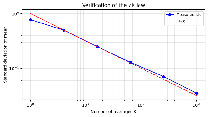
Verify the \(\sqrt{K}\) law experimentally.
Generate 10,000 samples of Gaussian noise (\(\sigma = 1\)). Add a constant signal of amplitude 0.1 (so the “signal” is just a DC offset buried in noise).
For \(K = 1, 4, 16, 64, 256, 1024\): take \(K\) consecutive samples, average them, and record the result. Repeat to get 100 such averages for each \(K\).
Plot the standard deviation of the 100 averages versus \(K\) on a log-log scale. Verify it follows \(\sigma / \sqrt{K}\).
Solution
import numpy as npimport matplotlib.pyplot as pltrng = np.random.default_rng(42)sigma =1.0dc_signal =0.1N =1024*100# enough for 100 blocks of max Kx = dc_signal + sigma * rng.standard_normal(N)K_values = [1, 4, 16, 64, 256, 1024]measured_std = []for K in K_values: n_blocks =100 block_means = [np.mean(x[i*K:(i+1)*K]) for i inrange(n_blocks)] measured_std.append(np.std(block_means))fig, ax = plt.subplots(figsize=(7, 4))ax.loglog(K_values, measured_std, 'bo-', markersize=6, label='Measured std')K_theory = np.array(K_values, dtype=float)ax.loglog(K_theory, sigma / np.sqrt(K_theory), 'r--', linewidth=1.5, label=r'$\sigma / \sqrt{K}$')ax.set_xlabel('Number of averages K')ax.set_ylabel('Standard deviation of mean')ax.legend(fontsize=9)ax.grid(True, alpha=0.3, which='both')ax.set_title('Verification of the √K law')fig.tight_layout()plt.show()
The measured standard deviation tracks the \(1/\sqrt{K}\) line closely, confirming that averaging independent noise samples reduces the standard deviation as predicted.
Exercise 7: Noise colour identification
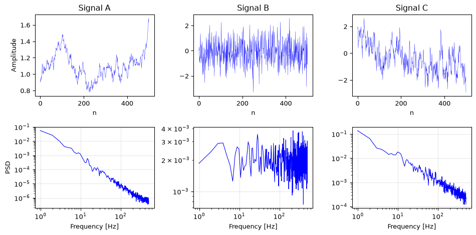
You are given three noise signals. Identify each as white, pink, or brown by examining the PSD.
Solution
import numpy as npimport matplotlib.pyplot as pltfrom scipy.signal import welchrng = np.random.default_rng(7)fs =1000N =8192# Generate the three noise types (shuffled)white = rng.standard_normal(N)freqs_fft = np.fft.rfftfreq(N, 1/fs)freqs_fft[0] =1W = np.fft.rfft(rng.standard_normal(N))pink = np.fft.irfft(W / np.sqrt(freqs_fft), N)brown = np.cumsum(rng.standard_normal(N))brown -= np.mean(brown)# Present in shuffled ordersignals = [('Signal A', brown), ('Signal B', white), ('Signal C', pink)]fig, axes = plt.subplots(2, 3, figsize=(10, 5))for i, (name, s) inenumerate(signals): s = s / np.std(s) # normalise for fair display axes[0, i].plot(s[:500], 'b-', linewidth=0.3) axes[0, i].set_title(name) axes[0, i].set_xlabel('n') f, psd = welch(s, fs, nperseg=1024) axes[1, i].loglog(f[1:], psd[1:], 'b-', linewidth=0.8) axes[1, i].set_xlabel('Frequency [Hz]') axes[1, i].grid(True, alpha=0.3)axes[0, 0].set_ylabel('Amplitude')axes[1, 0].set_ylabel('PSD')fig.tight_layout()plt.show()print("Signal A: PSD falls as 1/f² → Brown noise")print("Signal B: PSD is flat → White noise")print("Signal C: PSD falls as 1/f → Pink noise")
Signal A: PSD falls as 1/f² → Brown noise
Signal B: PSD is flat → White noise
Signal C: PSD falls as 1/f → Pink noise
The key diagnostic is the PSD slope on a log-log plot: flat = white, \(-1\) slope = pink, \(-2\) slope = brown.
Challenge
Exercise 8: Filtering improves SNR (quantitative)
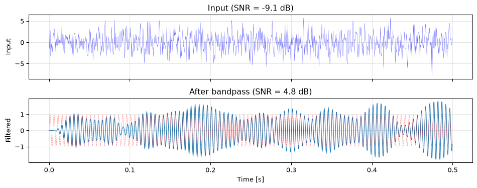
A 200 Hz sinusoid is buried in white noise. The sampling rate is \(f_s = 2000\) Hz.
Generate the signal (amplitude 1) with noise (\(\sigma = 2\), so SNR \(\approx -9\) dB, the signal is weaker than the noise). Verify the SNR.
Design a bandpass filter (180–220 Hz passband) and apply it. What is the output SNR?
Compute the theoretical SNR improvement: the noise bandwidth goes from \(f_s/2 = 1000\) Hz to 40 Hz. How does this compare with the measured improvement?
Input SNR: -9.1 dB
Output SNR: 4.8 dB
Improvement: 13.9 dB
Theoretical improvement: 14.0 dB
The measured improvement is close to the theoretical \(10\log_{10}(1000/40) = 14\) dB. The small difference is because the Butterworth filter’s passband is not a perfect rectangle; it has a gradual roll-off, so the effective noise bandwidth is slightly wider than 40 Hz.
Exercise 9: The ENOB trap
The effective number of bits (ENOB) is the number of bits an ideal ADC would need to achieve the same SNR as a real one:
A 12-bit ADC datasheet claims 72 dB SNR. What is the ENOB? How many bits are “lost” to non-idealities?
Generate a full-scale sinusoid, quantize it with an ideal 12-bit quantizer, then add 0.5 LSB of Gaussian noise (simulating analog front-end noise). Measure the SNR and ENOB.
Now add 5% gain error (multiply the signal by 1.05 before quantizing). How does this affect ENOB?
Solution
\(\text{ENOB} = (72 - 1.76) / 6.02 = 11.67\) bits. The ADC loses \(12 - 11.67 = 0.33\) bits to non-idealities (INL, DNL, clock jitter, etc.). This is a good result: losing less than half a bit is typical for a quality ADC.
b) SNR = 68.0 dB, ENOB = 11.00 bits (lost 1.00 bits)
c) SNR = 27.3 dB, ENOB = 4.24 bits (lost 7.76 bits)
   Gain error costs 6.76 bits of ENOB
The analog front-end noise costs a fraction of a bit. The gain error may cost less or more depending on its magnitude, but the key insight is that ENOB is always less than the advertised bit count, and the gap tells you how much performance your analog chain is giving away.
Basic (continued)
Exercise 10: Debug this: broken dB conversion (Basic)
A student wrote this function to convert a power ratio to decibels and to check whether two SNR values differ by more than 3 dB:
import numpy as npdef power_to_db(ratio):return20* np.log10(ratio) # line Adef snr_improved_enough(snr1_db, snr2_db, threshold=3.0):return (snr2_db - snr1_db) > threshold # line Bratio =2.0print(f"{ratio}× power ratio = {power_to_db(ratio):.2f} dB")snr_before =10* np.log10(50)snr_after =10* np.log10(100)print(f"Improved enough? {snr_improved_enough(snr_before, snr_after)}")
Identify the bug on line A. What number does it currently print, and what should it print?
Line B is logically correct but will it give the right answer with the bug on line A present? Explain.
Fix line A and verify both outputs are correct.
Solution
Line A uses the amplitude formula (20 log₁₀) instead of the power formula (10 log₁₀). A power ratio of 2 should be \(10\log_{10}(2) = 3.01\) dB, but the bug prints \(20\log_{10}(2) = 6.02\) dB.
Line B compares two values both computed with 10 log₁₀ (the snr_before/snr_after variables are calculated correctly separately). The bug is only in power_to_db, so line B gives the right answer here, but if anyone calls snr_improved_enough with values produced by the buggy power_to_db, the threshold comparison will be wrong because the dB values will be twice as large as they should be.
Fix: replace 20 * np.log10 with 10 * np.log10 on line A.
import numpy as npdef power_to_db(ratio):return10* np.log10(ratio) # fixed: power ratio uses factor 10def snr_improved_enough(snr1_db, snr2_db, threshold=3.0):return (snr2_db - snr1_db) > thresholdratio =2.0print(f"{ratio}× power ratio = {power_to_db(ratio):.2f} dB") # expect 3.01 dBsnr_before =10* np.log10(50)snr_after =10* np.log10(100)print(f"Improved enough? {snr_improved_enough(snr_before, snr_after)}") # expect True (3.01 dB gain)
2.0× power ratio = 3.01 dB
Improved enough? True
The mnemonic: power uses 10, amplitude/voltage uses 20. Since power ∝ amplitude², \(20\log_{10}(A) = 10\log_{10}(A^2) = 10\log_{10}(P)\), the factor of 2 moves inside the log.
Exercise 11: Noise source budget (Basic)
A sensor circuit has three independent noise sources:
Source
Type
RMS level
Resistor thermal noise
White
12 µV
ADC quantization noise
White
8 µV
Power supply ripple
Narrowband (~50 Hz)
5 µV
Compute the total RMS noise. (Independent noise sources add in quadrature: \(\sigma_\text{total} = \sqrt{\sigma_1^2 + \sigma_2^2 + \sigma_3^2}\).)
The signal amplitude is 1 mV (peak), giving an RMS of \(1/\sqrt{2}\) mV. What is the SNR in dB?
If you could eliminate one noise source, which would give the largest SNR improvement?
The system specification requires 40 dB SNR. Is the current design within spec?
Solution
import numpy as npsigma_thermal =12e-6# V RMSsigma_adc =8e-6sigma_ripple =5e-6sigma_total = np.sqrt(sigma_thermal**2+ sigma_adc**2+ sigma_ripple**2)print(f"Total RMS noise: {sigma_total*1e6:.2f} µV")signal_rms =1e-3/ np.sqrt(2)snr =10* np.log10(signal_rms**2/ sigma_total**2)print(f"SNR: {snr:.1f} dB")# c) Impact of removing each sourcefor name, val in [("thermal", sigma_thermal), ("ADC", sigma_adc), ("ripple", sigma_ripple)]: sigma_without = np.sqrt(sigma_total**2- val**2) snr_without =10* np.log10(signal_rms**2/ sigma_without**2)print(f" Remove {name}: SNR = {snr_without:.1f} dB (gain = {snr_without - snr:.1f} dB)")print(f"\nd) Spec requires 40 dB. Current SNR = {snr:.1f} dB → {'PASS'if snr >=40else'FAIL'}")
Total RMS noise: 15.26 µV
SNR: 33.3 dB
  Remove thermal: SNR = 37.5 dB (gain = 4.2 dB)
  Remove ADC: SNR = 34.7 dB (gain = 1.4 dB)
  Remove ripple: SNR = 33.8 dB (gain = 0.5 dB)

d) Spec requires 40 dB. Current SNR = 33.3 dB → FAIL
The thermal noise dominates because it contributes most to the quadrature sum. Reducing the dominant source (thermal noise) gives the largest improvement; reducing a smaller contributor like ADC noise has diminishing returns in a quadrature sum. The ripple contribution is smallest, but unlike white noise, it is coherent and appears as a tone, which may cause different problems (interference, intermodulation) beyond what the RMS budget captures.
Exercise 12: Is this noise Gaussian? (Basic)
You are given a 5000-sample noise recording. Your task is to check whether it is plausibly Gaussian.
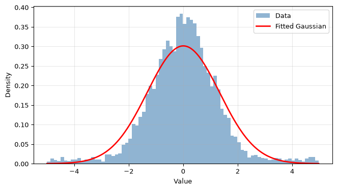
Generate the data: mix 90% Gaussian noise (\(\sigma = 1\)) with 10% uniform noise on \([-5, 5]\) (this simulates occasional interference spikes). Use rng = np.random.default_rng(99).
Compute the sample mean, variance, skewness, and kurtosis. For a true Gaussian, skewness = 0 and excess kurtosis = 0.
Plot a histogram with a fitted Gaussian overlay. Does the distribution look Gaussian by eye?
Based on the statistics, would you say this noise is close enough to Gaussian to use in a system designed for Gaussian noise assumptions?
Mean:            0.0075  (expect ≈ 0)
Variance:        1.7535  (expect ≈ 1.7 for this 90/10 Gaussian+uniform mix)
Skewness:        0.0383  (expect ≈ 0)
Excess kurtosis: 2.0567  (expect ≈ 0 for Gaussian, positive for heavy-tailed mix)
The excess kurtosis is positive (leptokurtic): the tails are heavier than Gaussian because the 10% uniform component on \([-5, 5]\) injects samples far from the mean (the uniform has \(\sigma \approx 2.9\), much wider than the Gaussian \(\sigma = 1\)). By eye the histogram shows slightly heavier flanks and a flatter peak than a pure Gaussian. Whether “close enough” depends on the application: for SNR calculations the difference is modest, but for rare-event probabilities (e.g. bit error rate) the tail shape matters a lot.
A student tries to verify the \(\sqrt{K}\) averaging law but their measured improvement is consistently about 1.5 dB less than expected. Find the bug.
import numpy as nprng = np.random.default_rng(0)sigma =1.0N =10000noise = rng.standard_normal(N)K_values = [4, 16, 64, 256]for K in K_values: n_blocks = N // K block_means = []for i inrange(n_blocks): block = noise[i*K : i*K + K +1] # <-- suspect line block_means.append(np.mean(block)) measured_std = np.std(block_means) expected_std = sigma / np.sqrt(K) improvement =10* np.log10(sigma**2/ measured_std**2) expected_db =10* np.log10(K)print(f"K={K:3d}: measured {improvement:.1f} dB, expected {expected_db:.1f} dB")
What does the slice noise[i*K : i*K + K + 1] actually return? How many samples does it include?
How does this affect the averaging? Why does it cause an underestimate of the improvement?
Fix the bug and re-run to confirm the measurements match theory.
Solution
The slice noise[i*K : i*K + K + 1] returns K + 1 samples instead of K. Python’s slice a:b returns indices a, a+1, ..., b-1, so a : a + K + 1 gives K + 1 elements. Each “block” is one sample longer than intended.
Two effects combine. First, each block has K + 1 samples, so the actual noise reduction is \(10\log_{10}(K+1)\), slightly more than the expected \(10\log_{10}(K)\). Second, and more importantly, consecutive blocks overlap by one sample (block \(i\) ends at index i*K + K, block \(i+1\) starts at (i+1)*K = i*K + K). This shared sample introduces positive correlation between adjacent block means. Correlated block means have higher variance than independent ones, so np.std(block_means) is inflated, which makes the measured noise reduction appear smaller than theory predicts. The overlap effect dominates, producing the observed ~1.5 dB shortfall.
import numpy as nprng = np.random.default_rng(0)sigma =1.0N =10000noise = rng.standard_normal(N)K_values = [4, 16, 64, 256]print("Fixed version:")for K in K_values: n_blocks = N // K block_means = []for i inrange(n_blocks): block = noise[i*K : i*K + K] # fixed: K samples, not K+1 block_means.append(np.mean(block)) measured_std = np.std(block_means) improvement =10* np.log10(sigma**2/ measured_std**2) expected_db =10* np.log10(K)print(f"K={K:3d}: measured {improvement:.1f} dB, expected {expected_db:.1f} dB")
Fixed version:
K=  4: measured 5.9 dB, expected 6.0 dB
K= 16: measured 11.8 dB, expected 12.0 dB
K= 64: measured 16.6 dB, expected 18.1 dB
K=256: measured 25.2 dB, expected 24.1 dB
Fix: remove the + 1 from the upper slice bound. The corrected results track \(10\log_{10}(K)\) closely.
Exercise 14: Estimate noise statistics from data (Intermediate)
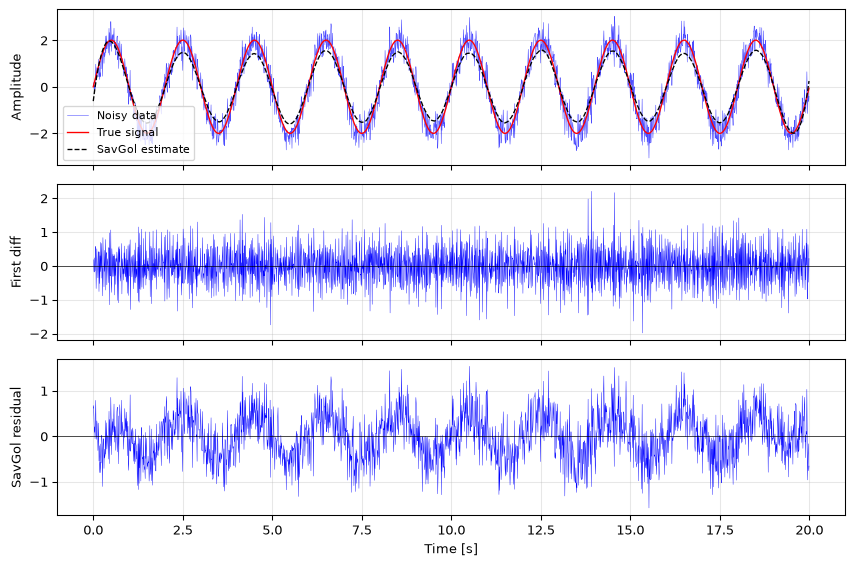
You receive a recording that contains a slowly varying signal plus noise. Your task is to estimate the noise standard deviation without knowing the true signal.
Generate the data: a low-frequency sinusoid (0.5 Hz, amplitude 2) sampled at 100 Hz for 20 seconds, plus Gaussian noise (\(\sigma = 0.4\)). Use rng = np.random.default_rng(7).
A simple approach: take first differences \(d[n] = x[n] - x[n-1]\). For a slowly varying signal, the signal component in \(d[n]\) is small compared to the noise component. Estimate \(\sigma_\text{noise}\) from \(\text{std}(d) / \sqrt{2}\) and compare with the true value.
A better approach: fit and subtract a smoothed estimate of the signal (use scipy.signal.savgol_filter with a long window), then estimate \(\sigma\) from the residual. Compare with the true value.
Which method is more accurate here, and why does the first-difference method have a factor of \(\sqrt{2}\)?
Solution
import numpy as npimport matplotlib.pyplot as pltfrom scipy.signal import savgol_filterrng = np.random.default_rng(7)fs =100t = np.arange(20* fs) / fssignal =2* np.sin(2* np.pi *0.5* t)noise =0.4* rng.standard_normal(len(t))x = signal + noisetrue_sigma =0.4# b) First-difference methodd = np.diff(x)sigma_diff = np.std(d) / np.sqrt(2)print(f"True sigma: {true_sigma:.4f}")print(f"First-difference method: {sigma_diff:.4f} (error {abs(sigma_diff-true_sigma)/true_sigma*100:.1f}%)")# c) Savitzky-Golay smoothing then residual# Window 201 samples = 2 s — long enough to track the 2 s period sinusoidsmoothed = savgol_filter(x, window_length=201, polyorder=3)residual = x - smoothedsigma_savgol = np.std(residual)print(f"Savitzky-Golay residual: {sigma_savgol:.4f} (error {abs(sigma_savgol-true_sigma)/true_sigma*100:.1f}%)")fig, axes = plt.subplots(3, 1, figsize=(9, 6), sharex=True)axes[0].plot(t, x, 'b-', linewidth=0.4, alpha=0.7, label='Noisy data')axes[0].plot(t, signal, 'r-', linewidth=1, label='True signal')axes[0].plot(t, smoothed, 'k--', linewidth=1, label='SavGol estimate')axes[0].legend(fontsize=8); axes[0].set_ylabel('Amplitude')axes[1].plot(t[1:], d, 'b-', linewidth=0.3)axes[1].set_ylabel('First diff'); axes[1].axhline(0, color='k', linewidth=0.5)axes[2].plot(t, residual, 'b-', linewidth=0.3)axes[2].set_ylabel('SavGol residual'); axes[2].axhline(0, color='k', linewidth=0.5)axes[2].set_xlabel('Time [s]')for ax in axes: ax.grid(True, alpha=0.3)fig.tight_layout()plt.show()
The Savitzky-Golay residual method is more accurate because it models the signal shape directly. The first-difference method works because \(d[n] = (s[n]-s[n-1]) + (w[n]-w[n-1])\); if the signal varies slowly the signal term is small and \(d[n] \approx w[n] - w[n-1]\). Since \(\text{Var}(w[n]-w[n-1]) = 2\sigma^2\) for independent noise, dividing by \(\sqrt{2}\) recovers \(\sigma\). However, for a 0.5 Hz sinusoid sampled at 100 Hz the signal step per sample is not negligible, so the first-difference estimate has residual signal contamination.
Exercise 15: How many bits do I need? (Intermediate)
Engineering judgement exercise: for each scenario decide the minimum ADC resolution (bits) and justify your answer.
A digital audio recording system. The listening environment adds a noise floor equivalent to 30 dB SPL; the maximum undistorted level is 100 dB SPL, giving an effective dynamic range of 70 dB.
A weighing scale. The maximum weight is 10 kg; the required resolution is 1 g.
A gyroscope for a drone flight controller. Full-scale range ±2000 °/s; required resolution 0.05 °/s. The update rate is 1 kHz and oversampling by factor 16 is possible.
A 12-bit ADC costs €2. A 16-bit ADC costs €8. Your audio application needs 80 dB SNR. Budget is tight. Which do you buy, and why?
Solution
import numpy as npdef bits_for_snr(snr_db):"""Minimum bits from quantization SNR formula."""return np.ceil((snr_db -1.76) /6.02)# a) Audio# Dynamic range needed: 100 - 30 = 70 dB. Industry standard is 96 dB (16-bit).snr_audio =70bits_audio = bits_for_snr(snr_audio)print(f"a) Audio: need {snr_audio} dB → {bits_audio:.0f} bits minimum")print(f" 16-bit gives {6.02*16+1.76:.0f} dB. Industry uses 24-bit for headroom.")# b) Scale: 10 kg / 0.001 kg = 10000 levels neededratio_scale =10/0.001bits_scale = np.ceil(np.log2(ratio_scale))snr_scale =6.02* bits_scale +1.76print(f"\nb) Scale: need {ratio_scale:.0f} levels → {bits_scale:.0f} bits ({snr_scale:.0f} dB)")# c) Gyroscope with oversamplingfull_range =4000# ±2000 °/s → 4000 °/s totalrequired_res =0.05levels = full_range / required_resbits_no_os = np.ceil(np.log2(levels))oversampling =16bits_saved = np.log2(oversampling) /2# each 4× oversampling adds 1 bitbits_with_os = bits_no_os - bits_savedprint(f"\nc) Gyro: {levels:.0f} levels → {bits_no_os:.0f} bits without OS")print(f" 16× oversampling adds {bits_saved:.1f} bits → need {bits_with_os:.0f} bits ADC")# d) Budget decisionsnr_target =80bits_needed = bits_for_snr(snr_target)snr_12bit =6.02*12+1.76snr_16bit =6.02*16+1.76print(f"\nd) Need {snr_target} dB → {bits_needed:.0f} bits minimum")print(f" 12-bit: {snr_12bit:.0f} dB (below target by {snr_target - snr_12bit:.0f} dB)")print(f" 16-bit: {snr_16bit:.0f} dB (headroom {snr_16bit - snr_target:.0f} dB)")
a) Audio: need 70 dB → 12 bits minimum
   16-bit gives 98 dB. Industry uses 24-bit for headroom.

b) Scale: need 10000 levels → 14 bits (86 dB)

c) Gyro: 80000 levels → 17 bits without OS
   16× oversampling adds 2.0 bits → need 15 bits ADC

d) Need 80 dB → 13 bits minimum
   12-bit: 74 dB (below target by 6 dB)
   16-bit: 98 dB (headroom 18 dB)
Answers:
12 bits gives 74 dB, which covers the 70 dB range. In practice, audio uses 16-bit (96 dB) or 24-bit for studio headroom.
14 bits (16384 levels covers the 10000 required).
Without oversampling: 17 bits. With 16× oversampling and decimation, the ADC gains 2 effective bits, so a 15-bit ADC suffices. In practice a 16-bit IMU part is used for margin.
The 12-bit ADC gives 74 dB, not enough for 80 dB. Buy the 16-bit for €8. The €6 premium buys 18 dB of headroom over the 80 dB target and compliance with the specification. A cheaper alternative: check if the sensor’s analog noise already limits you below 12-bit; if so, a more careful analog design might let the 12-bit work, saving €6 and avoiding a PCB respin.
Challenge (continued)
Exercise 16: White or colored? Decide from data (Challenge)
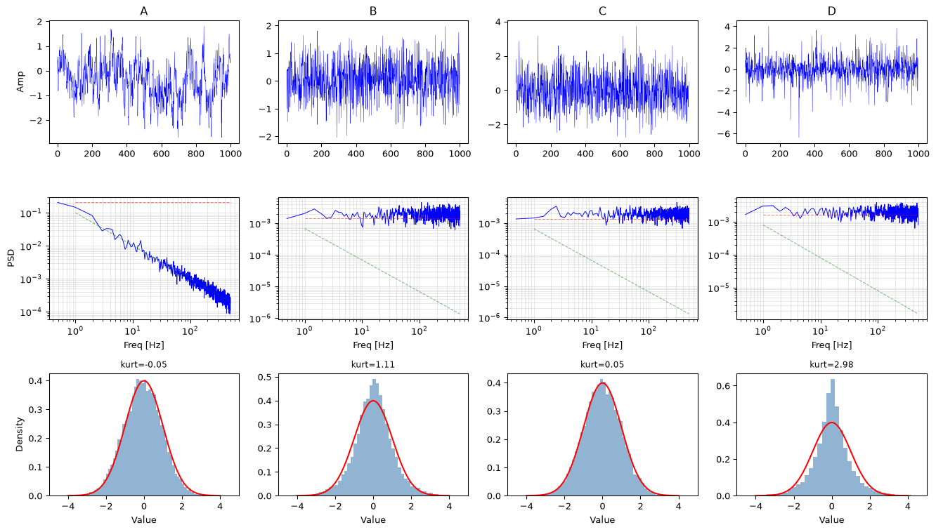
You receive four unlabelled noise time series. For each one, determine: (1) whether it is white, pink, or brown; (2) whether it is stationary; (3) whether it is approximately Gaussian.
Use only the data, no peeking at the generation code until after you have formed a hypothesis.
Solution
import numpy as npimport matplotlib.pyplot as pltfrom scipy.signal import welchfrom scipy import statsrng = np.random.default_rng(42)fs =1000N =16384# --- Generate the four signals (hidden from students) ---# A: pink noise (1/f)f_fft = np.fft.rfftfreq(N, 1/fs); f_fft[0] =1W = np.fft.rfft(rng.standard_normal(N))A = np.real(np.fft.irfft(W / np.sqrt(f_fft), N))# B: white noise, non-stationary (variance doubles halfway)B = np.concatenate([rng.standard_normal(N//2), 2* rng.standard_normal(N//2)])# C: white GaussianC = rng.standard_normal(N)# D: Laplacian (white but non-Gaussian — heavier tails)D = rng.laplace(0, 1/np.sqrt(2), N) # var=1 like Csignals = [('A', A), ('B', B), ('C', C), ('D', D)]fig, axes = plt.subplots(3, 4, figsize=(14, 8))for col, (name, s) inenumerate(signals): s_norm = s / np.std(s)# Time series axes[0, col].plot(s_norm[:1000], 'b-', linewidth=0.3) axes[0, col].set_title(name); axes[0, col].set_ylabel('Amp'if col ==0else'')# PSD f, psd = welch(s_norm, fs, nperseg=2048) axes[1, col].loglog(f[1:], psd[1:], 'b-', linewidth=0.7) axes[1, col].set_xlabel('Freq [Hz]') axes[1, col].set_ylabel('PSD'if col ==0else'') axes[1, col].grid(True, alpha=0.3, which='both')# Reference slopes f_ref = np.array([1, 500]) axes[1, col].loglog(f_ref, psd[1] * (f_ref / f[1])**0, 'r--', linewidth=0.8, alpha=0.5) axes[1, col].loglog(f_ref, psd[1] * (f_ref / f[1])**-1, 'g--', linewidth=0.8, alpha=0.5)# Histogram axes[2, col].hist(s_norm, bins=60, density=True, color='steelblue', alpha=0.6) x_g = np.linspace(-4, 4, 200) axes[2, col].plot(x_g, stats.norm.pdf(x_g), 'r-', linewidth=1.5) axes[2, col].set_xlim(-5, 5) axes[2, col].set_xlabel('Value') axes[2, col].set_ylabel('Density'if col ==0else'')# Kurtosis annotation k = stats.kurtosis(s_norm) axes[2, col].set_title(f'kurt={k:.2f}', fontsize=9)fig.tight_layout()plt.show()print("Answers:")print("A — Pink (PSD slope ≈ -1 on log-log). Stationary. Approx Gaussian (kurtosis ≈ 0).")print("B — White (flat PSD). Non-stationary: variance doubles at N/2 (visible in time plot).")print(" Running-variance test or split-half std comparison would confirm.")print("C — White. Stationary. Gaussian.")print("D — White (flat PSD). Stationary. Non-Gaussian: Laplacian has excess kurtosis ≈ 3,")print(" visible as a sharper peak and heavier tails than the Gaussian overlay.")# Numerical confirmationfor name, s in signals: half =len(s) //2print(f"{name}: kurtosis={stats.kurtosis(s):.2f} "f"std_1st={np.std(s[:half]):.3f} std_2nd={np.std(s[half:]):.3f}")
Answers:
A — Pink (PSD slope ≈ -1 on log-log). Stationary. Approx Gaussian (kurtosis ≈ 0).
B — White (flat PSD). Non-stationary: variance doubles at N/2 (visible in time plot).
   Running-variance test or split-half std comparison would confirm.
C — White. Stationary. Gaussian.
D — White (flat PSD). Stationary. Non-Gaussian: Laplacian has excess kurtosis ≈ 3,
   visible as a sharper peak and heavier tails than the Gaussian overlay.
A: kurtosis=-0.05  std_1st=0.146  std_2nd=0.133
B: kurtosis=1.11  std_1st=0.999  std_2nd=2.025
C: kurtosis=0.05  std_1st=1.002  std_2nd=0.993
D: kurtosis=2.98  std_1st=0.998  std_2nd=0.995
Diagnostic checklist:
Test
Detects
PSD slope on log-log
Noise colour (0=white, −1=pink, −2=brown)
Split-half variance ratio
Non-stationarity
Excess kurtosis
Heavy/light tails vs Gaussian
Time-series eye inspection
Slow drift, bursts, obvious non-stationarity
Signal D is the trap: it is spectrally white (passes PSD tests) but has non-Gaussian amplitude statistics, which matters for outlier detection and any method that assumes Gaussianity.
A student writes a function to measure the SNR improvement from averaging, but the numbers do not match theory. The function returns the same improvement for all K values.
import numpy as npdef measure_snr_improvement(K, n_trials=200, seed=0): rng = np.random.default_rng(seed) signal_power =0.5# constant DC signal, power = amplitude² noise_sigma =1.0 snr_single_db =10* np.log10(signal_power / noise_sigma**2) improvements = []for _ inrange(n_trials): samples = rng.standard_normal(K) + np.sqrt(signal_power) averaged = np.mean(samples) snr_avg =10* np.log10(averaged**2/ noise_sigma**2) # line X improvements.append(snr_avg - snr_single_db)return np.mean(improvements)for K in [4, 16, 64, 256]: measured = measure_snr_improvement(K) expected =10* np.log10(K)print(f"K={K:3d}: measured={measured:.1f} dB expected={expected:.1f} dB")
On line X, noise_sigma**2 is used as the noise power after averaging. What is the actual noise power after averaging K samples?
Why does the bug cause the improvement to look constant across all K?
Fix the function and confirm the output matches \(10\log_{10}(K)\).
Solution
After averaging K independent samples each with variance \(\sigma^2\), the variance of the mean is \(\sigma^2 / K\). Line X divides by \(\sigma^2\) regardless of K, so it treats the post-averaging noise power as if no averaging happened.
averaged = np.mean(samples) converges to the signal amplitude \(\sqrt{0.5}\) as K grows, because the noise averages out. So averaged**2 converges to the signal power \(0.5\), and snr_avg = 10 * np.log10(0.5 / 1.0) = -3.0 dB for all large K. Meanwhile snr_single_db is also \(-3.0\) dB. The improvement snr_avg - snr_single_db therefore converges to \(\approx 0\) dB regardless of K; averaging is happening but the formula never measures it, because both numerator and denominator are fixed.
The root cause: using averaged**2 conflates signal amplitude and noise. The correct approach separates signal from noise and measures the noise power after averaging.
import numpy as npdef measure_snr_improvement_fixed(K, n_trials=500, seed=0): rng = np.random.default_rng(seed) signal_amp = np.sqrt(0.5) noise_sigma =1.0 snr_single_db =10* np.log10(signal_amp**2/ noise_sigma**2)# Average noise across trials to estimate post-averaging noise power noise_means = np.array([np.mean(noise_sigma * rng.standard_normal(K)) for _ inrange(n_trials)]) noise_power_after = np.mean(noise_means**2)# For zero-mean noise, E[noise_mean^2] = Var(noise_mean) ≈ sigma^2/K snr_avg_db =10* np.log10(signal_amp**2/ noise_power_after)return snr_avg_db - snr_single_dbprint(f"{'K':>4}{'Measured':>10}{'Expected':>10}{'Error':>8}")for K in [4, 16, 64, 256]: measured = measure_snr_improvement_fixed(K) expected =10* np.log10(K)print(f"{K:4d}{measured:10.1f}{expected:10.1f}{measured-expected:8.1f}")
The corrected function estimates the post-averaging noise power as \(E[\bar{w}^2]\) across many trials. For zero-mean noise, \(E[\bar{w}^2] = \text{Var}(\bar{w}) \approx \sigma^2/K\), so the SNR improvement converges to \(10\log_{10}(K)\). This variance-based approach avoids the bias that arises from taking the median of per-trial dB values, which is skewed by the heavy-tailed distribution of \(1/\bar{w}^2\) when \(\bar{w}\) is near zero.
Exercise 18: Noise floor of a real-world pipeline (Challenge)
You are designing a data acquisition pipeline for a vibration sensor with the following chain:
Sensor: bandwidth 0–500 Hz, output noise density 100 nV/√Hz (white)
Amplifier: gain 40 dB, adds input-referred noise of 30 nV/√Hz
ADC: 16-bit, input range ±5 V, sample rate 2000 S/s
Compute the total input-referred noise voltage (RMS) before the ADC. The noise bandwidth of a 4th-order Butterworth filter is \(B_n = f_c \cdot \pi/(2 \cdot 4) \cdot 1/\sin(\pi/(2\cdot 4)) \approx 1.026 \cdot f_c\).
After the amplifier (gain = 100 V/V), what is the noise RMS at the ADC input?
What is the ADC quantization noise RMS? (Hint: \(\sigma_q = Q/\sqrt{12}\), where \(Q\) is the LSB step.)
Compare the total noise at the ADC input with the quantization noise. Which dominates? Is the 16-bit ADC the bottleneck, or is the analog chain the bottleneck?
What is the overall system SNR if the sensor sees a full-scale sinusoidal vibration (peak = 5 V / gain = 50 mV peak at the sensor input)?
Solution
import numpy as np# --- Noise budget ---# Input-referred noise densities (at sensor input)sensor_density =100e-9# V/√Hzamp_density =30e-9# V/√Hz (input-referred)combined_density = np.sqrt(sensor_density**2+ amp_density**2)print(f"Combined input-referred noise density: {combined_density*1e9:.1f} nV/√Hz")# Noise bandwidth of 4th-order Butterworth (≈1.026 × fc)fc =500# HzBn =1.026* fcprint(f"Noise bandwidth: {Bn:.1f} Hz")# a) Input-referred noise RMSnoise_rms_input = combined_density * np.sqrt(Bn)print(f"\na) Input-referred noise RMS: {noise_rms_input*1e6:.3f} µV")# b) Noise at ADC input after amplifier (gain = 100 V/V = 40 dB)gain =100.0noise_rms_adc = noise_rms_input * gainprint(f"b) Noise at ADC input: {noise_rms_adc*1e3:.3f} mV RMS")# c) ADC quantization noisebits =16v_range =10.0# ±5 V → 10 V totalQ = v_range /2**bitssigma_q = Q / np.sqrt(12)print(f"\nc) ADC LSB (Q): {Q*1e6:.1f} µV")print(f" Quantization noise RMS: {sigma_q*1e6:.1f} µV")# d) Comparetotal_noise = np.sqrt(noise_rms_adc**2+ sigma_q**2)print(f"\nd) Analog noise at ADC input: {noise_rms_adc*1e3:.3f} mV")print(f" Quantization noise: {sigma_q*1e6:.1f} µV = {sigma_q*1e3:.4f} mV")print(f" Total noise: {total_noise*1e3:.3f} mV")ratio = noise_rms_adc / sigma_qprint(f" Analog/quant ratio: {ratio:.0f}× → {'analog dominates'if ratio >3else'quantization dominates'}")# e) System SNRsignal_peak_sensor =0.050# V (50 mV peak at sensor = full-scale)signal_peak_adc = signal_peak_sensor * gain # = 5 V peak at ADC inputsignal_rms_adc = signal_peak_adc / np.sqrt(2)snr =10* np.log10(signal_rms_adc**2/ total_noise**2)print(f"\ne) Signal RMS at ADC input: {signal_rms_adc*1e3:.1f} mV")print(f" System SNR: {snr:.1f} dB")# Compare with theoretical 16-bit SNRsnr_16bit =6.02*16+1.76print(f" Theoretical 16-bit SNR: {snr_16bit:.1f} dB")print(f" SNR lost to analog noise: {snr_16bit - snr:.1f} dB")
Combined input-referred noise density: 104.4 nV/√Hz
Noise bandwidth: 513.0 Hz

a) Input-referred noise RMS: 2.365 µV
b) Noise at ADC input:        0.236 mV RMS

c) ADC LSB (Q): 152.6 µV
   Quantization noise RMS: 44.0 µV

d) Analog noise at ADC input: 0.236 mV
   Quantization noise:        44.0 µV = 0.0440 mV
   Total noise:               0.241 mV
   Analog/quant ratio: 5× → analog dominates

e) Signal RMS at ADC input: 3535.5 mV
   System SNR: 83.3 dB
   Theoretical 16-bit SNR: 98.1 dB
   SNR lost to analog noise: 14.7 dB
Interpretation: The analog chain (sensor + amplifier noise) contributes tens of microvolts RMS at the ADC input, far exceeding the quantization noise of the 16-bit ADC. The ADC is not the bottleneck. Spending money on a 24-bit ADC would not improve system performance; instead, effort should go into reducing amplifier noise (lower-noise op-amp, narrower bandwidth, shielding). This is a common design mistake: choosing a high-resolution ADC while the analog noise floor already limits the effective dynamic range.
Source Code
---title: "Exercises: Noise and SNR"subtitle: "Practice problems for Chapter 3"---These exercises accompany [Chapter 3: Noise and SNR](../basics/03-noise-snr.qmd).::: {.callout-note title="Key formulas for this chapter"}| Formula | Description ||---------|-------------|| $\text{SNR} = 10\log_{10}(P_{\text{signal}} / P_{\text{noise}})$ dB | Signal-to-noise ratio || $\text{SNR}_q = 6.02M + 1.76$ dB | Quantization SNR || Averaging $K$ samples improves SNR by $10\log_{10}(K)$ dB | SNR improvement by averaging || $P = \frac{1}{N}\sum \lvert x[n]\rvert^2$ | Power estimate (`np.mean(x**2)`) || $10\log_{10}$ for power ratios, $20\log_{10}$ for amplitude ratios | Decibel conversion rules |:::## Basic::: {.callout-tip collapse="true" title="Exercise 1: Decibel conversions"}Convert between linear ratios and decibels:a) A power ratio of 500. Express in dB.b) An amplitude ratio of 0.1. Express in dB.c) An SNR of 35 dB. Express as a linear power ratio.d) A filter attenuates by 24 dB. What fraction of the input power reaches the output?::: {.callout-note collapse="true" title="Solution"}a) $10\log_{10}(500) = 27.0$ dBb) $20\log_{10}(0.1) = -20$ dB (the signal is 10× smaller in amplitude, 100× smaller in power)c) $10^{35/10} = 3162$. The signal is ~3162× stronger than the noise.d) $10^{-24/10} = 0.00398$. Only 0.4% of the power passes through. The filter removes 99.6%.::::::::: {.callout-tip collapse="true" title="Exercise 2: Quantization SNR"}a) What is the theoretical SNR of an 8-bit ADC for a full-scale sinusoidal input?b) A sensor needs at least 80 dB SNR. What is the minimum number of ADC bits required?c) You have a 16-bit ADC but your signal only uses the top 10 dB of the input range. What is the effective SNR?::: {.callout-note collapse="true" title="Solution"}a) $\text{SNR} = 6.02 \times 8 + 1.76 = 49.9$ dBb) $M \geq (80 - 1.76) / 6.02 = 12.99$, so 13 bits minimum.c) The theoretical 16-bit SNR is $6.02 \times 16 + 1.76 = 98.1$ dB. But if the signal uses only the top 10 dB of the range, the signal amplitude is $10^{-10/20} = 0.316$ of full scale. The signal power drops by 10 dB, but the quantization noise stays the same. Effective SNR = $98.1 - 10 = 88.1$ dB.::::::::: {.callout-tip collapse="true" title="Exercise 3: Averaging improvement"}A temperature sensor has an SNR of 25 dB when reading a single sample.a) How many samples must be averaged to achieve 40 dB SNR?b) If the sensor is sampled at 100 Hz, how long does this take?c) If the temperature changes on a timescale of 1 second, is this averaging strategy valid?::: {.callout-note collapse="true" title="Solution"}a) Need 15 dB improvement: $K = 10^{15/10} = 31.6$, so 32 averages.b) $32 / 100 = 0.32$ seconds.c) Yes, 0.32 seconds is well within the 1-second change timescale. The signal is approximately constant over the averaging window, so the assumption of identical signal in each measurement holds. If the required improvement were 40 dB (10,000 averages = 100 seconds), the answer would be no.::::::::: {.callout-tip collapse="true" title="Exercise 4: Noise distributions"}a) Gaussian noise with $\sigma = 0.5$ V. What fraction of samples exceed $\pm 1.5$ V in magnitude? (Hint: that's $3\sigma$.)b) A 10-bit ADC with input range $\pm 1$ V. What is the quantization step size $Q$? What is the variance of the quantization noise?c) If you could choose between Gaussian noise with $\sigma = 0.1$ and uniform noise with the same variance, which would be "safer" for a system with a hard clipping threshold at $\pm 0.3$?::: {.callout-note collapse="true" title="Solution"}a) The $3\sigma$ rule: about 0.27% of Gaussian samples fall outside $\pm 3\sigma$. So roughly 3 in 1000 samples will exceed $\pm 1.5$ V.b) $Q = 2 / (2^{10} - 1) \approx 1.955$ mV. Variance $= Q^2/12 \approx 3.18 \times 10^{-7}$ V$^2$.c) Uniform is safer. With $\sigma = 0.1$, the uniform distribution spans $[-W/2, W/2]$ where $W = \sigma\sqrt{12} = 0.346$ V, so the maximum is $\pm 0.173$ V, always within the $\pm 0.3$ V threshold. Gaussian noise with $\sigma = 0.1$ has a $3\sigma$ range of $\pm 0.3$ V, meaning about 0.3% of samples will clip. The Gaussian has unbounded tails; the uniform is strictly bounded.::::::## Intermediate::: {.callout-tip collapse="true" title="Exercise 5: SNR estimation from data"}Generate a noisy sinusoid and estimate the SNR using two methods.a) Generate 2 seconds of a 50 Hz sinusoid (amplitude 1) at $f_s = 1000$ Hz with additive Gaussian noise ($\sigma = 0.3$). Compute the true SNR.b) Estimate the SNR by subtracting the known signal and measuring the residual power.c) Estimate the SNR using only the noisy data: compute the power in the signal band (e.g., 45–55 Hz via FFT) and compare with the total noise power. How close is this to the true value?::: {.callout-note collapse="true" title="Solution"}```{python}import numpy as nprng = np.random.default_rng(42)fs =1000t = np.arange(2* fs) / fssignal = np.sin(2* np.pi *50* t)noise =0.3* rng.standard_normal(len(t))x = signal + noise# a) True SNRp_signal = np.mean(signal**2)p_noise = np.mean(noise**2)snr_true =10* np.log10(p_signal / p_noise)print(f"True SNR: {snr_true:.1f} dB")# b) Residual method (requires known signal)residual = x - signalp_residual = np.mean(residual**2)snr_residual =10* np.log10(p_signal / p_residual)print(f"Residual method: {snr_residual:.1f} dB")# c) FFT-based method (signal-blind)X = np.fft.rfft(x)freqs = np.fft.rfftfreq(len(x), 1/fs)power_spectrum = np.abs(X)**2/len(x)**2# Signal band: 45-55 Hzsignal_mask = (freqs >=45) & (freqs <=55)noise_mask =~signal_mask & (freqs >0)p_sig_fft = np.sum(power_spectrum[signal_mask])p_noise_fft = np.sum(power_spectrum[noise_mask])snr_fft =10* np.log10(p_sig_fft / p_noise_fft)print(f"FFT-based method: {snr_fft:.1f} dB")print("(Crude estimate: numerator includes noise in the signal band,")print(" denominator sums ~990 bins vs ~10, so this is a bandwidth-scaled ratio)")```::::::::: {.callout-tip collapse="true" title="Exercise 6: Averaging: theory meets practice"}Verify the $\sqrt{K}$ law experimentally.a) Generate 10,000 samples of Gaussian noise ($\sigma = 1$). Add a constant signal of amplitude 0.1 (so the "signal" is just a DC offset buried in noise).b) For $K = 1, 4, 16, 64, 256, 1024$: take $K$ consecutive samples, average them, and record the result. Repeat to get 100 such averages for each $K$.c) Plot the standard deviation of the 100 averages versus $K$ on a log-log scale. Verify it follows $\sigma / \sqrt{K}$.::: {.callout-note collapse="true" title="Solution"}```{python}import numpy as npimport matplotlib.pyplot as pltrng = np.random.default_rng(42)sigma =1.0dc_signal =0.1N =1024*100# enough for 100 blocks of max Kx = dc_signal + sigma * rng.standard_normal(N)K_values = [1, 4, 16, 64, 256, 1024]measured_std = []for K in K_values: n_blocks =100 block_means = [np.mean(x[i*K:(i+1)*K]) for i inrange(n_blocks)] measured_std.append(np.std(block_means))fig, ax = plt.subplots(figsize=(7, 4))ax.loglog(K_values, measured_std, 'bo-', markersize=6, label='Measured std')K_theory = np.array(K_values, dtype=float)ax.loglog(K_theory, sigma / np.sqrt(K_theory), 'r--', linewidth=1.5, label=r'$\sigma / \sqrt{K}$')ax.set_xlabel('Number of averages K')ax.set_ylabel('Standard deviation of mean')ax.legend(fontsize=9)ax.grid(True, alpha=0.3, which='both')ax.set_title('Verification of the √K law')fig.tight_layout()plt.show()```The measured standard deviation tracks the $1/\sqrt{K}$ line closely, confirming that averaging independent noise samples reduces the standard deviation as predicted.::::::::: {.callout-tip collapse="true" title="Exercise 7: Noise colour identification"}You are given three noise signals. Identify each as white, pink, or brown by examining the PSD.::: {.callout-note collapse="true" title="Solution"}```{python}import numpy as npimport matplotlib.pyplot as pltfrom scipy.signal import welchrng = np.random.default_rng(7)fs =1000N =8192# Generate the three noise types (shuffled)white = rng.standard_normal(N)freqs_fft = np.fft.rfftfreq(N, 1/fs)freqs_fft[0] =1W = np.fft.rfft(rng.standard_normal(N))pink = np.fft.irfft(W / np.sqrt(freqs_fft), N)brown = np.cumsum(rng.standard_normal(N))brown -= np.mean(brown)# Present in shuffled ordersignals = [('Signal A', brown), ('Signal B', white), ('Signal C', pink)]fig, axes = plt.subplots(2, 3, figsize=(10, 5))for i, (name, s) inenumerate(signals): s = s / np.std(s) # normalise for fair display axes[0, i].plot(s[:500], 'b-', linewidth=0.3) axes[0, i].set_title(name) axes[0, i].set_xlabel('n') f, psd = welch(s, fs, nperseg=1024) axes[1, i].loglog(f[1:], psd[1:], 'b-', linewidth=0.8) axes[1, i].set_xlabel('Frequency [Hz]') axes[1, i].grid(True, alpha=0.3)axes[0, 0].set_ylabel('Amplitude')axes[1, 0].set_ylabel('PSD')fig.tight_layout()plt.show()print("Signal A: PSD falls as 1/f² → Brown noise")print("Signal B: PSD is flat → White noise")print("Signal C: PSD falls as 1/f → Pink noise")```The key diagnostic is the PSD slope on a log-log plot: flat = white, $-1$ slope = pink, $-2$ slope = brown.::::::## Challenge::: {.callout-tip collapse="true" title="Exercise 8: Filtering improves SNR (quantitative)"}A 200 Hz sinusoid is buried in white noise. The sampling rate is $f_s = 2000$ Hz.a) Generate the signal (amplitude 1) with noise ($\sigma = 2$, so SNR $\approx -9$ dB, the signal is weaker than the noise). Verify the SNR.b) Design a bandpass filter (180–220 Hz passband) and apply it. What is the output SNR?c) Compute the theoretical SNR improvement: the noise bandwidth goes from $f_s/2 = 1000$ Hz to 40 Hz. How does this compare with the measured improvement?::: {.callout-note collapse="true" title="Solution"}```{python}import numpy as npimport matplotlib.pyplot as pltfrom scipy.signal import butter, sosfilt, sosfreqzrng = np.random.default_rng(42)fs =2000t = np.arange(5* fs) / fssignal = np.sin(2* np.pi *200* t)noise =2.0* rng.standard_normal(len(t))x = signal + noise# a) Input SNRsnr_in =10* np.log10(np.mean(signal**2) / np.mean(noise**2))print(f"Input SNR: {snr_in:.1f} dB")# b) Bandpass filter 180-220 Hzsos = butter(4, [180, 220], btype='band', fs=fs, output='sos')y = sosfilt(sos, x)# Filter the signal and noise separately to measure true output SNRy_sig = sosfilt(sos, signal)y_noise = sosfilt(sos, noise)# Skip transient (first 500 samples)snr_out =10* np.log10(np.mean(y_sig[500:]**2) / np.mean(y_noise[500:]**2))print(f"Output SNR: {snr_out:.1f} dB")print(f"Improvement: {snr_out - snr_in:.1f} dB")# c) Theoretical improvementbw_in = fs /2# 1000 Hzbw_out =40# 40 Hz passbandimprovement_theory =10* np.log10(bw_in / bw_out)print(f"Theoretical improvement: {improvement_theory:.1f} dB")fig, axes = plt.subplots(2, 1, figsize=(10, 4), sharex=True)axes[0].plot(t[:1000], x[:1000], 'b-', linewidth=0.3, alpha=0.7)axes[0].set_ylabel('Input')axes[0].set_title(f'Input (SNR = {snr_in:.1f} dB)')axes[1].plot(t[:1000], y[:1000], 'C0-', linewidth=0.8)axes[1].plot(t[:1000], signal[:1000], 'r--', linewidth=0.5, alpha=0.5)axes[1].set_ylabel('Filtered')axes[1].set_xlabel('Time [s]')axes[1].set_title(f'After bandpass (SNR = {snr_out:.1f} dB)')for ax in axes: ax.grid(True, alpha=0.3)fig.tight_layout()plt.show()```The measured improvement is close to the theoretical $10\log_{10}(1000/40) = 14$ dB. The small difference is because the Butterworth filter's passband is not a perfect rectangle; it has a gradual roll-off, so the effective noise bandwidth is slightly wider than 40 Hz.::::::::: {.callout-tip collapse="true" title="Exercise 9: The ENOB trap"}The **effective number of bits** (ENOB) is the number of bits an ideal ADC would need to achieve the same SNR as a real one:$$\text{ENOB} = \frac{\text{SNR}_\text{measured} - 1.76}{6.02}$$a) A 12-bit ADC datasheet claims 72 dB SNR. What is the ENOB? How many bits are "lost" to non-idealities?b) Generate a full-scale sinusoid, quantize it with an ideal 12-bit quantizer, then add 0.5 LSB of Gaussian noise (simulating analog front-end noise). Measure the SNR and ENOB.c) Now add 5% gain error (multiply the signal by 1.05 before quantizing). How does this affect ENOB?::: {.callout-note collapse="true" title="Solution"}a) $\text{ENOB} = (72 - 1.76) / 6.02 = 11.67$ bits. The ADC loses $12 - 11.67 = 0.33$ bits to non-idealities (INL, DNL, clock jitter, etc.). This is a good result: losing less than half a bit is typical for a quality ADC.```{python}import numpy as npdef quantize(x, bits): scale =2** (bits -1)return np.clip(np.round(x * scale) / scale, -1.0, 1.0)rng = np.random.default_rng(42)t = np.linspace(0, 20, 50000)signal = np.sin(2* np.pi * t)bits =12# b) Ideal quantization + analog noiseQ =2/2**bits # LSBanalog_noise =0.5* Q * rng.standard_normal(len(t))x_noisy = signal + analog_noiseq_noisy = quantize(x_noisy, bits)error_b = signal - q_noisysnr_b =10* np.log10(np.mean(signal**2) / np.mean(error_b**2))enob_b = (snr_b -1.76) /6.02print(f"b) SNR = {snr_b:.1f} dB, ENOB = {enob_b:.2f} bits (lost {bits - enob_b:.2f} bits)")# c) With 5% gain error (use 0.99 amplitude to leave headroom, so 1.05× doesn't clip)signal_99 =0.99* np.sin(2* np.pi * t)x_gain =1.05* signal_99 + analog_noiseq_gain = quantize(x_gain, bits)error_c = signal_99 - q_gainsnr_c =10* np.log10(np.mean(signal_99**2) / np.mean(error_c**2))enob_c = (snr_c -1.76) /6.02print(f"c) SNR = {snr_c:.1f} dB, ENOB = {enob_c:.2f} bits (lost {bits - enob_c:.2f} bits)")print(f" Gain error costs {enob_b - enob_c:.2f} bits of ENOB")```The analog front-end noise costs a fraction of a bit. The gain error may cost less or more depending on its magnitude, but the key insight is that ENOB is always less than the advertised bit count, and the gap tells you how much performance your analog chain is giving away.::::::## Basic (continued)::: {.callout-tip collapse="true" title="Exercise 10: Debug this: broken dB conversion (Basic)"}A student wrote this function to convert a power ratio to decibels and to check whether two SNR values differ by more than 3 dB:```pythonimport numpy as npdef power_to_db(ratio):return20* np.log10(ratio) # line Adef snr_improved_enough(snr1_db, snr2_db, threshold=3.0):return (snr2_db - snr1_db) > threshold # line Bratio =2.0print(f"{ratio}× power ratio = {power_to_db(ratio):.2f} dB")snr_before =10* np.log10(50)snr_after =10* np.log10(100)print(f"Improved enough? {snr_improved_enough(snr_before, snr_after)}")```a) Identify the bug on line A. What number does it currently print, and what should it print?b) Line B is logically correct but will it give the right answer with the bug on line A present? Explain.c) Fix line A and verify both outputs are correct.::: {.callout-note collapse="true" title="Solution"}a) Line A uses the amplitude formula (`20 log₁₀`) instead of the power formula (`10 log₁₀`). A power ratio of 2 should be $10\log_{10}(2) = 3.01$ dB, but the bug prints $20\log_{10}(2) = 6.02$ dB.b) Line B compares two values both computed with `10 log₁₀` (the `snr_before`/`snr_after` variables are calculated correctly separately). The bug is only in `power_to_db`, so line B gives the right answer here, but if anyone calls `snr_improved_enough` with values produced by the buggy `power_to_db`, the threshold comparison will be wrong because the dB values will be twice as large as they should be.c) Fix: replace `20 * np.log10` with `10 * np.log10` on line A.```{python}import numpy as npdef power_to_db(ratio):return10* np.log10(ratio) # fixed: power ratio uses factor 10def snr_improved_enough(snr1_db, snr2_db, threshold=3.0):return (snr2_db - snr1_db) > thresholdratio =2.0print(f"{ratio}× power ratio = {power_to_db(ratio):.2f} dB") # expect 3.01 dBsnr_before =10* np.log10(50)snr_after =10* np.log10(100)print(f"Improved enough? {snr_improved_enough(snr_before, snr_after)}") # expect True (3.01 dB gain)```The mnemonic: **power uses 10, amplitude/voltage uses 20**. Since power ∝ amplitude², $20\log_{10}(A) = 10\log_{10}(A^2) = 10\log_{10}(P)$, the factor of 2 moves inside the log.::::::::: {.callout-tip collapse="true" title="Exercise 11: Noise source budget (Basic)"}A sensor circuit has three independent noise sources:| Source | Type | RMS level ||--------|------|-----------|| Resistor thermal noise | White | 12 µV || ADC quantization noise | White | 8 µV || Power supply ripple | Narrowband (~50 Hz) | 5 µV |a) Compute the total RMS noise. (Independent noise sources add in quadrature: $\sigma_\text{total} = \sqrt{\sigma_1^2 + \sigma_2^2 + \sigma_3^2}$.)b) The signal amplitude is 1 mV (peak), giving an RMS of $1/\sqrt{2}$ mV. What is the SNR in dB?c) If you could eliminate one noise source, which would give the largest SNR improvement?d) The system specification requires 40 dB SNR. Is the current design within spec?::: {.callout-note collapse="true" title="Solution"}```{python}import numpy as npsigma_thermal =12e-6# V RMSsigma_adc =8e-6sigma_ripple =5e-6sigma_total = np.sqrt(sigma_thermal**2+ sigma_adc**2+ sigma_ripple**2)print(f"Total RMS noise: {sigma_total*1e6:.2f} µV")signal_rms =1e-3/ np.sqrt(2)snr =10* np.log10(signal_rms**2/ sigma_total**2)print(f"SNR: {snr:.1f} dB")# c) Impact of removing each sourcefor name, val in [("thermal", sigma_thermal), ("ADC", sigma_adc), ("ripple", sigma_ripple)]: sigma_without = np.sqrt(sigma_total**2- val**2) snr_without =10* np.log10(signal_rms**2/ sigma_without**2)print(f" Remove {name}: SNR = {snr_without:.1f} dB (gain = {snr_without - snr:.1f} dB)")print(f"\nd) Spec requires 40 dB. Current SNR = {snr:.1f} dB → {'PASS'if snr >=40else'FAIL'}")```The thermal noise dominates because it contributes most to the quadrature sum. Reducing the dominant source (thermal noise) gives the largest improvement; reducing a smaller contributor like ADC noise has diminishing returns in a quadrature sum. The ripple contribution is smallest, but unlike white noise, it is coherent and appears as a tone, which may cause different problems (interference, intermodulation) beyond what the RMS budget captures.::::::::: {.callout-tip collapse="true" title="Exercise 12: Is this noise Gaussian? (Basic)"}You are given a 5000-sample noise recording. Your task is to check whether it is plausibly Gaussian.a) Generate the data: mix 90% Gaussian noise ($\sigma = 1$) with 10% uniform noise on $[-5, 5]$ (this simulates occasional interference spikes). Use `rng = np.random.default_rng(99)`.b) Compute the sample mean, variance, skewness, and kurtosis. For a true Gaussian, skewness = 0 and excess kurtosis = 0.c) Plot a histogram with a fitted Gaussian overlay. Does the distribution look Gaussian by eye?d) Based on the statistics, would you say this noise is close enough to Gaussian to use in a system designed for Gaussian noise assumptions?::: {.callout-note collapse="true" title="Solution"}```{python}import numpy as npimport matplotlib.pyplot as pltfrom scipy import statsrng = np.random.default_rng(99)N =5000gaussian_part = rng.standard_normal(N)uniform_part = rng.uniform(-5, 5, N)mask = rng.random(N) <0.10# 10% chance of uniform spikenoise = np.where(mask, uniform_part, gaussian_part)mean = np.mean(noise)var = np.var(noise)skew = stats.skew(noise)kurt = stats.kurtosis(noise) # excess kurtosis (0 for Gaussian)print(f"Mean: {mean:.4f} (expect ≈ 0)")print(f"Variance: {var:.4f} (expect ≈ 1.7 for this 90/10 Gaussian+uniform mix)")print(f"Skewness: {skew:.4f} (expect ≈ 0)")print(f"Excess kurtosis: {kurt:.4f} (expect ≈ 0 for Gaussian, positive for heavy-tailed mix)")fig, ax = plt.subplots(figsize=(7, 4))ax.hist(noise, bins=80, density=True, color='steelblue', alpha=0.6, label='Data')x_fit = np.linspace(noise.min(), noise.max(), 300)ax.plot(x_fit, stats.norm.pdf(x_fit, mean, np.sqrt(var)), 'r-', linewidth=2, label='Fitted Gaussian')ax.set_xlabel('Value')ax.set_ylabel('Density')ax.legend()ax.grid(True, alpha=0.3)fig.tight_layout()plt.show()```The excess kurtosis is positive (leptokurtic): the tails are heavier than Gaussian because the 10% uniform component on $[-5, 5]$ injects samples far from the mean (the uniform has $\sigma \approx 2.9$, much wider than the Gaussian $\sigma = 1$). By eye the histogram shows slightly heavier flanks and a flatter peak than a pure Gaussian. Whether "close enough" depends on the application: for SNR calculations the difference is modest, but for rare-event probabilities (e.g. bit error rate) the tail shape matters a lot.::::::## Intermediate (continued)::: {.callout-tip collapse="true" title="Exercise 13: Debug this: averaging loop off-by-one (Intermediate)"}A student tries to verify the $\sqrt{K}$ averaging law but their measured improvement is consistently about 1.5 dB less than expected. Find the bug.```pythonimport numpy as nprng = np.random.default_rng(0)sigma =1.0N =10000noise = rng.standard_normal(N)K_values = [4, 16, 64, 256]for K in K_values: n_blocks = N // K block_means = []for i inrange(n_blocks): block = noise[i*K : i*K + K +1] # <-- suspect line block_means.append(np.mean(block)) measured_std = np.std(block_means) expected_std = sigma / np.sqrt(K) improvement =10* np.log10(sigma**2/ measured_std**2) expected_db =10* np.log10(K)print(f"K={K:3d}: measured {improvement:.1f} dB, expected {expected_db:.1f} dB")```a) What does the slice `noise[i*K : i*K + K + 1]` actually return? How many samples does it include?b) How does this affect the averaging? Why does it cause an underestimate of the improvement?c) Fix the bug and re-run to confirm the measurements match theory.::: {.callout-note collapse="true" title="Solution"}a) The slice `noise[i*K : i*K + K + 1]` returns `K + 1` samples instead of `K`. Python's slice `a:b` returns indices `a, a+1, ..., b-1`, so `a : a + K + 1` gives `K + 1` elements. Each "block" is one sample longer than intended.b) Two effects combine. First, each block has `K + 1` samples, so the actual noise reduction is $10\log_{10}(K+1)$, slightly more than the expected $10\log_{10}(K)$. Second, and more importantly, consecutive blocks overlap by one sample (block $i$ ends at index `i*K + K`, block $i+1$ starts at `(i+1)*K = i*K + K`). This shared sample introduces positive correlation between adjacent block means. Correlated block means have higher variance than independent ones, so `np.std(block_means)` is inflated, which makes the measured noise reduction appear *smaller* than theory predicts. The overlap effect dominates, producing the observed ~1.5 dB shortfall.```{python}import numpy as nprng = np.random.default_rng(0)sigma =1.0N =10000noise = rng.standard_normal(N)K_values = [4, 16, 64, 256]print("Fixed version:")for K in K_values: n_blocks = N // K block_means = []for i inrange(n_blocks): block = noise[i*K : i*K + K] # fixed: K samples, not K+1 block_means.append(np.mean(block)) measured_std = np.std(block_means) improvement =10* np.log10(sigma**2/ measured_std**2) expected_db =10* np.log10(K)print(f"K={K:3d}: measured {improvement:.1f} dB, expected {expected_db:.1f} dB")```Fix: remove the `+ 1` from the upper slice bound. The corrected results track $10\log_{10}(K)$ closely.::::::::: {.callout-tip collapse="true" title="Exercise 14: Estimate noise statistics from data (Intermediate)"}You receive a recording that contains a slowly varying signal plus noise. Your task is to estimate the noise standard deviation without knowing the true signal.a) Generate the data: a low-frequency sinusoid (0.5 Hz, amplitude 2) sampled at 100 Hz for 20 seconds, plus Gaussian noise ($\sigma = 0.4$). Use `rng = np.random.default_rng(7)`.b) A simple approach: take first differences $d[n] = x[n] - x[n-1]$. For a slowly varying signal, the signal component in $d[n]$ is small compared to the noise component. Estimate $\sigma_\text{noise}$ from $\text{std}(d) / \sqrt{2}$ and compare with the true value.c) A better approach: fit and subtract a smoothed estimate of the signal (use `scipy.signal.savgol_filter` with a long window), then estimate $\sigma$ from the residual. Compare with the true value.d) Which method is more accurate here, and why does the first-difference method have a factor of $\sqrt{2}$?::: {.callout-note collapse="true" title="Solution"}```{python}import numpy as npimport matplotlib.pyplot as pltfrom scipy.signal import savgol_filterrng = np.random.default_rng(7)fs =100t = np.arange(20* fs) / fssignal =2* np.sin(2* np.pi *0.5* t)noise =0.4* rng.standard_normal(len(t))x = signal + noisetrue_sigma =0.4# b) First-difference methodd = np.diff(x)sigma_diff = np.std(d) / np.sqrt(2)print(f"True sigma: {true_sigma:.4f}")print(f"First-difference method: {sigma_diff:.4f} (error {abs(sigma_diff-true_sigma)/true_sigma*100:.1f}%)")# c) Savitzky-Golay smoothing then residual# Window 201 samples = 2 s — long enough to track the 2 s period sinusoidsmoothed = savgol_filter(x, window_length=201, polyorder=3)residual = x - smoothedsigma_savgol = np.std(residual)print(f"Savitzky-Golay residual: {sigma_savgol:.4f} (error {abs(sigma_savgol-true_sigma)/true_sigma*100:.1f}%)")fig, axes = plt.subplots(3, 1, figsize=(9, 6), sharex=True)axes[0].plot(t, x, 'b-', linewidth=0.4, alpha=0.7, label='Noisy data')axes[0].plot(t, signal, 'r-', linewidth=1, label='True signal')axes[0].plot(t, smoothed, 'k--', linewidth=1, label='SavGol estimate')axes[0].legend(fontsize=8); axes[0].set_ylabel('Amplitude')axes[1].plot(t[1:], d, 'b-', linewidth=0.3)axes[1].set_ylabel('First diff'); axes[1].axhline(0, color='k', linewidth=0.5)axes[2].plot(t, residual, 'b-', linewidth=0.3)axes[2].set_ylabel('SavGol residual'); axes[2].axhline(0, color='k', linewidth=0.5)axes[2].set_xlabel('Time [s]')for ax in axes: ax.grid(True, alpha=0.3)fig.tight_layout()plt.show()```d) The Savitzky-Golay residual method is more accurate because it models the signal shape directly. The first-difference method works because $d[n] = (s[n]-s[n-1]) + (w[n]-w[n-1])$; if the signal varies slowly the signal term is small and $d[n] \approx w[n] - w[n-1]$. Since $\text{Var}(w[n]-w[n-1]) = 2\sigma^2$ for independent noise, dividing by $\sqrt{2}$ recovers $\sigma$. However, for a 0.5 Hz sinusoid sampled at 100 Hz the signal step per sample is not negligible, so the first-difference estimate has residual signal contamination.::::::::: {.callout-tip collapse="true" title="Exercise 15: How many bits do I need? (Intermediate)"}Engineering judgement exercise: for each scenario decide the minimum ADC resolution (bits) and justify your answer.a) A digital audio recording system. The listening environment adds a noise floor equivalent to 30 dB SPL; the maximum undistorted level is 100 dB SPL, giving an effective dynamic range of 70 dB.b) A weighing scale. The maximum weight is 10 kg; the required resolution is 1 g.c) A gyroscope for a drone flight controller. Full-scale range ±2000 °/s; required resolution 0.05 °/s. The update rate is 1 kHz and oversampling by factor 16 is possible.d) A 12-bit ADC costs €2. A 16-bit ADC costs €8. Your audio application needs 80 dB SNR. Budget is tight. Which do you buy, and why?::: {.callout-note collapse="true" title="Solution"}```{python}import numpy as npdef bits_for_snr(snr_db):"""Minimum bits from quantization SNR formula."""return np.ceil((snr_db -1.76) /6.02)# a) Audio# Dynamic range needed: 100 - 30 = 70 dB. Industry standard is 96 dB (16-bit).snr_audio =70bits_audio = bits_for_snr(snr_audio)print(f"a) Audio: need {snr_audio} dB → {bits_audio:.0f} bits minimum")print(f" 16-bit gives {6.02*16+1.76:.0f} dB. Industry uses 24-bit for headroom.")# b) Scale: 10 kg / 0.001 kg = 10000 levels neededratio_scale =10/0.001bits_scale = np.ceil(np.log2(ratio_scale))snr_scale =6.02* bits_scale +1.76print(f"\nb) Scale: need {ratio_scale:.0f} levels → {bits_scale:.0f} bits ({snr_scale:.0f} dB)")# c) Gyroscope with oversamplingfull_range =4000# ±2000 °/s → 4000 °/s totalrequired_res =0.05levels = full_range / required_resbits_no_os = np.ceil(np.log2(levels))oversampling =16bits_saved = np.log2(oversampling) /2# each 4× oversampling adds 1 bitbits_with_os = bits_no_os - bits_savedprint(f"\nc) Gyro: {levels:.0f} levels → {bits_no_os:.0f} bits without OS")print(f" 16× oversampling adds {bits_saved:.1f} bits → need {bits_with_os:.0f} bits ADC")# d) Budget decisionsnr_target =80bits_needed = bits_for_snr(snr_target)snr_12bit =6.02*12+1.76snr_16bit =6.02*16+1.76print(f"\nd) Need {snr_target} dB → {bits_needed:.0f} bits minimum")print(f" 12-bit: {snr_12bit:.0f} dB (below target by {snr_target - snr_12bit:.0f} dB)")print(f" 16-bit: {snr_16bit:.0f} dB (headroom {snr_16bit - snr_target:.0f} dB)")```**Answers:**a) 12 bits gives 74 dB, which covers the 70 dB range. In practice, audio uses 16-bit (96 dB) or 24-bit for studio headroom.b) 14 bits (16384 levels covers the 10000 required).c) Without oversampling: 17 bits. With 16× oversampling and decimation, the ADC gains 2 effective bits, so a 15-bit ADC suffices. In practice a 16-bit IMU part is used for margin.d) The 12-bit ADC gives 74 dB, not enough for 80 dB. Buy the 16-bit for €8. The €6 premium buys 18 dB of headroom over the 80 dB target and compliance with the specification. A cheaper alternative: check if the sensor's analog noise already limits you below 12-bit; if so, a more careful analog design might let the 12-bit work, saving €6 and avoiding a PCB respin.::::::## Challenge (continued)::: {.callout-tip collapse="true" title="Exercise 16: White or colored? Decide from data (Challenge)"}You receive four unlabelled noise time series. For each one, determine: (1) whether it is white, pink, or brown; (2) whether it is stationary; (3) whether it is approximately Gaussian.Use only the data, no peeking at the generation code until after you have formed a hypothesis.::: {.callout-note collapse="true" title="Solution"}```{python}import numpy as npimport matplotlib.pyplot as pltfrom scipy.signal import welchfrom scipy import statsrng = np.random.default_rng(42)fs =1000N =16384# --- Generate the four signals (hidden from students) ---# A: pink noise (1/f)f_fft = np.fft.rfftfreq(N, 1/fs); f_fft[0] =1W = np.fft.rfft(rng.standard_normal(N))A = np.real(np.fft.irfft(W / np.sqrt(f_fft), N))# B: white noise, non-stationary (variance doubles halfway)B = np.concatenate([rng.standard_normal(N//2), 2* rng.standard_normal(N//2)])# C: white GaussianC = rng.standard_normal(N)# D: Laplacian (white but non-Gaussian — heavier tails)D = rng.laplace(0, 1/np.sqrt(2), N) # var=1 like Csignals = [('A', A), ('B', B), ('C', C), ('D', D)]fig, axes = plt.subplots(3, 4, figsize=(14, 8))for col, (name, s) inenumerate(signals): s_norm = s / np.std(s)# Time series axes[0, col].plot(s_norm[:1000], 'b-', linewidth=0.3) axes[0, col].set_title(name); axes[0, col].set_ylabel('Amp'if col ==0else'')# PSD f, psd = welch(s_norm, fs, nperseg=2048) axes[1, col].loglog(f[1:], psd[1:], 'b-', linewidth=0.7) axes[1, col].set_xlabel('Freq [Hz]') axes[1, col].set_ylabel('PSD'if col ==0else'') axes[1, col].grid(True, alpha=0.3, which='both')# Reference slopes f_ref = np.array([1, 500]) axes[1, col].loglog(f_ref, psd[1] * (f_ref / f[1])**0, 'r--', linewidth=0.8, alpha=0.5) axes[1, col].loglog(f_ref, psd[1] * (f_ref / f[1])**-1, 'g--', linewidth=0.8, alpha=0.5)# Histogram axes[2, col].hist(s_norm, bins=60, density=True, color='steelblue', alpha=0.6) x_g = np.linspace(-4, 4, 200) axes[2, col].plot(x_g, stats.norm.pdf(x_g), 'r-', linewidth=1.5) axes[2, col].set_xlim(-5, 5) axes[2, col].set_xlabel('Value') axes[2, col].set_ylabel('Density'if col ==0else'')# Kurtosis annotation k = stats.kurtosis(s_norm) axes[2, col].set_title(f'kurt={k:.2f}', fontsize=9)fig.tight_layout()plt.show()print("Answers:")print("A — Pink (PSD slope ≈ -1 on log-log). Stationary. Approx Gaussian (kurtosis ≈ 0).")print("B — White (flat PSD). Non-stationary: variance doubles at N/2 (visible in time plot).")print(" Running-variance test or split-half std comparison would confirm.")print("C — White. Stationary. Gaussian.")print("D — White (flat PSD). Stationary. Non-Gaussian: Laplacian has excess kurtosis ≈ 3,")print(" visible as a sharper peak and heavier tails than the Gaussian overlay.")# Numerical confirmationfor name, s in signals: half =len(s) //2print(f"{name}: kurtosis={stats.kurtosis(s):.2f} "f"std_1st={np.std(s[:half]):.3f} std_2nd={np.std(s[half:]):.3f}")```Diagnostic checklist:| Test | Detects ||------|---------|| PSD slope on log-log | Noise colour (0=white, −1=pink, −2=brown) || Split-half variance ratio | Non-stationarity || Excess kurtosis | Heavy/light tails vs Gaussian || Time-series eye inspection | Slow drift, bursts, obvious non-stationarity |Signal D is the trap: it is spectrally white (passes PSD tests) but has non-Gaussian amplitude statistics, which matters for outlier detection and any method that assumes Gaussianity.::::::::: {.callout-tip collapse="true" title="Exercise 17: Debug this: SNR averaging error (Challenge)"}A student writes a function to measure the SNR improvement from averaging, but the numbers do not match theory. The function returns the same improvement for all K values.```pythonimport numpy as npdef measure_snr_improvement(K, n_trials=200, seed=0): rng = np.random.default_rng(seed) signal_power =0.5# constant DC signal, power = amplitude² noise_sigma =1.0 snr_single_db =10* np.log10(signal_power / noise_sigma**2) improvements = []for _ inrange(n_trials): samples = rng.standard_normal(K) + np.sqrt(signal_power) averaged = np.mean(samples) snr_avg =10* np.log10(averaged**2/ noise_sigma**2) # line X improvements.append(snr_avg - snr_single_db)return np.mean(improvements)for K in [4, 16, 64, 256]: measured = measure_snr_improvement(K) expected =10* np.log10(K)print(f"K={K:3d}: measured={measured:.1f} dB expected={expected:.1f} dB")```a) On line X, `noise_sigma**2` is used as the noise power after averaging. What is the actual noise power after averaging K samples?b) Why does the bug cause the improvement to look constant across all K?c) Fix the function and confirm the output matches $10\log_{10}(K)$.::: {.callout-note collapse="true" title="Solution"}a) After averaging K independent samples each with variance $\sigma^2$, the variance of the mean is $\sigma^2 / K$. Line X divides by $\sigma^2$ regardless of K, so it treats the post-averaging noise power as if no averaging happened.b) `averaged = np.mean(samples)` converges to the signal amplitude $\sqrt{0.5}$ as K grows, because the noise averages out. So `averaged**2` converges to the signal power $0.5$, and `snr_avg = 10 * np.log10(0.5 / 1.0) = -3.0` dB for all large K. Meanwhile `snr_single_db` is also $-3.0$ dB. The improvement `snr_avg - snr_single_db` therefore converges to $\approx 0$ dB regardless of K; averaging is happening but the formula never measures it, because both numerator and denominator are fixed.The root cause: using `averaged**2` conflates signal amplitude and noise. The correct approach separates signal from noise and measures the noise power after averaging.```{python}import numpy as npdef measure_snr_improvement_fixed(K, n_trials=500, seed=0): rng = np.random.default_rng(seed) signal_amp = np.sqrt(0.5) noise_sigma =1.0 snr_single_db =10* np.log10(signal_amp**2/ noise_sigma**2)# Average noise across trials to estimate post-averaging noise power noise_means = np.array([np.mean(noise_sigma * rng.standard_normal(K)) for _ inrange(n_trials)]) noise_power_after = np.mean(noise_means**2)# For zero-mean noise, E[noise_mean^2] = Var(noise_mean) ≈ sigma^2/K snr_avg_db =10* np.log10(signal_amp**2/ noise_power_after)return snr_avg_db - snr_single_dbprint(f"{'K':>4}{'Measured':>10}{'Expected':>10}{'Error':>8}")for K in [4, 16, 64, 256]: measured = measure_snr_improvement_fixed(K) expected =10* np.log10(K)print(f"{K:4d}{measured:10.1f}{expected:10.1f}{measured-expected:8.1f}")```The corrected function estimates the post-averaging noise power as $E[\bar{w}^2]$ across many trials. For zero-mean noise, $E[\bar{w}^2] = \text{Var}(\bar{w}) \approx \sigma^2/K$, so the SNR improvement converges to $10\log_{10}(K)$. This variance-based approach avoids the bias that arises from taking the median of per-trial dB values, which is skewed by the heavy-tailed distribution of $1/\bar{w}^2$ when $\bar{w}$ is near zero.::::::::: {.callout-tip collapse="true" title="Exercise 18: Noise floor of a real-world pipeline (Challenge)"}You are designing a data acquisition pipeline for a vibration sensor with the following chain:1. Sensor: bandwidth 0–500 Hz, output noise density 100 nV/√Hz (white)2. Amplifier: gain 40 dB, adds input-referred noise of 30 nV/√Hz3. Anti-aliasing filter: 4th-order Butterworth, cutoff 500 Hz4. ADC: 16-bit, input range ±5 V, sample rate 2000 S/sa) Compute the total input-referred noise voltage (RMS) before the ADC. The noise bandwidth of a 4th-order Butterworth filter is $B_n = f_c \cdot \pi/(2 \cdot 4) \cdot 1/\sin(\pi/(2\cdot 4)) \approx 1.026 \cdot f_c$.b) After the amplifier (gain = 100 V/V), what is the noise RMS at the ADC input?c) What is the ADC quantization noise RMS? (Hint: $\sigma_q = Q/\sqrt{12}$, where $Q$ is the LSB step.)d) Compare the total noise at the ADC input with the quantization noise. Which dominates? Is the 16-bit ADC the bottleneck, or is the analog chain the bottleneck?e) What is the overall system SNR if the sensor sees a full-scale sinusoidal vibration (peak = 5 V / gain = 50 mV peak at the sensor input)?::: {.callout-note collapse="true" title="Solution"}```{python}import numpy as np# --- Noise budget ---# Input-referred noise densities (at sensor input)sensor_density =100e-9# V/√Hzamp_density =30e-9# V/√Hz (input-referred)combined_density = np.sqrt(sensor_density**2+ amp_density**2)print(f"Combined input-referred noise density: {combined_density*1e9:.1f} nV/√Hz")# Noise bandwidth of 4th-order Butterworth (≈1.026 × fc)fc =500# HzBn =1.026* fcprint(f"Noise bandwidth: {Bn:.1f} Hz")# a) Input-referred noise RMSnoise_rms_input = combined_density * np.sqrt(Bn)print(f"\na) Input-referred noise RMS: {noise_rms_input*1e6:.3f} µV")# b) Noise at ADC input after amplifier (gain = 100 V/V = 40 dB)gain =100.0noise_rms_adc = noise_rms_input * gainprint(f"b) Noise at ADC input: {noise_rms_adc*1e3:.3f} mV RMS")# c) ADC quantization noisebits =16v_range =10.0# ±5 V → 10 V totalQ = v_range /2**bitssigma_q = Q / np.sqrt(12)print(f"\nc) ADC LSB (Q): {Q*1e6:.1f} µV")print(f" Quantization noise RMS: {sigma_q*1e6:.1f} µV")# d) Comparetotal_noise = np.sqrt(noise_rms_adc**2+ sigma_q**2)print(f"\nd) Analog noise at ADC input: {noise_rms_adc*1e3:.3f} mV")print(f" Quantization noise: {sigma_q*1e6:.1f} µV = {sigma_q*1e3:.4f} mV")print(f" Total noise: {total_noise*1e3:.3f} mV")ratio = noise_rms_adc / sigma_qprint(f" Analog/quant ratio: {ratio:.0f}× → {'analog dominates'if ratio >3else'quantization dominates'}")# e) System SNRsignal_peak_sensor =0.050# V (50 mV peak at sensor = full-scale)signal_peak_adc = signal_peak_sensor * gain # = 5 V peak at ADC inputsignal_rms_adc = signal_peak_adc / np.sqrt(2)snr =10* np.log10(signal_rms_adc**2/ total_noise**2)print(f"\ne) Signal RMS at ADC input: {signal_rms_adc*1e3:.1f} mV")print(f" System SNR: {snr:.1f} dB")# Compare with theoretical 16-bit SNRsnr_16bit =6.02*16+1.76print(f" Theoretical 16-bit SNR: {snr_16bit:.1f} dB")print(f" SNR lost to analog noise: {snr_16bit - snr:.1f} dB")```**Interpretation:** The analog chain (sensor + amplifier noise) contributes tens of microvolts RMS at the ADC input, far exceeding the quantization noise of the 16-bit ADC. The ADC is not the bottleneck. Spending money on a 24-bit ADC would not improve system performance; instead, effort should go into reducing amplifier noise (lower-noise op-amp, narrower bandwidth, shielding). This is a common design mistake: choosing a high-resolution ADC while the analog noise floor already limits the effective dynamic range.::::::