Every real measurement contains noise. Whether it comes from thermal agitation in a resistor, rounding errors in an ADC, or electromagnetic interference from a nearby motor, the signal you want is always mixed with something you do not want.
Understanding noise is not optional in DSP. Many design decisions (how many bits to use, what sample rate to choose, which filter to apply) come down in large part to one question: how much noise can we tolerate?
What is noise?
Noise is any random unwanted component added to a signal: you cannot predict the next sample from previous ones. In DSP, the main sources of noise are:
Thermal noise (Johnson–Nyquist noise): caused by random motion of charge carriers in any conductor. Present in every electronic component, at every frequency, with a flat power spectrum. This is the physical floor; you cannot eliminate it.
Quantization noise: the error introduced when a continuous value is rounded to the nearest digital level. For a well-designed ADC, this behaves approximately like uniform white noise with variance \(Q^2/12\), where \(Q\) is the step size (see Chapter 1).
Flicker noise (1/f noise): present in almost all electronic devices, with power spectral density proportional to \(1/f^\alpha\). Dominant at low frequencies. See the noise whitening topic for a deeper treatment.
Besides noise, measurements are often corrupted by interference: deterministic signals coupling into the measurement path: mains hum (50/60 Hz), switching noise from power supplies, crosstalk from adjacent channels. Interference is not noise, but in practice it can look like it.
Noise vs interference
Noise is random; interference is deterministic: in principle, you can model and subtract it. The distinction matters because different techniques apply: filtering and averaging reduce random noise; synchronous detection and notch filters remove interference.
Describing noise: random variables and distributions
Noise is random, so we need the language of probability to describe it. A random variable\(X\) is a quantity whose value is determined by a random process: the voltage at a sensor output at a given instant, or the quantization error of a single sample.
Mean and variance
The expected value (or mean) \(\mu\) of a random variable tells you where the distribution is centred:
\[\mu = E[X]\]
The variance\(\sigma^2\) tells you how spread out the values are around the mean:
The square root \(\sigma\) is the standard deviation: it has the same units as \(X\), making it easier to interpret. For zero-mean noise (\(\mu = 0\)), the variance equals the mean squared value: \(\sigma^2 = E[X^2]\). This is why variance and power are the same thing for zero-mean signals, a connection we’ll use throughout this chapter.
In practice, we estimate these from \(N\) samples:
The Gaussian is central to DSP because of the central limit theorem(Papoulis and Pillai 2002): the sum of many independent random effects tends toward a Gaussian distribution, regardless of the individual distributions. Since thermal noise arises from billions of independent charge carrier collisions, it is very nearly Gaussian.
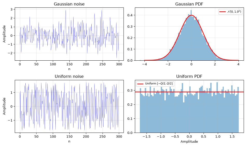
Uniform distribution. Quantization noise is approximately uniformly distributed over \([-Q/2, Q/2]\), where \(Q\) is the quantization step size. A uniform distribution has:
Figure 1: Amplitude distributions of Gaussian (thermal) and uniform (quantization) noise. Left: time-domain samples. Right: histograms with theoretical PDFs overlaid.
Notice the Gaussian noise has occasional large excursions (the “tails” of the bell curve), while the uniform noise is strictly bounded. This difference matters in practice: a Gaussian noise sample can, in theory, exceed any threshold; it’s just increasingly unlikely.
Stationarity and ergodicity
One more concept we’ll need: a random process is stationary if its statistical properties (mean, variance, distribution) do not change over time. Most noise models in DSP assume stationarity: the noise “looks the same” whether you observe it now or later.
A stationary process is ergodic if time averages equal ensemble averages. This is what lets us estimate \(\sigma^2\) from a single long recording rather than needing many independent realisations. In practice, most stationary noise processes we encounter are ergodic, so we freely swap between the two, though this is a working assumption to keep in mind, since it breaks down for non-stationary signals or processes with very long-range correlations.
Exercise: Variance from samples
Generate 1000 samples of Gaussian noise with \(\sigma = 2\) in Python. Estimate the variance from the samples and compare with the true value. How close is the estimate?
Three properties make autocorrelation fundamental:
At zero lag, it equals the signal power: \(R_{xx}[0] = E[x^2] = \sigma^2 + \mu^2\) (for zero-mean signals, \(R_{xx}[0] = \sigma^2\)).
It is symmetric: \(R_{xx}[k] = R_{xx}[-k]\).
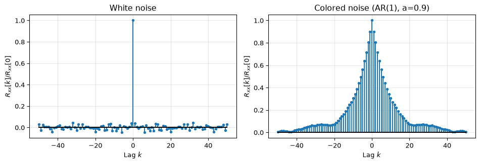
For white noise: \(R_{xx}[k] = \sigma^2\,\delta[k]\): samples are uncorrelated at all nonzero lags.
This last property is what defines white noise: no correlation between any two distinct samples. Colored noise, by contrast, has autocorrelation that decays gradually: nearby samples are correlated.
Figure 2: Autocorrelation of white noise (left) and colored noise (right). White noise is uncorrelated at all nonzero lags; colored noise shows structure.
Autocorrelation connects directly to several concepts we’ll meet later: the power spectral density in Chapter 5 is the Fourier transform of the autocorrelation (the Wiener–Khinchin theorem), and matched filtering is optimal precisely because it exploits the autocorrelation structure of the signal.
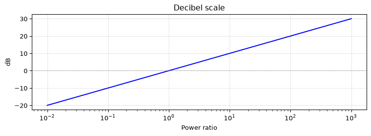
The decibel scale
Signal and noise levels span many orders of magnitude, so we use a logarithmic scale. The decibel (dB) expresses the ratio of two power levels:
For zero-mean discrete signals, power equals the variance, the mean squared value:
\[P = \frac{1}{N} \sum_{n=0}^{N-1} |x[n]|^2\]
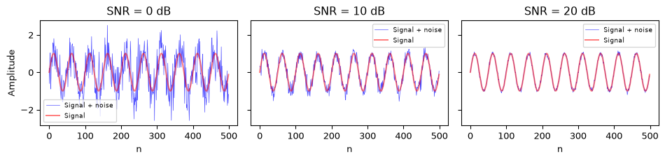
An SNR of 0 dB means the signal and noise have equal power; the signal is barely detectable. At 20 dB, the signal is 100 times stronger than the noise. At 60 dB, the signal is a million times stronger.
Figure 4: The same sinusoid at different SNR levels. At 0 dB the signal is barely visible; at 20 dB it is clean.
Measuring SNR in practice
To compute SNR, you need to separate the signal from the noise. There are several approaches depending on the situation:
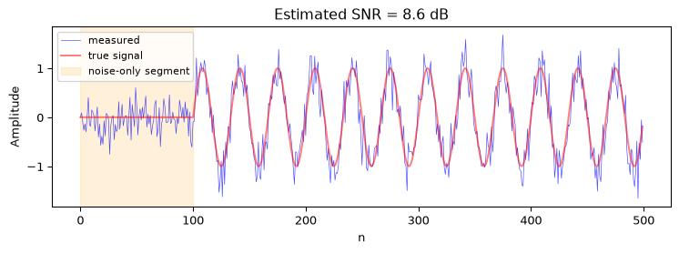
When you have a noise-only segment. If you can identify a portion of the recording that contains only noise (e.g., before the signal starts), estimate \(P_\text{noise}\) from that segment and \(P_\text{signal+noise}\) from the active segment:
When the signal is periodic. Average many periods: the noise averages out while the signal reinforces. The difference between a single period and the average gives the noise estimate.
When you have a known reference. In test scenarios, you can play a known signal, record it, and compute the residual after subtracting the reference.
Figure 5: Measuring SNR using a noise-only segment. The first 100 samples contain only noise; the rest contain signal + noise.
Quantization SNR
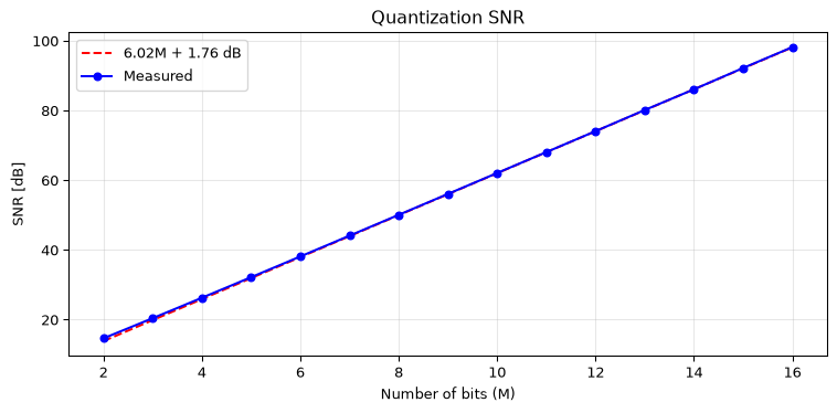
For a full-scale sinusoidal input, the SNR of an ideal \(M\)-bit ADC has a well-known closed-form result:
\[\text{SNR}_\text{dB} = 6.02 \, M + 1.76 \quad \text{[dB]}\]
This is one of the most important numbers in digital audio and data acquisition (Proakis and Manolakis 2007). It tells you that each additional bit of resolution adds approximately 6 dB of SNR.
Bits
SNR (dB)
Dynamic range
8
49.9
Low-quality audio
12
74.0
Instrumentation, industrial
16
98.1
CD-quality audio
24
146.2
Professional audio, measurement
Derivation
For a sinusoid with peak amplitude \(A\) and uniform quantization noise over \([-Q/2, Q/2]\):
Signal power: \(P_\text{signal} = A^2/2\)
Quantization step: \(Q = 2A / (2^M - 1) \approx 2A / 2^M\) for large \(M\)
Figure 6: Quantization SNR: measured vs theoretical. Each bit adds ~6 dB.
Exercise 1
A 12-bit ADC has an input range of 0–3.3 V. What is the quantization step size? What is the theoretical SNR for a full-scale sinusoidal input? Express your answer in dB.
Assuming a full-scale sinusoidal input (centred at 1.65 V with amplitude 1.65 V):
\(\text{SNR} = 6.02 \times 12 + 1.76 = 74.0\) dB.
Improving SNR by averaging
If a measurement is repeatable, you can improve SNR by averaging \(K\) measurements. The key requirement is that the noise in each measurement is independent: knowing one noise realisation tells you nothing about the others. Each measurement contains the same signal \(s[n]\) plus independent noise \(v_k[n]\):
The signal is unchanged, but the noise power reduces by a factor of \(K\):
\[\text{SNR}_\text{averaged} = K \cdot \text{SNR}_\text{single}\]
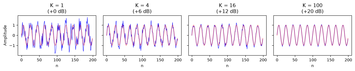
In decibels: averaging \(K\) measurements improves SNR by \(10\log_{10}(K)\) dB. To gain 20 dB, you need 100 averages. This is the \(\sqrt{K}\) law. The noise amplitude decreases as \(1/\sqrt{K}\).
Figure 7: SNR improvement by averaging. 100 averages gives 20 dB improvement, reducing noise by a factor of 10 in amplitude.
Exercise 2
You have a sensor with an SNR of 20 dB. How many averages do you need to achieve 40 dB? What about 60 dB? Is 60 dB realistic in practice?
Solution
40 dB needs a 20 dB improvement → \(K = 10^{20/10} = 100\) averages.
60 dB needs a 40 dB improvement → \(K = 10^{40/10} = 10{,}000\) averages.
Whether 10,000 averages is realistic depends on the measurement time. If each measurement takes 1 ms, you need 10 seconds, feasible for a static signal. But if the signal changes over those 10 seconds, averaging will blur the signal along with the noise.
White noise and colored noise
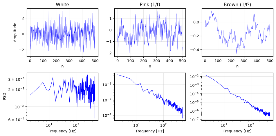
White noise has equal power at all frequencies: its power spectral density (PSD) is flat. This is the simplest noise model and the one assumed in most textbook derivations.
Colored noise has a non-flat PSD. Common types:
Pink noise (1/f): PSD falls as \(1/f\). Common in electronic circuits and natural phenomena (Kasdin 1995).
Brown noise (1/f²): PSD falls as \(1/f^2\). The cumulative sum (discrete integration) of white noise.
Blue noise (f): power rises with frequency. Less common but appears in some digital systems.
The color of noise matters because filters and averaging behave differently depending on the noise spectrum. A low-pass filter that removes half the bandwidth removes half the white noise power (3 dB improvement), but removes much less pink noise power because most pink noise energy is already at low frequencies where the filter passes.
from scipy import signal as sigrng = np.random.default_rng(42)n =4096fs =1000white = rng.standard_normal(n)# Generate pink noise (1/f) by filtering white noise# Approximate 1/f spectrum using Voss-McCartney methodfreqs = np.fft.rfftfreq(n, 1/fs)freqs[0] =1# avoid division by zerowhite_fft = np.fft.rfft(white)pink = np.fft.irfft(white_fft / np.sqrt(freqs), n)pink = pink / np.std(pink)# Brown noise: cumulative sum of white noisebrown = np.cumsum(white)brown = brown / np.std(brown)fig, axes = plt.subplots(2, 3, figsize=(10, 5))names = ['White', 'Pink (1/f)', 'Brown (1/f²)']signals = [white, pink, brown]for i, (name, s) inenumerate(zip(names, signals)): axes[0, i].plot(s[:500], 'b-', linewidth=0.3) axes[0, i].set_title(name) axes[0, i].set_xlabel('n') axes[0, i].grid(True, alpha=0.3)if i ==0: axes[0, i].set_ylabel('Amplitude') f, psd = sig.welch(s, fs, nperseg=512) axes[1, i].loglog(f[1:], psd[1:], 'b-', linewidth=0.8) axes[1, i].set_xlabel('Frequency [Hz]')if i ==0: axes[1, i].set_ylabel('PSD') axes[1, i].grid(True, alpha=0.3)fig.tight_layout()plt.show()
Figure 8: White, pink, and brown noise: time domain (top) and power spectral density (bottom).
For a deeper treatment of colored noise (including how to characterise the spectral exponent and whiten the noise before further processing), see the noise whitening topic.
SNR and filtering
A filter changes both the signal and the noise. Whether SNR improves depends on how much signal and noise overlap in frequency.
If the signal occupies a narrow frequency band and the noise is white (spread across all frequencies), a bandpass filter that passes only the signal’s band rejects most of the noise. The SNR improvement depends on the ratio of signal bandwidth to total bandwidth.
The theoretical limit of this idea is the matched filter: a filter whose impulse response is tailored to the exact shape of the expected signal. It can be shown that the matched filter maximises the output SNR; no other linear filter does better. See the matched filtering topic for the full derivation and applications.
Exercise 3
A signal occupies the band 100–200 Hz. Noise is white across 0–5000 Hz (the Nyquist bandwidth at \(f_s\) = 10 kHz). By how many dB does a perfect bandpass filter (passing 100–200 Hz, rejecting everything else) improve the SNR?
Solution
The noise is white, so noise power is proportional to bandwidth.
Before filtering: noise bandwidth = 5000 Hz. After filtering: noise bandwidth = 100 Hz.
The next chapter introduces the mathematical framework that makes frequency-domain analysis precise: The z-domain.
References
Kasdin, N. Jeremy. 1995. “Discrete Simulation of Colored Noise and Stochastic Processes and 1/f^α Power Law Noise Generation.”Proceedings of the IEEE 83 (5): 802–27. https://doi.org/10.1109/5.381848.
Papoulis, Athanasios, and S. Unnikrishna Pillai. 2002. Probability, Random Variables, and Stochastic Processes. 4th ed. McGraw-Hill.
Proakis, John G., and Dimitris G. Manolakis. 2007. Digital Signal Processing: Principles, Algorithms, and Applications. 4th ed. Pearson.
Source Code
---title: "Noise and SNR"---```{python}#| echo: falseimport numpy as npimport matplotlib.pyplot as plt```Every real measurement contains noise. Whether it comes from thermal agitation in a resistor, rounding errors in an ADC, or electromagnetic interference from a nearby motor, the signal you want is always mixed with something you do not want.Understanding noise is not optional in DSP. Many design decisions (how many bits to use, what sample rate to choose, which filter to apply) come down in large part to one question: *how much noise can we tolerate?*---## What is noise?Noise is any *random* unwanted component added to a signal: you cannot predict the next sample from previous ones. In DSP, the main sources of noise are:- **Thermal noise** (Johnson–Nyquist noise): caused by random motion of charge carriers in any conductor. Present in every electronic component, at every frequency, with a flat power spectrum. This is the physical floor; you cannot eliminate it.- **Quantization noise**: the error introduced when a continuous value is rounded to the nearest digital level. For a well-designed ADC, this behaves approximately like uniform white noise with variance $Q^2/12$, where $Q$ is the step size (see [Chapter 1](01-signals.qmd)).- **Flicker noise** (1/f noise): present in almost all electronic devices, with power spectral density proportional to $1/f^\alpha$. Dominant at low frequencies. See the [noise whitening](../topics/noise-whitening/index.qmd) topic for a deeper treatment.Besides noise, measurements are often corrupted by **interference**: deterministic signals coupling into the measurement path: mains hum (50/60 Hz), switching noise from power supplies, crosstalk from adjacent channels. Interference is not noise, but in practice it can look like it.::: {.callout-note}## Noise vs interferenceNoise is *random*; interference is *deterministic*: in principle, you can model and subtract it. The distinction matters because different techniques apply: filtering and averaging reduce random noise; synchronous detection and notch filters remove interference.:::---## Describing noise: random variables and distributionsNoise is random, so we need the language of probability to describe it. A **random variable** $X$ is a quantity whose value is determined by a random process: the voltage at a sensor output at a given instant, or the quantization error of a single sample.### Mean and varianceThe **expected value** (or mean) $\mu$ of a random variable tells you where the distribution is centred:$$\mu = E[X]$$The **variance** $\sigma^2$ tells you how spread out the values are around the mean:$$\sigma^2 = E\bigl[(X - \mu)^2\bigr] = E[X^2] - \mu^2$$The square root $\sigma$ is the **standard deviation**: it has the same units as $X$, making it easier to interpret. For zero-mean noise ($\mu = 0$), the variance equals the mean squared value: $\sigma^2 = E[X^2]$. This is why **variance and power are the same thing** for zero-mean signals, a connection we'll use throughout this chapter.In practice, we estimate these from $N$ samples:$$\hat{\mu} = \frac{1}{N}\sum_{n=0}^{N-1} x[n], \qquad \hat{\sigma}^2 = \frac{1}{N}\sum_{n=0}^{N-1} (x[n] - \hat{\mu})^2$$### Amplitude distributionsThe **probability density function** (PDF) describes how likely different amplitude values are. Two distributions dominate DSP:**Gaussian (normal) distribution.** Thermal noise follows a Gaussian distribution with mean $\mu$ and variance $\sigma^2$:$$p(x) = \frac{1}{\sigma\sqrt{2\pi}} \exp\!\left(-\frac{(x-\mu)^2}{2\sigma^2}\right)$$The Gaussian is central to DSP because of the **central limit theorem** [@papoulis2002probability]: the sum of many independent random effects tends toward a Gaussian distribution, regardless of the individual distributions. Since thermal noise arises from billions of independent charge carrier collisions, it is very nearly Gaussian.**Uniform distribution.** Quantization noise is approximately uniformly distributed over $[-Q/2, Q/2]$, where $Q$ is the quantization step size. A uniform distribution has:$$\mu = 0, \qquad \sigma^2 = \frac{Q^2}{12}$$```{python}#| label: fig-distributions#| fig-cap: "Amplitude distributions of Gaussian (thermal) and uniform (quantization) noise. Left: time-domain samples. Right: histograms with theoretical PDFs overlaid."rng = np.random.default_rng(42)N =10000sigma =1.0gaussian = rng.normal(0, sigma, N)Q = np.sqrt(12) * sigma # same variance as Gaussian for fair comparisonuniform = rng.uniform(-Q/2, Q/2, N)fig, axes = plt.subplots(2, 2, figsize=(10, 6))# Time-domain samplesfor ax, data, name inzip(axes[:, 0], [gaussian, uniform], ['Gaussian', 'Uniform']): ax.plot(data[:300], 'b-', linewidth=0.3) ax.set_ylabel('Amplitude') ax.set_title(f'{name} noise') ax.set_xlabel('n') ax.grid(True, alpha=0.3)# Histograms with theoretical PDFsx_range = np.linspace(-4*sigma, 4*sigma, 200)axes[0, 1].hist(gaussian, bins=80, density=True, alpha=0.5, color='C0')pdf_gauss = np.exp(-x_range**2/ (2*sigma**2)) / (sigma * np.sqrt(2*np.pi))axes[0, 1].plot(x_range, pdf_gauss, 'r-', linewidth=2, label=f'$\\mathcal{{N}}(0, {sigma}^2)$')axes[0, 1].set_title('Gaussian PDF')axes[0, 1].legend(fontsize=8)axes[0, 1].grid(True, alpha=0.3)axes[1, 1].hist(uniform, bins=80, density=True, alpha=0.5, color='C0')axes[1, 1].axhline(1/Q, color='r', linewidth=2, label=f'Uniform $[-Q/2, Q/2]$')axes[1, 1].set_title('Uniform PDF')axes[1, 1].set_xlabel('Amplitude')axes[1, 1].legend(fontsize=8)axes[1, 1].grid(True, alpha=0.3)fig.tight_layout()plt.show()```Notice the Gaussian noise has occasional large excursions (the "tails" of the bell curve), while the uniform noise is strictly bounded. This difference matters in practice: a Gaussian noise sample can, in theory, exceed any threshold; it's just increasingly unlikely.### Stationarity and ergodicityOne more concept we'll need: a random process is **stationary** if its statistical properties (mean, variance, distribution) do not change over time. Most noise models in DSP assume stationarity: the noise "looks the same" whether you observe it now or later.A stationary process is **ergodic** if time averages equal ensemble averages. This is what lets us estimate $\sigma^2$ from a single long recording rather than needing many independent realisations. In practice, most stationary noise processes we encounter are ergodic, so we freely swap between the two, though this is a working assumption to keep in mind, since it breaks down for non-stationary signals or processes with very long-range correlations.::: {.callout-tip collapse="true" title="Exercise: Variance from samples"}Generate 1000 samples of Gaussian noise with $\sigma = 2$ in Python. Estimate the variance from the samples and compare with the true value. How close is the estimate?::: {.callout-note collapse="true" title="Answer"}```{python}rng = np.random.default_rng(0)x = rng.normal(0, 2, 1000)print(f"True variance: {2**2}")print(f"Estimated variance: {np.var(x):.3f}")print(f"Estimated std dev: {np.std(x):.3f}")```The estimate is close but not exact: with 1000 samples you typically get within a few percent of the true value.::::::### AutocorrelationThe **autocorrelation function** [@papoulis2002probability] measures how similar a signal is to a delayed copy of itself:$$R_{xx}[k] = E\bigl[x[n]\,x[n+k]\bigr]$$where $k$ is the lag (number of samples of delay). For stationary, ergodic signals we estimate it from data:$$\hat{R}_{xx}[k] = \frac{1}{N} \sum_{n=0}^{N-1-|k|} x[n]\,x[n+|k|]$$Three properties make autocorrelation fundamental:- **At zero lag, it equals the signal power**: $R_{xx}[0] = E[x^2] = \sigma^2 + \mu^2$ (for zero-mean signals, $R_{xx}[0] = \sigma^2$).- **It is symmetric**: $R_{xx}[k] = R_{xx}[-k]$.- **For white noise**: $R_{xx}[k] = \sigma^2\,\delta[k]$: samples are uncorrelated at all nonzero lags.This last property is what *defines* white noise: no correlation between any two distinct samples. Colored noise, by contrast, has autocorrelation that decays gradually: nearby samples are correlated.```{python}#| label: fig-autocorrelation#| fig-cap: "Autocorrelation of white noise (left) and colored noise (right). White noise is uncorrelated at all nonzero lags; colored noise shows structure."rng = np.random.default_rng(42)N =2000white = rng.standard_normal(N)# Colored noise: lowpass-filtered white noisefrom scipy.signal import lfiltercolored = lfilter([1], [1, -0.9], white)fig, axes = plt.subplots(1, 2, figsize=(10, 3.5))for ax, data, name inzip(axes, [white, colored], ['White noise', 'Colored noise (AR(1), a=0.9)']):# Compute normalized autocorrelation lags = np.arange(-50, 51) r = np.correlate(data - np.mean(data), data - np.mean(data), mode='full') r = r / r[N -1] # normalize so R[0] = 1 mid = N -1 ax.stem(lags, r[mid -50:mid +51], linefmt='C0-', markerfmt='C0.', basefmt='k-') ax.set_xlabel('Lag $k$') ax.set_ylabel('$R_{xx}[k] / R_{xx}[0]$') ax.set_title(name) ax.grid(True, alpha=0.3)fig.tight_layout()plt.show()```Autocorrelation connects directly to several concepts we'll meet later: the power spectral density in [Chapter 5](05-frequency-domain.qmd) is the Fourier transform of the autocorrelation (the Wiener–Khinchin theorem), and [matched filtering](../topics/matched-filtering/index.qmd) is optimal precisely because it exploits the autocorrelation structure of the signal.---## The decibel scaleSignal and noise levels span many orders of magnitude, so we use a logarithmic scale. The **decibel** (dB) expresses the ratio of two power levels:$$L = 10 \log_{10} \frac{P}{P_\text{ref}} \quad \text{[dB]}$$Since power is proportional to the square of amplitude, the same ratio in terms of amplitudes (voltages, pressures) is:$$L = 20 \log_{10} \frac{A}{A_\text{ref}} \quad \text{[dB]}$$Some useful reference points:| Ratio (power) | dB ||---|---|| 1 | 0 dB || 2 | 3 dB || 10 | 10 dB || 100 | 20 dB || 1000 | 30 dB || 1/2 | −3 dB |Doubling the power adds 3 dB. Doubling the amplitude adds 6 dB. These two facts cover most mental arithmetic in DSP.```{python}#| label: fig-db-scale#| fig-cap: "The decibel scale: power ratio vs dB. Note the logarithmic compression: a factor-1000 ratio is only 30 dB."ratios = np.logspace(-2, 3, 200)db =10* np.log10(ratios)fig, ax = plt.subplots(figsize=(8, 3))ax.semilogx(ratios, db, 'b-', linewidth=1.5)ax.axhline(0, color='gray', linestyle='--', linewidth=0.5)ax.set_xlabel('Power ratio')ax.set_ylabel('dB')ax.set_title('Decibel scale')ax.grid(True, alpha=0.3)fig.tight_layout()plt.show()```---## Signal-to-noise ratioThe **signal-to-noise ratio** (SNR) quantifies how much stronger the desired signal is compared to the noise:$$\text{SNR} = \frac{P_\text{signal}}{P_\text{noise}}$$In decibels:$$\text{SNR}_\text{dB} = 10 \log_{10} \frac{P_\text{signal}}{P_\text{noise}}$$For zero-mean discrete signals, power equals the variance, the mean squared value:$$P = \frac{1}{N} \sum_{n=0}^{N-1} |x[n]|^2$$An SNR of 0 dB means the signal and noise have equal power; the signal is barely detectable. At 20 dB, the signal is 100 times stronger than the noise. At 60 dB, the signal is a million times stronger.```{python}#| label: fig-snr-examples#| fig-cap: "The same sinusoid at different SNR levels. At 0 dB the signal is barely visible; at 20 dB it is clean."rng = np.random.default_rng(42)n =500t = np.arange(n)signal = np.sin(2* np.pi *0.02* t)fig, axes = plt.subplots(1, 3, figsize=(10, 2.5), sharey=True)for ax, snr_db inzip(axes, [0, 10, 20]): noise_power = np.mean(signal **2) *10** (-snr_db /10) noise = rng.normal(0, np.sqrt(noise_power), n) ax.plot(t, signal + noise, 'b-', linewidth=0.5, alpha=0.7, label='Signal + noise') ax.plot(t, signal, 'r-', linewidth=1.5, alpha=0.5, label='Signal') ax.set_title(f'SNR = {snr_db} dB') ax.set_xlabel('n') ax.legend(fontsize=7)axes[0].set_ylabel('Amplitude')fig.tight_layout()plt.show()```---## Measuring SNR in practiceTo compute SNR, you need to separate the signal from the noise. There are several approaches depending on the situation:**When you have a noise-only segment.** If you can identify a portion of the recording that contains only noise (e.g., before the signal starts), estimate $P_\text{noise}$ from that segment and $P_\text{signal+noise}$ from the active segment:$$P_\text{signal} \approx P_\text{signal+noise} - P_\text{noise}$$**When the signal is periodic.** Average many periods: the noise averages out while the signal reinforces. The difference between a single period and the average gives the noise estimate.**When you have a known reference.** In test scenarios, you can play a known signal, record it, and compute the residual after subtracting the reference.```{python}#| label: fig-snr-measurement#| fig-cap: "Measuring SNR using a noise-only segment. The first 100 samples contain only noise; the rest contain signal + noise."rng = np.random.default_rng(7)n_noise =100n_total =500# Build a signal that starts after n_noise samplessignal = np.zeros(n_total)signal[n_noise:] = np.sin(2* np.pi *0.03* np.arange(n_total - n_noise))noise =0.3* rng.standard_normal(n_total)measured = signal + noise# Estimate SNRp_noise = np.mean(measured[:n_noise] **2)p_total = np.mean(measured[n_noise:] **2)p_signal = p_total - p_noisesnr_est =10* np.log10(p_signal / p_noise)fig, ax = plt.subplots(figsize=(8, 3))ax.plot(measured, 'b-', linewidth=0.5, alpha=0.7, label='measured')ax.plot(signal, 'r-', linewidth=1.5, alpha=0.5, label='true signal')ax.axvspan(0, n_noise, alpha=0.15, color='orange', label='noise-only segment')ax.set_xlabel('n')ax.set_ylabel('Amplitude')ax.set_title(f'Estimated SNR = {snr_est:.1f} dB')ax.legend(fontsize=8)fig.tight_layout()plt.show()```---## Quantization SNRFor a full-scale sinusoidal input, the SNR of an ideal $M$-bit ADC has a well-known closed-form result:$$\text{SNR}_\text{dB} = 6.02 \, M + 1.76 \quad \text{[dB]}$$This is one of the most important numbers in digital audio and data acquisition [@proakis2007digital]. It tells you that **each additional bit of resolution adds approximately 6 dB of SNR**.| Bits | SNR (dB) | Dynamic range ||---|---|---|| 8 | 49.9 | Low-quality audio || 12 | 74.0 | Instrumentation, industrial || 16 | 98.1 | CD-quality audio || 24 | 146.2 | Professional audio, measurement |::: {.callout-tip collapse="true"}## DerivationFor a sinusoid with peak amplitude $A$ and uniform quantization noise over $[-Q/2, Q/2]$:- Signal power: $P_\text{signal} = A^2/2$- Quantization step: $Q = 2A / (2^M - 1) \approx 2A / 2^M$ for large $M$- Noise power: $P_\text{noise} = Q^2 / 12$- Substituting $Q \approx 2A/2^M$: SNR $= 6A^2/Q^2 = 6A^2 / (4A^2/2^{2M}) = \tfrac{3}{2} \cdot 2^{2M}$In dB: $\text{SNR} = 10\log_{10}(3/2) + 20M\log_{10}(2) = 1.76 + 6.02M$:::```{python}#| label: fig-quantization-snr#| fig-cap: "Quantization SNR: measured vs theoretical. Each bit adds ~6 dB."def quantize(x, bits): scale =2** (bits -1)return np.clip(np.round(x * scale) / scale, -1.0, 1.0)t = np.linspace(0, 10, 10000)signal = np.sin(2* np.pi * t)bits_range = np.arange(2, 17)snr_measured = []snr_theory =6.02* bits_range +1.76for b in bits_range: q = quantize(signal, b) noise = signal - q p_s = np.mean(signal **2) p_n = np.mean(noise **2) snr_measured.append(10* np.log10(p_s / p_n) if p_n >0else100)fig, ax = plt.subplots(figsize=(8, 4))ax.plot(bits_range, snr_theory, 'r--', linewidth=1.5, label='6.02M + 1.76 dB')ax.plot(bits_range, snr_measured, 'bo-', markersize=5, label='Measured')ax.set_xlabel('Number of bits (M)')ax.set_ylabel('SNR [dB]')ax.set_title('Quantization SNR')ax.legend()ax.grid(True, alpha=0.3)fig.tight_layout()plt.show()```::: {.callout-note}## Exercise 1A 12-bit ADC has an input range of 0–3.3 V. What is the quantization step size? What is the theoretical SNR for a full-scale sinusoidal input? Express your answer in dB.::: {.callout-tip collapse="true"}## Solution$Q = 3.3 / (2^{12} - 1) = 3.3/4095 \approx 0.806$ mV.Assuming a full-scale sinusoidal input (centred at 1.65 V with amplitude 1.65 V):$\text{SNR} = 6.02 \times 12 + 1.76 = 74.0$ dB.::::::---## Improving SNR by averagingIf a measurement is repeatable, you can improve SNR by averaging $K$ measurements. The key requirement is that the noise in each measurement is **independent**: knowing one noise realisation tells you nothing about the others. Each measurement contains the same signal $s[n]$ plus independent noise $v_k[n]$:$$\bar{x}[n] = \frac{1}{K} \sum_{k=1}^{K} (s[n] + v_k[n]) = s[n] + \frac{1}{K} \sum_{k=1}^{K} v_k[n]$$The signal is unchanged, but the noise power reduces by a factor of $K$:$$\text{SNR}_\text{averaged} = K \cdot \text{SNR}_\text{single}$$In decibels: averaging $K$ measurements improves SNR by $10\log_{10}(K)$ dB. To gain 20 dB, you need 100 averages. This is the **$\sqrt{K}$ law**. The noise amplitude decreases as $1/\sqrt{K}$.```{python}#| label: fig-averaging#| fig-cap: "SNR improvement by averaging. 100 averages gives 20 dB improvement, reducing noise by a factor of 10 in amplitude."rng = np.random.default_rng(42)n =200signal = np.sin(2* np.pi *0.05* np.arange(n))K_values = [1, 4, 16, 100]fig, axes = plt.subplots(1, 4, figsize=(12, 2.5), sharey=True)for ax, K inzip(axes, K_values): measurements = signal[None, :] +0.5* rng.standard_normal((K, n)) averaged = measurements.mean(axis=0) ax.plot(averaged, 'b-', linewidth=0.7) ax.plot(signal, 'r-', linewidth=1.5, alpha=0.4) improvement =10* np.log10(K) ax.set_title(f'K = {K}\n(+{improvement:.0f} dB)') ax.set_xlabel('n')axes[0].set_ylabel('Amplitude')fig.tight_layout()plt.show()```::: {.callout-note}## Exercise 2You have a sensor with an SNR of 20 dB. How many averages do you need to achieve 40 dB? What about 60 dB? Is 60 dB realistic in practice?::: {.callout-tip collapse="true"}## Solution40 dB needs a 20 dB improvement → $K = 10^{20/10} = 100$ averages.60 dB needs a 40 dB improvement → $K = 10^{40/10} = 10{,}000$ averages.Whether 10,000 averages is realistic depends on the measurement time. If each measurement takes 1 ms, you need 10 seconds, feasible for a static signal. But if the signal changes over those 10 seconds, averaging will blur the signal along with the noise.::::::---## White noise and colored noise**White noise** has equal power at all frequencies: its power spectral density (PSD) is flat. This is the simplest noise model and the one assumed in most textbook derivations.**Colored noise** has a non-flat PSD. Common types:- **Pink noise** (1/f): PSD falls as $1/f$. Common in electronic circuits and natural phenomena [@kasdin1995discrete].- **Brown noise** (1/f²): PSD falls as $1/f^2$. The cumulative sum (discrete integration) of white noise.- **Blue noise** (f): power rises with frequency. Less common but appears in some digital systems.The color of noise matters because filters and averaging behave differently depending on the noise spectrum. A low-pass filter that removes half the bandwidth removes half the *white* noise power (3 dB improvement), but removes much less *pink* noise power because most pink noise energy is already at low frequencies where the filter passes.```{python}#| label: fig-noise-colors#| fig-cap: "White, pink, and brown noise: time domain (top) and power spectral density (bottom)."from scipy import signal as sigrng = np.random.default_rng(42)n =4096fs =1000white = rng.standard_normal(n)# Generate pink noise (1/f) by filtering white noise# Approximate 1/f spectrum using Voss-McCartney methodfreqs = np.fft.rfftfreq(n, 1/fs)freqs[0] =1# avoid division by zerowhite_fft = np.fft.rfft(white)pink = np.fft.irfft(white_fft / np.sqrt(freqs), n)pink = pink / np.std(pink)# Brown noise: cumulative sum of white noisebrown = np.cumsum(white)brown = brown / np.std(brown)fig, axes = plt.subplots(2, 3, figsize=(10, 5))names = ['White', 'Pink (1/f)', 'Brown (1/f²)']signals = [white, pink, brown]for i, (name, s) inenumerate(zip(names, signals)): axes[0, i].plot(s[:500], 'b-', linewidth=0.3) axes[0, i].set_title(name) axes[0, i].set_xlabel('n') axes[0, i].grid(True, alpha=0.3)if i ==0: axes[0, i].set_ylabel('Amplitude') f, psd = sig.welch(s, fs, nperseg=512) axes[1, i].loglog(f[1:], psd[1:], 'b-', linewidth=0.8) axes[1, i].set_xlabel('Frequency [Hz]')if i ==0: axes[1, i].set_ylabel('PSD') axes[1, i].grid(True, alpha=0.3)fig.tight_layout()plt.show()```For a deeper treatment of colored noise (including how to characterise the spectral exponent and whiten the noise before further processing), see the [noise whitening topic](../topics/noise-whitening/index.qmd).---## SNR and filteringA filter changes both the signal and the noise. Whether SNR improves depends on how much signal and noise overlap in frequency.If the signal occupies a narrow frequency band and the noise is white (spread across all frequencies), a bandpass filter that passes only the signal's band rejects most of the noise. The SNR improvement depends on the ratio of signal bandwidth to total bandwidth.The theoretical limit of this idea is the **matched filter**: a filter whose impulse response is tailored to the exact shape of the expected signal. It can be shown that the matched filter maximises the output SNR; no other linear filter does better. See the [matched filtering topic](../topics/matched-filtering/index.qmd) for the full derivation and applications.::: {.callout-note}## Exercise 3A signal occupies the band 100–200 Hz. Noise is white across 0–5000 Hz (the Nyquist bandwidth at $f_s$ = 10 kHz). By how many dB does a perfect bandpass filter (passing 100–200 Hz, rejecting everything else) improve the SNR?::: {.callout-tip collapse="true"}## SolutionThe noise is white, so noise power is proportional to bandwidth.Before filtering: noise bandwidth = 5000 Hz.After filtering: noise bandwidth = 100 Hz.Improvement = $10\log_{10}(5000/100) = 10\log_{10}(50) \approx 17$ dB.::::::---## Summary| Concept | Key result ||---|---|| SNR definition | $\text{SNR} = P_\text{signal} / P_\text{noise}$ || Decibels | $10\log_{10}(\text{power ratio})$, or $20\log_{10}(\text{amplitude ratio})$ || Quantization SNR | $6.02M + 1.76$ dB for $M$-bit ADC || Averaging | $K$ averages → $+10\log_{10}(K)$ dB || Filtering | Improvement depends on signal vs noise bandwidth || Optimal filter | Matched filter maximises output SNR |Want more practice? See the [Exercise set for Chapter 3](../exercises/03-noise-snr.qmd) for additional problems at varying difficulty levels.::: {.callout-note title="Further reading"}- Papoulis & Pillai, *Probability, Random Variables, and Stochastic Processes* (2002), Ch. 9: Random processes, autocorrelation- Proakis & Manolakis, *Digital Signal Processing* (2007), Ch. 12.2: Quantization noise analysis:::::: {.callout-note title="Going deeper"}Several [Topics](../topics/index.qmd) pages build directly on this chapter:- [Noise whitening](../topics/noise-whitening/index.qmd): characterising colored noise spectra and whitening before further processing- [Matched filtering](../topics/matched-filtering/index.qmd): the SNR-optimal filter for detecting known signals in noise- [Outlier detection](../topics/outlier-detection/index.qmd): robust methods for identifying anomalous samples (three-sigma, Tukey, MAD):::The next chapter introduces the mathematical framework that makes frequency-domain analysis precise: [The z-domain](04-z-domain.qmd).## References::: {#refs}:::