A Tone Tracker on Hardware

Turning the Cramér-Rao bound into an instrument specification, on STM32F4 and ESP32-S3

A microcontroller that measures the frequency of a tone to a few parts per million is an instrument, and it costs a few euros. Vibration monitors, guitar tuners, resonant sensor front ends, motor speed pickups, and LVDT readouts are all this same device with different packaging.

What makes this page different from the other embedded companions is that the theory on the main page does something unusual for DSP theory: it sizes the hardware before you build it. The Cramér-Rao bound depends only on the SNR and the record length, not on any algorithm, so you can answer “how long must I integrate to hit my accuracy spec?” while the board is still a schematic. That is the whole of the first section, and it is the most useful thing here.

Both default platforms per ADR-005: NUCLEO-F446RE (Cortex-M4F, CMSIS-DSP) and ESP32-S3 (Xtensa LX7, ESP-DSP), single-precision float first.

Sizing the instrument before you build it

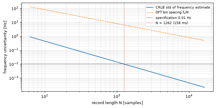
Start from the specification rather than the algorithm. Suppose you need to measure a tone near 1 kHz to a standard deviation of 0.01 Hz, your front end delivers about 20 dB SNR, and you sample at 8 kHz. Rearranging the frequency bound

\[\operatorname{var}(\hat{f_0}) \ge \frac{12 f_s^2}{(2\pi)^2\, \eta\, N(N^2-1)}\]

for $N$ answers the question directly, and the answer is a hard floor: no cleverness in your firmware will beat it.

fs, snr_db, target_hz = 8000.0, 20.0, 0.01
eta = 10 ** (snr_db / 10)
sigma = 1.0 / np.sqrt(2 * eta)                 # unit amplitude, so A^2/(2 sigma^2) = eta

Ns = np.unique(np.logspace(np.log10(64), np.log10(16384), 120).astype(int))
std_hz = np.array([np.sqrt(crlb_sinusoid(1.0, sigma, int(N), fs=fs)['frequency'])
                   for N in Ns])

# Smallest N meeting the spec, found from the curve itself.
ok = np.nonzero(std_hz <= target_hz)[0]
N_required = int(Ns[ok[0]])

fig, ax = plt.subplots(figsize=(7.5, 3.8))
ax.loglog(Ns, std_hz, 'C0', lw=1.5, label='CRLB std of frequency estimate')
ax.loglog(Ns, fs / Ns, 'C1--', lw=1.1, label=r'DFT bin spacing $f_s/N$')
ax.axhline(target_hz, color='k', ls=':', lw=1.2, label=f'specification {target_hz} Hz')
ax.axvline(N_required, color='C3', ls=':', lw=1.2,
           label=f'N = {N_required} ({N_required/fs*1e3:.0f} ms)')
ax.set_xlabel('record length N [samples]'); ax.set_ylabel('frequency uncertainty [Hz]')
ax.grid(True, which='both', alpha=0.3); ax.legend(fontsize=8)
fig.tight_layout(); plt.show()

print(f"spec {target_hz} Hz at {snr_db:.0f} dB SNR, fs = {fs:.0f} Hz")
print(f"  -> N = {N_required} samples = {N_required/fs*1e3:.1f} ms of integration")
for N in (512, 1024, 2048, 4096):
    s = np.sqrt(crlb_sinusoid(1.0, sigma, N, fs=fs)['frequency'])
    print(f"  N = {N:5d} ({N/fs*1e3:6.1f} ms): CRLB std {s:7.4f} Hz, "
          f"bin spacing {fs/N:6.2f} Hz, ratio {(fs/N)/s:5.0f}x")

assert 1200 < N_required < 1300, f"expected ~1260 samples, got {N_required}"
# The caption's "three orders of magnitude" claim, at the chosen size.
ratio = (fs / N_required) / np.sqrt(crlb_sinusoid(1.0, sigma, N_required, fs=fs)['frequency'])
assert 500 < ratio < 1500, f"bin/std ratio {ratio:.0f} outside the quoted range"
# Doubling N must buy the 2^1.5 the 1/N^3 law promises.
s1 = np.sqrt(crlb_sinusoid(1.0, sigma, 1024, fs=fs)['frequency'])
s2 = np.sqrt(crlb_sinusoid(1.0, sigma, 2048, fs=fs)['frequency'])
assert abs(s1 / s2 - 2**1.5) < 0.05, "doubling the record should buy 2.83x"

Figure 1: Sizing the record from the accuracy specification. The curve is the Cramér-Rao standard deviation at 20 dB SNR and fs = 8 kHz; the specification of 0.01 Hz is first met at about 1260 samples, roughly 160 ms of integration. The bin spacing fs/N is drawn for scale: the interpolated estimate is finer than the raw DFT grid by roughly three orders of magnitude, which is why frequency estimation is not the same problem as frequency resolution.

spec 0.01 Hz at 20 dB SNR, fs = 8000 Hz
  -> N = 1262 samples = 157.8 ms of integration
  N =   512 (  64.0 ms): CRLB std  0.0381 Hz, bin spacing  15.62 Hz, ratio   410x
  N =  1024 ( 128.0 ms): CRLB std  0.0135 Hz, bin spacing   7.81 Hz, ratio   580x
  N =  2048 ( 256.0 ms): CRLB std  0.0048 Hz, bin spacing   3.91 Hz, ratio   821x
  N =  4096 ( 512.0 ms): CRLB std  0.0017 Hz, bin spacing   1.95 Hz, ratio  1161x

Three design consequences fall out, and all three are firmware decisions:

Integration time is the currency, and it is cheap. Around 160 ms buys 0.01 Hz. If the spec tightened to 0.001 Hz you would need not ten times but $10^{2/3} \approx 4.6$ times the record, about 730 ms. The $1/N^3$ law is unusually generous, and this is the rare case where the honest engineering answer is “just integrate longer”.

Your bin spacing is not your accuracy. At that record length the DFT bins are about 6.3 Hz apart while the achievable uncertainty is 0.01 Hz, a factor of roughly 600. Interpolation is not a refinement here, it is the entire measurement. Firmware that reports the peak bin index is throwing away nearly all of the available information.

The SNR term is linear, so the analogue front end and the integration time trade directly. 10 dB more SNR is worth a factor of 10 in variance, the same as $10^{1/3} \approx 2.15$ times the record length. A better op-amp and a longer integration are interchangeable, and you should price both.

Two architectures, chosen by what you already know

If the frequency is known (a lock-in front end, a driven resonator, a mains monitor) you need only amplitude and phase, and the Goertzel algorithm computes exactly that single bin with two state variables and no buffer at all. Per sample per bin the inner loop is one multiply and two adds.

If the frequency is unknown, you need a spectrum: buffer $N$ samples, transform, find the peak, interpolate. This costs RAM and an FFT, and it is what most of this page is about.

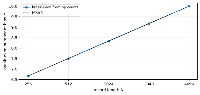
The crossover is worth knowing because it is not where intuition puts it. A real FFT of length $N$ costs roughly $\tfrac{5}{2} N \log_2 N$ flops; $M$ Goertzel bins over the same record cost $3MN$. Setting them equal, Goertzel wins while

\[M \lesssim \tfrac{5}{6} \log_2 N\]

which at $N = 1024$ is about eight bins. Below eight frequencies of interest, skip the FFT; above it, the FFT is already cheaper, and it gives you the whole spectrum for the same price. That figure assumes a real-input FFT, as on the CMSIS path below; the ESP-DSP section revisits it, because running a general complex FFT on a zero-padded real record doubles the FFT side of the comparison.

Ns_x = np.array([256, 512, 1024, 2048, 4096])
fft_flops = 2.5 * Ns_x * np.log2(Ns_x)
breakeven = fft_flops / (3 * Ns_x)

fig, ax = plt.subplots(figsize=(7, 3.4))
ax.semilogx(Ns_x, breakeven, 'o-C0', ms=5, base=2, label='break-even from op counts')
ax.semilogx(Ns_x, (5 / 6) * np.log2(Ns_x), 'k--', lw=1,
            base=2, label=r'$\frac{5}{6}\log_2 N$')
ax.set_xlabel('record length N'); ax.set_ylabel('break-even number of bins M')
ax.set_xticks(Ns_x); ax.set_xticklabels(Ns_x)
ax.grid(True, alpha=0.3); ax.legend(fontsize=8)
fig.tight_layout(); plt.show()

for N, f_, b in zip(Ns_x, fft_flops, breakeven):
    print(f"N = {N:5d}: real FFT ~{f_:8.0f} flops, Goertzel breaks even at "
          f"M = {b:.1f} bins")

# The (5/6) log2 N closed form must reproduce the ratio of the two op counts.
assert np.allclose(breakeven, (5 / 6) * np.log2(Ns_x), rtol=1e-12)
assert 8.0 < breakeven[Ns_x == 1024][0] < 8.5, "expected ~8.3 bins at N=1024"

Figure 2: Where Goertzel stops being the cheap option. Arithmetic-operation counts derived from the inner loops: 3 flops per sample per bin for Goertzel against roughly (5/2)·N·log2(N) for a real FFT of the whole record. The break-even is near (5/6)·log2(N) bins, about eight at N = 1024, and it grows only logarithmically with record length.

N =   256: real FFT ~    5120 flops, Goertzel breaks even at M = 6.7 bins
N =   512: real FFT ~   11520 flops, Goertzel breaks even at M = 7.5 bins
N =  1024: real FFT ~   25600 flops, Goertzel breaks even at M = 8.3 bins
N =  2048: real FFT ~   56320 flops, Goertzel breaks even at M = 9.2 bins
N =  4096: real FFT ~  122880 flops, Goertzel breaks even at M = 10.0 bins

Operation counts are not cycle counts

The numbers above are flops derived from the algorithms’ inner loops, which is what you can reason about on paper. They are not cycle counts. A CMSIS-DSP FFT on an M4F uses SIMD and hand-tuned assembly and will beat a naive flop-ratio prediction; a Goertzel loop is limited by load/store and pipeline behaviour rather than by its single multiply. Use the ratio above to choose an architecture, then measure the real thing on the real part with the cycle counter (DWT->CYCCNT on Cortex-M, esp_cpu_get_cycle_count() on the ESP32-S3) before committing to a sample rate.

The tracker: portable C

The core is deliberately platform-neutral: a windowed real FFT fills a magnitude array, then three bins around the peak produce a fractional bin offset. Only the FFT call differs between the two platforms.

#include <math.h>
#include <stdint.h>

#define NFFT       1024                  // record length, power of two
#define FS_HZ      8000.0f

// Jacobsen's three-bin estimator, for a RECTANGULAR window. See the main
// page: pairing the interpolator with the window matters more than the
// choice of interpolator. With a Hann or Blackman window, use the
// log-parabola below instead; using the wrong one leaves a bias that
// averaging never removes.
static float interp_jacobsen(const float *re, const float *im, int k)
{
    float num_r = re[k - 1] - re[k + 1];
    float num_i = im[k - 1] - im[k + 1];
    float den_r = 2.0f * re[k] - re[k - 1] - re[k + 1];
    float den_i = 2.0f * im[k] - im[k - 1] - im[k + 1];

    float d2 = den_r * den_r + den_i * den_i;
    if (d2 <= 0.0f) return 0.0f;         // flat peak: no information
    return (num_r * den_r + num_i * den_i) / d2;   // Re{num/den}
}

// Log-parabolic interpolation, for a TAPERED window (Hann, Blackman).
static float interp_parabolic(const float *mag, int k)
{
    // Guard the logs: a zeroed bin would otherwise produce -inf.
    const float tiny = 1e-20f;
    float a = logf(mag[k - 1] + tiny);
    float b = logf(mag[k]     + tiny);
    float c = logf(mag[k + 1] + tiny);
    float den = a - 2.0f * b + c;
    if (den == 0.0f) return 0.0f;
    return 0.5f * (a - c) / den;
}

// Peak bin of the one-sided magnitude spectrum, excluding DC and Nyquist:
// neither can host a resolvable tone, and the interpolators need a
// neighbour on each side.
static int peak_bin(const float *mag, int n_bins)
{
    int k = 1;
    for (int i = 2; i < n_bins - 1; i++)
        if (mag[i] > mag[k]) k = i;
    return k;
}

The estimate is then (k + delta) * FS_HZ / NFFT. Note what is not here: no square root is needed to find the peak (compare squared magnitudes), and the interpolation is a handful of flops on three bins regardless of NFFT.

On the STM32F4 (CMSIS-DSP)

arm_rfft_fast_f32 returns the packed one-sided spectrum, with the purely-real DC and Nyquist bins folded into spec[0] and spec[1] and the remaining bins interleaved as real/imaginary pairs. This packing is the single most common source of wrong answers on this API, and it matters more here than usual: Jacobsen’s estimator needs the complex bins, not magnitudes, so the de-interleaving has to be right.

#include "arm_math.h"

static arm_rfft_fast_instance_f32 fft;
static float spec[NFFT];                 // packed output, NFFT floats
static float re[NFFT/2 + 1];             // de-interleaved
static float im[NFFT/2 + 1];
static float mag2[NFFT/2 + 1];           // squared magnitude

void tracker_init(void)
{
    arm_rfft_fast_init_f32(&fft, NFFT);  // once at startup
}

// frame[] holds NFFT real samples, already windowed by the caller.
float tracker_estimate_hz(float *frame)
{
    arm_rfft_fast_f32(&fft, frame, spec, 0);        // 0 = forward

    // Unpack: spec[0] = DC (real), spec[1] = Nyquist (real), then
    // interleaved (re, im) for bins 1 .. NFFT/2 - 1.
    re[0] = spec[0];        im[0] = 0.0f;
    re[NFFT/2] = spec[1];   im[NFFT/2] = 0.0f;
    for (int k = 1; k < NFFT/2; k++) {
        re[k] = spec[2*k];
        im[k] = spec[2*k + 1];
    }
    for (int k = 0; k <= NFFT/2; k++)
        mag2[k] = re[k]*re[k] + im[k]*im[k];        // no sqrt needed

    int k = peak_bin(mag2, NFFT/2 + 1);
    float delta = interp_jacobsen(re, im, k);       // rectangular window
    return (k + delta) * FS_HZ / (float)NFFT;
}

Memory: spec is NFFT floats, re/im/mag2 add another 3(NFFT/2+1), and the caller’s frame is a further NFFT. At NFFT = 1024 that is $1024 + 3 \times 513 + 1024 = 3587$ floats, about 14 kB, comfortable in the F446RE’s 128 kB but worth watching if you scale NFFT up for the accuracy the previous section priced. Dropping mag2 and comparing re*re + im*im inline inside peak_bin saves 2 kB at NFFT = 1024.

On the ESP32-S3 (ESP-DSP)

ESP-DSP’s radix-2 FFT is a complex transform (the fc32 suffix is float-complex, not float-real), so the real frame is packed into the real slots with zeroed imaginary slots, transformed in place, and bit-reversed to unscramble. The complex bins then come straight out of the interleaved array, which suits Jacobsen’s estimator well.

#include "esp_dsp.h"

static float z[2 * NFFT];                // interleaved (re, im)
static float re[NFFT/2 + 1];
static float im[NFFT/2 + 1];
static float mag2[NFFT/2 + 1];

void tracker_init(void)
{
    dsps_fft2r_init_fc32(NULL, NFFT);    // once at startup: twiddle tables
}

float tracker_estimate_hz(float *frame)
{
    for (int n = 0; n < NFFT; n++) {     // real into (re, im) slots
        z[2*n]     = frame[n];
        z[2*n + 1] = 0.0f;
    }
    dsps_fft2r_fc32(z, NFFT);            // in-place radix-2
    dsps_bit_rev_fc32(z, NFFT);          // unscramble

    for (int k = 0; k <= NFFT/2; k++) {  // one-sided half is all we need
        re[k] = z[2*k];
        im[k] = z[2*k + 1];
        mag2[k] = re[k]*re[k] + im[k]*im[k];
    }

    int k = peak_bin(mag2, NFFT/2 + 1);
    float delta = interp_jacobsen(re, im, k);
    return (k + delta) * FS_HZ / (float)NFFT;
}

The complex packing costs both memory and arithmetic, and the arithmetic is the part that surprises people. z alone is $2 \times 1024$ floats, so the ESP-DSP path uses about 8 kB where the CMSIS real FFT uses 4 kB for its output. Less obviously, dsps_fft2r_fc32 is a general complex FFT: it has no way to know the imaginary half you handed it is all zeros, so it runs the full complex butterfly count, roughly $5N\log_2 N$ flops, against about $2.5N\log_2 N$ for a real-input FFT that exploits the symmetry. At NFFT = 1024 that is around 51 000 flops versus 25 600, plus a full-length dsps_bit_rev_fc32 pass the CMSIS packed path does not need.

So the crossover figure from the previous section, about eight bins at $N = 1024$, is the CMSIS/real-FFT number. On the ESP-DSP path as written the FFT side of that comparison doubles, and Goertzel stays competitive until roughly

\[M \lesssim \tfrac{5}{3} \log_2 N \qquad (\approx 17 \text{ bins at } N = 1024)\]

If you need the real-FFT cost back, ESP-DSP’s documented recipe packs $N$ real samples into $N/2$ complex ones, transforms at half length, and splits the result with dsps_cplx2reC_fc32. That is genuinely cheaper, but it changes the output bin layout that the Jacobsen unpack above depends on, so treat it as a deliberate optimisation to be re-verified against the library’s own example rather than a drop-in substitution.

Getting the record you need

Two practical points connect the theory to the ADC.

Window only if you must. The rectangular window is optimal for white noise, and the coherent case on the main page is exactly optimal when the record spans whole cycles. Window when a second tone or a strong nearby interferer would otherwise leak into your peak, and then switch the interpolator to the parabolic form to match. Windowing “just to be safe” costs both noise performance and, if you forget to change interpolators, a systematic bias.

Watch the SNR you actually have, not the one on the datasheet. The bound is driven by $\eta$ at the ADC, after the front end, after any anti-alias filtering, and including quantisation noise. If you are within a few dB of the ADC’s own noise floor, that floor is your $\eta$ and no integration time fixes a front end that is throwing information away before the converter sees it.

Below threshold, do not report a number. The threshold effect means a low-SNR estimate is not a noisy answer, it is often an entirely wrong one. An instrument should know this about itself: compare the peak against the median of the spectrum, and refuse to report a frequency when the ratio is too small. A tuner that says “no signal” is more useful than one that confidently displays a number drawn from a coin flip.

// A cheap, robust guard: peak-to-median ratio of the power spectrum.
// The median tracks the noise floor and ignores the tone itself, so it
// stays honest where a mean would be dragged up by the peak.
static int peak_is_credible(const float *mag2, int n_bins, int k, float min_ratio)
{
    // Partial selection is enough; a full sort is wasted work here.
    float floor_est = median_of(mag2, n_bins);   // e.g. quickselect
    return mag2[k] > min_ratio * floor_est;
}

When there is no FPU

On a Cortex-M0+ or an AVR, the float FFT above is out of reach and you move to arm_rfft_q15 or an integer FFT of your own. The architecture survives unchanged; two things need care. Every FFT stage needs scaling to stay inside 16 bits, so the finite word-length discipline applies throughout, and the interpolation must be done in a wider type: the differences 2*re[k] - re[k-1] - re[k+1] are small quantities between large ones, exactly the cancellation that eats fixed-point precision. Compute the interpolation in Q31 or in software float even when the FFT is Q15, or you will spend the accuracy the bound promised you.

If the tone’s frequency is known well enough in advance, sidestep all of this and use a Goertzel filter with a Q15 state: two state variables, no buffer, and the amplitude and phase you actually wanted. That is the Goertzel page, and for a great many real instruments it is the right answer.

References

--- title: "A Tone Tracker on Hardware" subtitle: "Turning the Cramér-Rao bound into an instrument specification, on STM32F4 and ESP32-S3" bibliography: ../../references.bib --- A microcontroller that measures the frequency of a tone to a few parts per million is an *instrument*, and it costs a few euros. Vibration monitors, guitar tuners, resonant sensor front ends, motor speed pickups, and LVDT readouts are all this same device with different packaging. What makes this page different from the other embedded companions is that the theory on the [main page](index.qmd) does something unusual for DSP theory: it sizes the hardware before you build it. The Cramér-Rao bound depends only on the SNR and the record length, not on any algorithm, so you can answer "how long must I integrate to hit my accuracy spec?" while the board is still a schematic. That is the whole of the first section, and it is the most useful thing here. Both default platforms per [ADR-005](../../docs/adr/005-embedded-platforms.md): NUCLEO-F446RE (Cortex-M4F, CMSIS-DSP) and ESP32-S3 (Xtensa LX7, ESP-DSP), single-precision `float` first. ```{python} #| echo: false import numpy as np import matplotlib.pyplot as plt from sinusoid import crlb_sinusoid ``` <hr> ## Sizing the instrument before you build it Start from the specification rather than the algorithm. Suppose you need to measure a tone near 1 kHz to a standard deviation of 0.01 Hz, your front end delivers about 20 dB SNR, and you sample at 8 kHz. Rearranging the frequency bound $$\operatorname{var}(\hat{f_0}) \ge \frac{12 f_s^2}{(2\pi)^2\, \eta\, N(N^2-1)}$$ for $N$ answers the question directly, and the answer is a hard floor: no cleverness in your firmware will beat it. ```{python} #| label: fig-sizing #| fig-cap: "Sizing the record from the accuracy specification. The curve is the Cramér-Rao standard deviation at 20 dB SNR and fs = 8 kHz; the specification of 0.01 Hz is first met at about 1260 samples, roughly 160 ms of integration. The bin spacing fs/N is drawn for scale: the interpolated estimate is finer than the raw DFT grid by roughly three orders of magnitude, which is why frequency estimation is not the same problem as frequency resolution." fs, snr_db, target_hz = 8000.0, 20.0, 0.01 eta = 10 ** (snr_db / 10) sigma = 1.0 / np.sqrt(2 * eta) # unit amplitude, so A^2/(2 sigma^2) = eta Ns = np.unique(np.logspace(np.log10(64), np.log10(16384), 120).astype(int)) std_hz = np.array([np.sqrt(crlb_sinusoid(1.0, sigma, int(N), fs=fs)['frequency']) for N in Ns]) # Smallest N meeting the spec, found from the curve itself. ok = np.nonzero(std_hz <= target_hz)[0] N_required = int(Ns[ok[0]]) fig, ax = plt.subplots(figsize=(7.5, 3.8)) ax.loglog(Ns, std_hz, 'C0', lw=1.5, label='CRLB std of frequency estimate') ax.loglog(Ns, fs / Ns, 'C1--', lw=1.1, label=r'DFT bin spacing $f_s/N$') ax.axhline(target_hz, color='k', ls=':', lw=1.2, label=f'specification {target_hz} Hz') ax.axvline(N_required, color='C3', ls=':', lw=1.2, label=f'N = {N_required} ({N_required/fs*1e3:.0f} ms)') ax.set_xlabel('record length N [samples]'); ax.set_ylabel('frequency uncertainty [Hz]') ax.grid(True, which='both', alpha=0.3); ax.legend(fontsize=8) fig.tight_layout(); plt.show() print(f"spec {target_hz} Hz at {snr_db:.0f} dB SNR, fs = {fs:.0f} Hz") print(f" -> N = {N_required} samples = {N_required/fs*1e3:.1f} ms of integration") for N in (512, 1024, 2048, 4096): s = np.sqrt(crlb_sinusoid(1.0, sigma, N, fs=fs)['frequency']) print(f" N = {N:5d} ({N/fs*1e3:6.1f} ms): CRLB std {s:7.4f} Hz, " f"bin spacing {fs/N:6.2f} Hz, ratio {(fs/N)/s:5.0f}x") assert 1200 < N_required < 1300, f"expected ~1260 samples, got {N_required}" # The caption's "three orders of magnitude" claim, at the chosen size. ratio = (fs / N_required) / np.sqrt(crlb_sinusoid(1.0, sigma, N_required, fs=fs)['frequency']) assert 500 < ratio < 1500, f"bin/std ratio {ratio:.0f} outside the quoted range" # Doubling N must buy the 2^1.5 the 1/N^3 law promises. s1 = np.sqrt(crlb_sinusoid(1.0, sigma, 1024, fs=fs)['frequency']) s2 = np.sqrt(crlb_sinusoid(1.0, sigma, 2048, fs=fs)['frequency']) assert abs(s1 / s2 - 2**1.5) < 0.05, "doubling the record should buy 2.83x" ``` Three design consequences fall out, and all three are firmware decisions: **Integration time is the currency, and it is cheap.** Around 160 ms buys 0.01 Hz. If the spec tightened to 0.001 Hz you would need not ten times but $10^{2/3} \approx 4.6$ times the record, about 730 ms. The $1/N^3$ law is unusually generous, and this is the rare case where the honest engineering answer is "just integrate longer". **Your bin spacing is not your accuracy.** At that record length the DFT bins are about 6.3 Hz apart while the achievable uncertainty is 0.01 Hz, a factor of roughly 600. Interpolation is not a refinement here, it is the entire measurement. Firmware that reports the peak bin index is throwing away nearly all of the available information. **The SNR term is linear, so the analogue front end and the integration time trade directly.** 10 dB more SNR is worth a factor of 10 in variance, the same as $10^{1/3} \approx 2.15$ times the record length. A better op-amp and a longer integration are interchangeable, and you should price both. <hr> ## Two architectures, chosen by what you already know **If the frequency is known** (a lock-in front end, a driven resonator, a mains monitor) you need only amplitude and phase, and the [Goertzel algorithm](../goertzel/embedded.qmd) computes exactly that single bin with two state variables and no buffer at all. Per sample per bin the inner loop is one multiply and two adds. **If the frequency is unknown**, you need a spectrum: buffer $N$ samples, transform, find the peak, interpolate. This costs RAM and an FFT, and it is what most of this page is about. The crossover is worth knowing because it is not where intuition puts it. A real FFT of length $N$ costs roughly $\tfrac{5}{2} N \log_2 N$ flops; $M$ Goertzel bins over the same record cost $3MN$. Setting them equal, Goertzel wins while $$M \lesssim \tfrac{5}{6} \log_2 N$$ which at $N = 1024$ is about eight bins. Below eight frequencies of interest, skip the FFT; above it, the FFT is already cheaper, and it gives you the whole spectrum for the same price. That figure assumes a *real-input* FFT, as on the CMSIS path below; the ESP-DSP section revisits it, because running a general complex FFT on a zero-padded real record doubles the FFT side of the comparison. ```{python} #| label: fig-crossover #| fig-cap: "Where Goertzel stops being the cheap option. Arithmetic-operation counts derived from the inner loops: 3 flops per sample per bin for Goertzel against roughly (5/2)·N·log2(N) for a real FFT of the whole record. The break-even is near (5/6)·log2(N) bins, about eight at N = 1024, and it grows only logarithmically with record length." Ns_x = np.array([256, 512, 1024, 2048, 4096]) fft_flops = 2.5 * Ns_x * np.log2(Ns_x) breakeven = fft_flops / (3 * Ns_x) fig, ax = plt.subplots(figsize=(7, 3.4)) ax.semilogx(Ns_x, breakeven, 'o-C0', ms=5, base=2, label='break-even from op counts') ax.semilogx(Ns_x, (5 / 6) * np.log2(Ns_x), 'k--', lw=1, base=2, label=r'$\frac{5}{6}\log_2 N$') ax.set_xlabel('record length N'); ax.set_ylabel('break-even number of bins M') ax.set_xticks(Ns_x); ax.set_xticklabels(Ns_x) ax.grid(True, alpha=0.3); ax.legend(fontsize=8) fig.tight_layout(); plt.show() for N, f_, b in zip(Ns_x, fft_flops, breakeven): print(f"N = {N:5d}: real FFT ~{f_:8.0f} flops, Goertzel breaks even at " f"M = {b:.1f} bins") # The (5/6) log2 N closed form must reproduce the ratio of the two op counts. assert np.allclose(breakeven, (5 / 6) * np.log2(Ns_x), rtol=1e-12) assert 8.0 < breakeven[Ns_x == 1024][0] < 8.5, "expected ~8.3 bins at N=1024" ``` ::: {.callout-warning title="Operation counts are not cycle counts"} The numbers above are flops derived from the algorithms' inner loops, which is what you can reason about on paper. They are *not* cycle counts. A CMSIS-DSP FFT on an M4F uses SIMD and hand-tuned assembly and will beat a naive flop-ratio prediction; a Goertzel loop is limited by load/store and pipeline behaviour rather than by its single multiply. Use the ratio above to choose an architecture, then measure the real thing on the real part with the cycle counter (`DWT->CYCCNT` on Cortex-M, `esp_cpu_get_cycle_count()` on the ESP32-S3) before committing to a sample rate. ::: <hr> ## The tracker: portable C The core is deliberately platform-neutral: a windowed real FFT fills a magnitude array, then three bins around the peak produce a fractional bin offset. Only the FFT call differs between the two platforms. ```c #include <math.h> #include <stdint.h> #define NFFT 1024 // record length, power of two #define FS_HZ 8000.0f // Jacobsen's three-bin estimator, for a RECTANGULAR window. See the main // page: pairing the interpolator with the window matters more than the // choice of interpolator. With a Hann or Blackman window, use the // log-parabola below instead; using the wrong one leaves a bias that // averaging never removes. static float interp_jacobsen(const float *re, const float *im, int k) { float num_r = re[k - 1] - re[k + 1]; float num_i = im[k - 1] - im[k + 1]; float den_r = 2.0f * re[k] - re[k - 1] - re[k + 1]; float den_i = 2.0f * im[k] - im[k - 1] - im[k + 1]; float d2 = den_r * den_r + den_i * den_i; if (d2 <= 0.0f) return 0.0f; // flat peak: no information return (num_r * den_r + num_i * den_i) / d2; // Re{num/den} } // Log-parabolic interpolation, for a TAPERED window (Hann, Blackman). static float interp_parabolic(const float *mag, int k) { // Guard the logs: a zeroed bin would otherwise produce -inf. const float tiny = 1e-20f; float a = logf(mag[k - 1] + tiny); float b = logf(mag[k] + tiny); float c = logf(mag[k + 1] + tiny); float den = a - 2.0f * b + c; if (den == 0.0f) return 0.0f; return 0.5f * (a - c) / den; } // Peak bin of the one-sided magnitude spectrum, excluding DC and Nyquist: // neither can host a resolvable tone, and the interpolators need a // neighbour on each side. static int peak_bin(const float *mag, int n_bins) { int k = 1; for (int i = 2; i < n_bins - 1; i++) if (mag[i] > mag[k]) k = i; return k; } ``` The estimate is then `(k + delta) * FS_HZ / NFFT`. Note what is *not* here: no square root is needed to find the peak (compare squared magnitudes), and the interpolation is a handful of flops on three bins regardless of `NFFT`. <hr> ## On the STM32F4 (CMSIS-DSP) `arm_rfft_fast_f32` returns the packed one-sided spectrum, with the purely-real DC and Nyquist bins folded into `spec[0]` and `spec[1]` and the remaining bins interleaved as real/imaginary pairs. This packing is the single most common source of wrong answers on this API, and it matters more here than usual: Jacobsen's estimator needs the *complex* bins, not magnitudes, so the de-interleaving has to be right. ```c #include "arm_math.h" static arm_rfft_fast_instance_f32 fft; static float spec[NFFT]; // packed output, NFFT floats static float re[NFFT/2 + 1]; // de-interleaved static float im[NFFT/2 + 1]; static float mag2[NFFT/2 + 1]; // squared magnitude void tracker_init(void) { arm_rfft_fast_init_f32(&fft, NFFT); // once at startup } // frame[] holds NFFT real samples, already windowed by the caller. float tracker_estimate_hz(float *frame) { arm_rfft_fast_f32(&fft, frame, spec, 0); // 0 = forward // Unpack: spec[0] = DC (real), spec[1] = Nyquist (real), then // interleaved (re, im) for bins 1 .. NFFT/2 - 1. re[0] = spec[0]; im[0] = 0.0f; re[NFFT/2] = spec[1]; im[NFFT/2] = 0.0f; for (int k = 1; k < NFFT/2; k++) { re[k] = spec[2*k]; im[k] = spec[2*k + 1]; } for (int k = 0; k <= NFFT/2; k++) mag2[k] = re[k]*re[k] + im[k]*im[k]; // no sqrt needed int k = peak_bin(mag2, NFFT/2 + 1); float delta = interp_jacobsen(re, im, k); // rectangular window return (k + delta) * FS_HZ / (float)NFFT; } ``` Memory: `spec` is `NFFT` floats, `re`/`im`/`mag2` add another `3(NFFT/2+1)`, and the caller's `frame` is a further `NFFT`. At `NFFT = 1024` that is $1024 + 3 \times 513 + 1024 = 3587$ floats, about **14 kB**, comfortable in the F446RE's 128 kB but worth watching if you scale `NFFT` up for the accuracy the previous section priced. Dropping `mag2` and comparing `re*re + im*im` inline inside `peak_bin` saves 2 kB at `NFFT = 1024`. <hr> ## On the ESP32-S3 (ESP-DSP) ESP-DSP's radix-2 FFT is a *complex* transform (the `fc32` suffix is float-complex, not float-real), so the real frame is packed into the real slots with zeroed imaginary slots, transformed in place, and bit-reversed to unscramble. The complex bins then come straight out of the interleaved array, which suits Jacobsen's estimator well. ```c #include "esp_dsp.h" static float z[2 * NFFT]; // interleaved (re, im) static float re[NFFT/2 + 1]; static float im[NFFT/2 + 1]; static float mag2[NFFT/2 + 1]; void tracker_init(void) { dsps_fft2r_init_fc32(NULL, NFFT); // once at startup: twiddle tables } float tracker_estimate_hz(float *frame) { for (int n = 0; n < NFFT; n++) { // real into (re, im) slots z[2*n] = frame[n]; z[2*n + 1] = 0.0f; } dsps_fft2r_fc32(z, NFFT); // in-place radix-2 dsps_bit_rev_fc32(z, NFFT); // unscramble for (int k = 0; k <= NFFT/2; k++) { // one-sided half is all we need re[k] = z[2*k]; im[k] = z[2*k + 1]; mag2[k] = re[k]*re[k] + im[k]*im[k]; } int k = peak_bin(mag2, NFFT/2 + 1); float delta = interp_jacobsen(re, im, k); return (k + delta) * FS_HZ / (float)NFFT; } ``` The complex packing costs both memory and arithmetic, and the arithmetic is the part that surprises people. `z` alone is $2 \times 1024$ floats, so the ESP-DSP path uses about 8 kB where the CMSIS real FFT uses 4 kB for its output. Less obviously, `dsps_fft2r_fc32` is a *general* complex FFT: it has no way to know the imaginary half you handed it is all zeros, so it runs the full complex butterfly count, roughly $5N\log_2 N$ flops, against about $2.5N\log_2 N$ for a real-input FFT that exploits the symmetry. At `NFFT = 1024` that is around 51 000 flops versus 25 600, plus a full-length `dsps_bit_rev_fc32` pass the CMSIS packed path does not need. So the crossover figure from the previous section, about eight bins at $N = 1024$, is the **CMSIS/real-FFT** number. On the ESP-DSP path as written the FFT side of that comparison doubles, and Goertzel stays competitive until roughly $$M \lesssim \tfrac{5}{3} \log_2 N \qquad (\approx 17 \text{ bins at } N = 1024)$$ If you need the real-FFT cost back, ESP-DSP's documented recipe packs $N$ real samples into $N/2$ complex ones, transforms at half length, and splits the result with `dsps_cplx2reC_fc32`. That is genuinely cheaper, but it changes the output bin layout that the Jacobsen unpack above depends on, so treat it as a deliberate optimisation to be re-verified against the library's own example rather than a drop-in substitution. <hr> ## Getting the record you need Two practical points connect the theory to the ADC. **Window only if you must.** The rectangular window is optimal for white noise, and the coherent case on the [main page](index.qmd#known-frequency-the-coherent-single-bin-dft) is exactly optimal when the record spans whole cycles. Window when a second tone or a strong nearby interferer would otherwise leak into your peak, and then switch the interpolator to the parabolic form to match. Windowing "just to be safe" costs both noise performance and, if you forget to change interpolators, a systematic bias. **Watch the SNR you actually have, not the one on the datasheet.** The bound is driven by $\eta$ at the ADC, after the front end, after any anti-alias filtering, and including quantisation noise. If you are within a few dB of the [ADC's own noise floor](../adc-noise/index.qmd), that floor is your $\eta$ and no integration time fixes a front end that is throwing information away before the converter sees it. **Below threshold, do not report a number.** The [threshold effect](index.qmd#the-cliff-threshold-snr) means a low-SNR estimate is not a noisy answer, it is often an entirely wrong one. An instrument should know this about itself: compare the peak against the median of the spectrum, and refuse to report a frequency when the ratio is too small. A tuner that says "no signal" is more useful than one that confidently displays a number drawn from a coin flip. ```c // A cheap, robust guard: peak-to-median ratio of the power spectrum. // The median tracks the noise floor and ignores the tone itself, so it // stays honest where a mean would be dragged up by the peak. static int peak_is_credible(const float *mag2, int n_bins, int k, float min_ratio) { // Partial selection is enough; a full sort is wasted work here. float floor_est = median_of(mag2, n_bins); // e.g. quickselect return mag2[k] > min_ratio * floor_est; } ``` <hr> ## When there is no FPU On a Cortex-M0+ or an AVR, the float FFT above is out of reach and you move to `arm_rfft_q15` or an integer FFT of your own. The architecture survives unchanged; two things need care. Every FFT stage needs scaling to stay inside 16 bits, so the [finite word-length](../finite-wordlength/index.qmd) discipline applies throughout, and the *interpolation* must be done in a wider type: the differences `2*re[k] - re[k-1] - re[k+1]` are small quantities between large ones, exactly the cancellation that eats fixed-point precision. Compute the interpolation in Q31 or in software float even when the FFT is Q15, or you will spend the accuracy the bound promised you. If the tone's frequency is known well enough in advance, sidestep all of this and use a Goertzel filter with a Q15 state: two state variables, no buffer, and the amplitude and phase you actually wanted. That is the [Goertzel page](../goertzel/embedded.qmd), and for a great many real instruments it is the right answer. ## References ::: {#refs} :::