Amplitude, phase, and frequency of a tone in noise
A tone in noise is the most-measured signal in engineering. A guitar string, a rotating shaft’s vibration line, a radar return, a lock-in amplifier’s carrier, a power line at 50 Hz, an ultrasonic ranging burst: all of them reduce to “there is a sinusoid in here, tell me about it”.
The signal has three parameters, and they behave so differently that a single page comparing them is worth more than three pages treating them separately. Amplitude and phase are easy in a precise sense: given the frequency, the model is linear in them, so the best possible estimator is a single inner product, and it reaches the theoretical limit exactly. Frequency is not linear in anything, and it rewards a longer record far more generously than averaging ever does: its accuracy improves with the cube of the record length. It also has a cliff. Below a threshold signal-to-noise ratio, every frequency estimator stops degrading gracefully and simply breaks.
Estimation basics (bias, variance, the Cramér-Rao bound, maximum likelihood) is the companion page; this one is its first real application. You will also want the frequency domain (DFT, bins, leakage, windows) and noise and SNR.
Code
The implementation is sinusoid.py. Save test_sinusoid.py beside it and pytest test_sinusoid.py runs the checks on it.
The model, and why the frequency is the hard one
Throughout, the signal is a real tone in white Gaussian noise:
\[x[n] = A \cos(2\pi f_0 n + \phi) + w[n], \qquad w[n] \sim \mathcal{N}(0, \sigma^2), \qquad n = 0, \ldots, N-1\]
with \(f_0\) in cycles per sample. The natural measure of signal quality is the signal-to-noise ratio, the tone’s power over the noise power:
That factor of \(\tfrac{1}{2}\) (a cosine of amplitude \(A\) has mean square \(A^2/2\), not \(A^2\)) is going to matter more than it looks. Hold onto it.
Why is frequency structurally different? Write the signal as \(A\cos\phi \cos(2\pi f_0 n) - A\sin\phi \sin(2\pi f_0 n)\). For a known\(f_0\) this is a linear combination of two known basis sequences with coefficients \(A\cos\phi\) and \(-A\sin\phi\): exactly the linear model from estimation basics, where least squares is optimal and attains the bound. But \(f_0\) sits inside the basis functions. Changing it does not rescale the model, it reshapes it. That single fact is the source of everything unusual below.
Known frequency: the coherent single-bin DFT
When you already know the frequency (a lock-in amplifier drives its own reference; a power monitor knows it is looking for 50 Hz), estimating amplitude and phase is a projection. Correlate the record against a complex exponential at \(f_0\):
This is the single-bin DFT: one bin of a DFT you never fully compute. It is simultaneously the maximum likelihood estimator of amplitude and phase, the matched filter for a tone, what a lock-in amplifier does in analogue hardware, and what the Goertzel algorithm computes recursively when you want it sample by sample instead of block by block. The factor of two is real-signal bookkeeping: a real cosine splits its energy between \(+f_0\) and \(-f_0\), so a single-sided correlation recovers \(A/2\).
The Cramér-Rao bounds for this two-parameter problem are
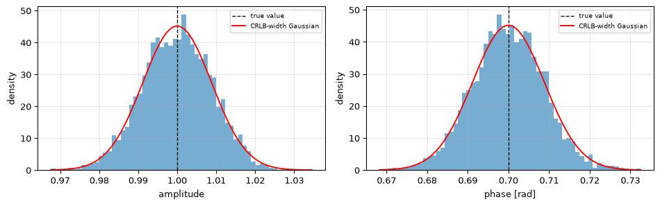
and the single-bin DFT attains both, at every \(N\), not merely asymptotically.
Integrate over whole cycles: what “coherent” is asking for
There is a condition attached, and it is easy to miss. The correlation above isolates the \(+f_0\) component only if the tone’s negative-frequency image at \(-f_0\) integrates to zero over the record, which happens exactly when the record spans a whole number of cycles, \(f_0 = k/N\) for integer \(k\). Otherwise a residue of the image leaks into the answer and biases both estimates by a term of order \(1/(N \sin 2\pi f_0)\): small, but deterministic, so no amount of averaging removes it. At \(N = 256\) and a tone sitting mid-bin, the phase bias is about 4 milliradians, roughly thirty times the standard error of a 4000-trial average.
This is why coherent instruments are built to control the ratio rather than tolerate it. The archive script behind this page runs at \(f_s = 16.0428\) kHz for a carrier of exactly \(f_s/58\): the sample rate was chosen so that a whole number of samples spans a whole number of cycles. Do the same where you can, and window the record where you cannot.
Show the code
rng = np.random.default_rng(4)A, phi, N, sigma =1.0, 0.7, 256, 0.1f0 =60/ N # whole number of cycles in the recordn = np.arange(N)amps, phases = [], []for _ inrange(4000): x = A * np.cos(2* np.pi * f0 * n + phi) + rng.normal(0, sigma, N) a, p = coherent_dft(x, f0) amps.append(a) phases.append(p)amps, phases = np.array(amps), np.array(phases)bound = crlb_known_frequency(A, sigma, N)fig, axes = plt.subplots(1, 2, figsize=(10, 3.2))for ax, data, truth, key, label in [ (axes[0], amps, A, 'amplitude', 'amplitude'), (axes[1], phases, phi, 'phase', 'phase [rad]')]: ax.hist(data, bins=60, density=True, alpha=0.6, color='C0') ax.axvline(truth, color='k', ls='--', lw=1, label='true value') grid = np.linspace(data.min(), data.max(), 200) ax.plot(grid, np.exp(-(grid - truth)**2/ (2* bound[key]))/ np.sqrt(2* np.pi * bound[key]), 'r-', lw=1.4, label='CRLB-width Gaussian') ax.set_xlabel(label); ax.set_ylabel('density') ax.legend(fontsize=7); ax.grid(True, alpha=0.3)fig.tight_layout(); plt.show()for name, data, truth, key in [('amplitude', amps, A, 'amplitude'), ('phase', phases, phi, 'phase')]: var, bias = data.var(), data.mean() - truthprint(f"{name:>9s}: bias {bias:+.2e}, var {var:.3e}, "f"CRLB {bound[key]:.3e}, ratio {var / bound[key]:.3f}")# 4000 trials give ~2.2% standard error on a variance; allow 10%.assertabs(var / bound[key] -1) <0.10, f"{name} should attain the bound"assertabs(bias) <4* np.sqrt(var /len(data)), f"{name} should be unbiased"# The callout's claim: move the same tone off-bin and a deterministic phase# bias appears, far larger than the standard error of the average.off = []for _ inrange(4000): x = A * np.cos(2* np.pi *0.2334* n + phi) + rng.normal(0, sigma, N) off.append(coherent_dft(x, 0.2334)[1])off = np.array(off)bias_off = off.mean() - phiprint(f"off-bin tone: phase bias {bias_off*1e3:+.2f} mrad, "f"{abs(bias_off)/np.sqrt(off.var()/len(off)):.0f}x its standard error")assertabs(bias_off) >20* np.sqrt(off.var() /len(off)), \"an off-bin tone should show a clearly significant phase bias"assertabs(bias_off) <0.01, "and it should still be small in absolute terms"
Figure 1: Coherent detection at a known frequency (N = 256, tone on bin 60, SNR 17 dB, 4000 trials). The amplitude and phase estimates are unbiased and their variances land on the Cramér-Rao bounds, so no estimator could do better with this data.
amplitude: bias +1.40e-05, var 7.798e-05, CRLB 7.813e-05, ratio 0.998
    phase: bias -9.52e-05, var 7.739e-05, CRLB 7.813e-05, ratio 0.991
off-bin tone: phase bias -4.24 mrad, 30x its standard error
Unknown frequency: the \(1/N^3\) law
Now let \(f_0\) be unknown too. The Cramér-Rao bound for the three-parameter problem (Rife and Boorstyn 1974) is where this page earns its keep:
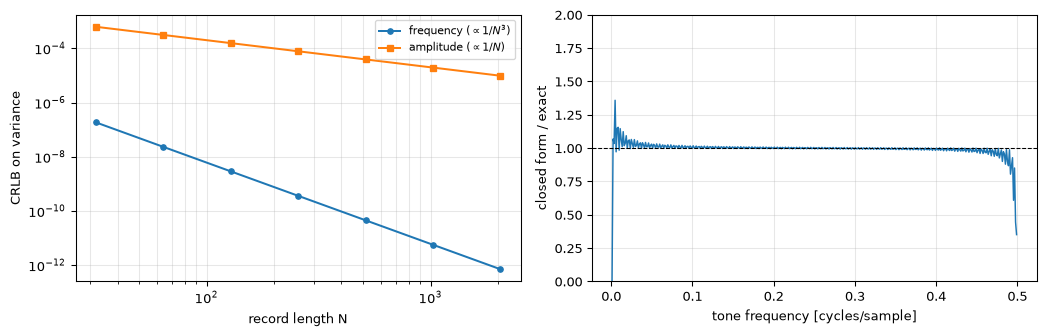
Look at the \(N\) dependence. Averaging, on the previous page, bought variance \(\propto 1/N\), so accuracy \(\propto 1/\sqrt{N}\): doubling the data bought a factor of 1.41. Here the variance falls as \(1/N^3\), so the standard deviation falls as \(N^{-3/2}\): doubling the record makes the frequency estimate 2.8 times more accurate. Ten times the data is a factor of 31.
The reason is worth internalising, because it recurs whenever you estimate a rate rather than a level. A longer record does two things at once. It averages down the noise, the familiar \(\sqrt{N}\). But it also extends the lever arm: a small frequency error accumulates into a phase error that grows linearly with time, so the longer you watch, the more visible a given frequency error becomes. The two effects multiply, and \(\sqrt{N} \times N = N^{3/2}\).
Two honest caveats attach to that formula, and both cost people real accuracy in practice.
Watch the parameterisation: where the factor of 2 hides
The constant 12 above is correct only when the bound is written in terms of the SNR \(\eta\). It is tempting to substitute \(\sigma^2/A^2\) for \(1/\eta\) and write \(12\sigma^2 / ((2\pi)^2 A^2 N(N^2-1))\). That is wrong by exactly a factor of two, because \(\eta = A^2/2\sigma^2\) carries the \(\tfrac{1}{2}\) from the cosine’s mean square. In terms of \(\sigma^2/A^2\) the constant is 24, not 12.
This is not a hypothetical: the substitution is the natural thing to write, it looks dimensionally fine, and no amount of re-reading the algebra reveals it. The only thing that catches it is checking the closed form against the exact Fisher information matrix computed numerically. It is a two-line check and it belongs in your workflow: the demo below runs it on every build, and test_snr_parameterisation_trap pins both forms so the mistake cannot come back.
The second caveat is that this closed form drops terms oscillating at \(2f_0\), which average away over a long record only when the tone is comfortably away from DC and Nyquist. Near either edge the approximation degrades sharply, and you should compute the exact bound instead.
Show the code
A, sigma =1.0, 0.1Ns = np.array([32, 64, 128, 256, 512, 1024, 2048])var_f = np.array([crlb_sinusoid(A, sigma, N)['frequency'] for N in Ns])var_A = np.array([crlb_sinusoid(A, sigma, N)['amplitude'] for N in Ns])fig, axes = plt.subplots(1, 2, figsize=(11, 3.6))axes[0].loglog(Ns, var_f, 'o-C0', ms=4, label=r'frequency ($\propto 1/N^3$)')axes[0].loglog(Ns, var_A, 's-C1', ms=4, label=r'amplitude ($\propto 1/N$)')axes[0].set_xlabel('record length N'); axes[0].set_ylabel('CRLB on variance')axes[0].legend(fontsize=8); axes[0].grid(True, which='both', alpha=0.3)f_grid = np.linspace(0.001, 0.499, 400)ratio = np.array([crlb_sinusoid(A, sigma, 256)['frequency']/ crlb_sinusoid_exact(A, 0.7, f, sigma, 256)['frequency']for f in f_grid])axes[1].plot(f_grid, ratio, 'C0', lw=1.1)axes[1].axhline(1.0, color='k', ls='--', lw=0.8)axes[1].set_xlabel('tone frequency [cycles/sample]')axes[1].set_ylabel('closed form / exact')axes[1].set_ylim(0, 2); axes[1].grid(True, alpha=0.3)fig.tight_layout(); plt.show()slope_f = np.polyfit(np.log(Ns), np.log(var_f), 1)[0]slope_A = np.polyfit(np.log(Ns), np.log(var_A), 1)[0]print(f"log-log slopes: frequency {slope_f:.3f} (theory -3), "f"amplitude {slope_A:.3f} (theory -1)")assertabs(slope_f +3) <0.05andabs(slope_A +1) <0.01# The closed form must track the exact FIM in the middle of the band...mid = (f_grid >0.05) & (f_grid <0.45)assert np.all(np.abs(ratio[mid] -1) <0.10), "closed form should hold mid-band"# ... and must visibly fail near the edges, as the caption claims.assert np.abs(ratio[f_grid <0.006] -1).max() >0.2, "should break near DC"# The parameterisation trap, checked on every build.eta = A**2/ (2* sigma**2)right =12/ ((2* np.pi)**2* eta *256* (256**2-1))wrong =12* sigma**2/ ((2* np.pi)**2* A**2*256* (256**2-1))exact = crlb_sinusoid_exact(A, 0.7, 0.23, sigma, 256)['frequency']print(f"SNR form {right:.4e} | sigma^2/A^2 form {wrong:.4e} "f"| exact FIM {exact:.4e}")assertabs(right / exact -1) <0.05, "the SNR form is the correct one"assertabs(right / wrong -2) <1e-9, "the naive substitution halves the bound"
Figure 2: Left: the frequency bound falls as 1/N³ (slope -3 on log-log), against 1/N for amplitude. Right: the large-N closed form matches the exact Fisher information across the middle of the band but breaks down within a few bins of DC and Nyquist, where the dropped 2f₀ terms stop averaging away.
log-log slopes: frequency -3.000 (theory -3), amplitude -1.000 (theory -1)
SNR form 3.6236e-10 | sigma^2/A^2 form 1.8118e-10 | exact FIM 3.6034e-10
Estimators: from the bin grid to the bound
The maximum likelihood estimate of \(f_0\) maximises the periodogram, so every practical estimator is a way of finding that peak cheaply.
The bare FFT peak takes the largest bin. Its resolution is the bin spacing \(f_s/N\), and that is a hard floor unrelated to noise: at high SNR the error stops improving because the answer is quantised to the grid. Zero-padding refines the grid but multiplies the FFT cost.
Interpolation uses the peak bin’s two neighbours to locate the true maximum between them, which is nearly free. Two standard choices are a parabola fitted to the log magnitudes, and the three-bin complex estimator of Jacobsen and Kootsookos (Jacobsen and Kootsookos 2007). (The same three-point move reappears on the lag axis in time-delay estimation, where the shape the parabola must match is the signal’s own autocorrelation peak.)
The phase-difference method splits the record in two, measures the phase of each half at the coarse peak frequency, and converts the phase advance between them into a frequency offset. It is the same principle as a phase-locked loop, and as the phase-vocoder refinement used in pitch detection.
Match the interpolator to the window
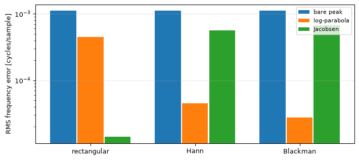
Both interpolators fit an assumed main-lobe shape, so using the wrong one leaves a bias that depends on where the tone falls inside its bin. Averaging never removes it, because it is not noise. Jacobsen’s estimator is derived for the rectangular window’s Dirichlet lobe; the log-parabola fits the near-Gaussian lobe of a tapered window. Getting the pairing backwards costs more than an order of magnitude, in either direction, as the demo below measures.
Show the code
rng = np.random.default_rng(1)N, sigma =256, 0.05windows = {'rectangular': np.ones(N), 'Hann': np.hanning(N),'Blackman': np.blackman(N)}modes = ('none', 'quadratic', 'jacobsen')rms = {w: {m: 0.0for m in modes} for w in windows}for wname, w in windows.items(): errs = {m: [] for m in modes}for i inrange(300): f_true = (20+ (i %97) /97.0) / N # sweep within one bin x = (np.cos(2* np.pi * f_true * np.arange(N) +0.7)+ rng.normal(0, sigma, N)) * wfor m in modes: errs[m].append(estimate_frequency_fft(x, interpolation=m) - f_true)for m in modes: rms[wname][m] =float(np.sqrt(np.mean(np.square(errs[m]))))fig, ax = plt.subplots(figsize=(7.5, 3.4))xpos = np.arange(len(windows))for j, m inenumerate(modes): ax.bar(xpos + (j -1) *0.26, [rms[w][m] for w in windows], 0.25, label={'none': 'bare peak', 'quadratic': 'log-parabola','jacobsen': 'Jacobsen'}[m])ax.set_yscale('log'); ax.set_xticks(xpos); ax.set_xticklabels(windows)ax.set_ylabel('RMS frequency error [cycles/sample]')ax.legend(fontsize=8); ax.grid(True, axis='y', alpha=0.3)fig.tight_layout(); plt.show()for w in windows:print(f"{w:>12s}: "+" ".join(f"{m}{rms[w][m]:.2e}"for m in modes))# The callout's claim, in both directions, with an order of magnitude to spare.assert rms['rectangular']['jacobsen'] < rms['rectangular']['quadratic'] /10for w in ('Hann', 'Blackman'):assert rms[w]['quadratic'] < rms[w]['jacobsen'] /10# The bare peak is grid-limited, so it beats neither at its own window.for w in windows:assert rms[w]['none'] >min(rms[w]['quadratic'], rms[w]['jacobsen'])
Figure 3: RMS frequency error over a swept fractional bin offset (N = 256, SNR 23 dB, 97 sub-bin offsets over 300 trials). Jacobsen’s estimator suits the rectangular window and the log-parabola suits tapered windows; each is roughly an order of magnitude worse on the other’s window. The bare peak is limited by the bin grid regardless.
Here is the behaviour that separates frequency estimation from everything on the previous page. Sweep the SNR and watch a periodogram-based estimator against the bound.
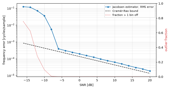
Above a threshold, the estimator tracks the CRLB at a constant offset: the peak it finds is the right peak, and only its exact position is uncertain, so the error falls in step with the bound as the noise drops. Below the threshold, noise occasionally produces a taller peak somewhere else entirely, and the estimate is not slightly wrong but wildly wrong, off by many bins. The error distribution stops being a tight bell and becomes a mixture: mostly good estimates, plus a growing fraction of essentially random ones. RMS error, which averages the squares, is dominated by those outliers and rockets away from the bound (Rife and Boorstyn 1974).
The constant offset above threshold is worth reading correctly, because it is not the threshold effect and not a failure of the theory. The Jacobsen estimator sits at about 1.4 times the bound across the whole usable range: that gap is the price of locating the peak from three bins instead of maximising the periodogram properly. Refining the peak by direct numerical maximisation closes it to within a few percent of the bound (measured: 1.05 to 1.09 times, against Jacobsen’s 1.43), at considerably more arithmetic. Whether that last 40% is worth an iterative search is a cycle-budget question, and on a microcontroller the answer is usually no: the embedded companion shows why the three-bin form is what ships.
Show the code
rng = np.random.default_rng(7)N, A, f_true =256, 1.0, 0.2334snr_db = np.arange(-16, 21, 2)n = np.arange(N)rmse, bound_std, outlier_frac = [], [], []for s_db in snr_db: eta =10** (s_db /10) sigma = np.sqrt(A**2/ (2* eta)) est = np.array([ estimate_frequency_fft(A * np.cos(2* np.pi * f_true * n +0.7)+ rng.normal(0, sigma, N), interpolation='jacobsen')for _ inrange(400)]) err = est - f_true rmse.append(np.sqrt(np.mean(err**2))) outlier_frac.append(np.mean(np.abs(err) >1.0/ N)) # >1 bin off bound_std.append(np.sqrt(crlb_sinusoid(A, sigma, N)['frequency']))rmse, bound_std, outlier_frac =map(np.array, (rmse, bound_std, outlier_frac))fig, ax = plt.subplots(figsize=(7.5, 4))ax.semilogy(snr_db, rmse, 'o-C0', ms=4, label='Jacobsen estimator, RMS error')ax.semilogy(snr_db, bound_std, 'k--', lw=1.2, label='Cramér-Rao bound')ax.set_xlabel('SNR [dB]'); ax.set_ylabel('frequency error [cycles/sample]')ax.grid(True, which='both', alpha=0.3)ax2 = ax.twinx()ax2.plot(snr_db, outlier_frac, ':C3', lw=1.4, label='fraction > 1 bin off')ax2.set_ylabel('outlier fraction', color='C3'); ax2.set_ylim(0, 1)lines = ax.get_lines() + ax2.get_lines()ax.legend(lines, [l.get_label() for l in lines], fontsize=8, loc='upper right')fig.tight_layout(); plt.show()ratio = rmse / bound_stdfor s, r, o inzip(snr_db, ratio, outlier_frac):print(f"SNR {s:+3d} dB: RMS/CRLB {r:8.2f}, outliers {o*100:5.1f}%")high = snr_db >=-6# above thresholdlow = snr_db <=-12# below it# Above threshold the estimator tracks the bound at a near-constant offset:# the ratio is flat, so the error falls with the bound as the noise drops.assert np.all(ratio[high] <2.0), "should track the bound above threshold"assert ratio[high].max() / ratio[high].min() <1.2, "offset should be flat"assert outlier_frac[high].max() ==0.0, "no outliers above threshold"# Below it, the ratio explodes and outliers take over.assert ratio[low].min() >50, "should depart badly below threshold"assert outlier_frac[low].min() >0.25, "outliers should be common below threshold"print(f"\nabove threshold: RMS/CRLB flat at {ratio[high].mean():.2f} "f"(the interpolator's own loss); below: up to {ratio[low].max():.0f}")
Figure 4: The threshold effect (N = 256, 400 trials per point). Above about -7 dB SNR the estimator tracks the Cramér-Rao bound at a constant offset, falling with it as the noise drops. Below that, noise starts winning the peak competition outright and the RMS error departs by two orders of magnitude. The dotted line shows the fraction of estimates landing more than one bin from the truth: these outliers, not a gentle loss of precision, are what breaks the estimator.
The practical consequences are worth stating plainly, because they contradict the intuition the \(\sqrt{N}\) world trains:
Averaging estimates does not rescue you below threshold. The outliers are not zero-mean perturbations, they are draws from a nearly uniform distribution across the band. Averaging a good estimate with a random one gives a mediocre estimate. Take a longer record, or filter first.
Threshold SNR moves with \(N\), because a longer record concentrates the tone into a narrower peak while the noise floor stays put. Buying record length buys threshold margin as well as precision.
Report the outlier rate, not just the RMS error. An estimator quoted at “3% RMS” might be right to 0.1% nine times in ten and useless the tenth. The ROC-style thinking applies here too: a single summary number hides a mixture.
Efficient does not mean unbiased
Above threshold the periodogram maximiser is efficient in variance: measured against the bound at 16 dB SNR its standard deviation is within a couple of percent. But it retains a small deterministic bias, visible even with the noise switched off entirely, because a real tone’s negative-frequency image at \(-f_0\) pulls slightly on the peak at \(+f_0\). The bias decays with record length (measured at \(2.0 \times 10^{-4}\) cycles/sample at \(N=64\), falling to \(9.2 \times 10^{-7}\) at \(N=1024\)) and is negligible whenever the tone is many bins from DC. It is worth knowing about because the Cramér-Rao bound says nothing about it: the bound constrains unbiased estimators, so a bias floor can and does sit underneath a variance that looks perfectly efficient.
A war story: calibrating a detector by sweeping it
The archive behind this page includes a measurement script from an FPGA-based instrument that is a nice illustration of using the theory instead of brute force.
The instrument performed synchronous detection in hardware: multiply the incoming signal by a reference at the known frequency, integrate, read out a number. That number depends on the phase of the reference relative to the signal, and it is maximised when the two are aligned. Since the relative phase depended on cable lengths and analogue delays, it had to be calibrated per setup: find the reference phase that maximises the detector output.
The obvious approach is to hill-climb, nudging the phase and keeping the changes that increase the output. On a noisy hardware measurement that is slow and unreliable, and it stalls on local wobbles.
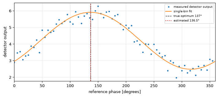
What the script does instead: sweep the detection phase across a full turn, recording the detector output at each step, then take the DFT of that record and read the answer off the phase of bin 1. Because the detector’s response to a phase offset is itself a cosine of exactly one cycle per turn, the optimal phase is the argument of the single DFT bin at one cycle per sweep. One sweep, one inner product, no iteration, and all the noise in the other bins is rejected by construction.
It is the same single-bin DFT from the top of this page, turned on the instrument itself. Estimation theory says a coherent detector is the optimal way to measure the amplitude and phase of a known-frequency sinusoid; here the “signal” is the calibration sweep, and the “known frequency” is one cycle per sweep, guaranteed by how you swept it. Recognising a measurement problem as an instance of a solved estimation problem is most of the value of a page like this one.
Show the code
rng = np.random.default_rng(11)n_steps =72true_opt_deg =137.0sweep_deg = np.arange(n_steps) *360.0/ n_steps# A synchronous detector's output vs reference phase is a cosine peaking# at the aligned phase, plus measurement noise and an arbitrary offset.detector =4.2+1.8* np.cos(np.radians(sweep_deg - true_opt_deg))measured = detector + rng.normal(0, 0.35, n_steps)# One bin, one cycle per sweep. Exactly coherent_dft with f0 = 1/n_steps.# Mind the sign: coherent_dft models A*cos(2*pi*f0*n + phase), while the# sweep is cos(2*pi*n/n_steps - opt), so the optimum is minus the# reported phase._, phase = coherent_dft(measured - measured.mean(), 1.0/ n_steps)est_opt_deg = (-np.degrees(phase)) %360.0fig, ax = plt.subplots(figsize=(7.5, 3.4))ax.plot(sweep_deg, measured, '.C0', ms=5, label='measured detector output')fine = np.linspace(0, 360, 400)ax.plot(fine, measured.mean() + np.abs(np.mean( (measured - measured.mean()) * np.exp(-2j* np.pi * np.arange(n_steps) / n_steps))) *2* np.cos(np.radians(fine - est_opt_deg)), 'C1', lw=1.4, label='single-bin fit')ax.axvline(true_opt_deg, color='k', ls='--', lw=1, label=f'true optimum {true_opt_deg:.0f}°')ax.axvline(est_opt_deg, color='C3', ls=':', lw=1.6, label=f'estimated {est_opt_deg:.1f}°')ax.set_xlabel('reference phase [degrees]'); ax.set_ylabel('detector output')ax.set_xlim(0, 360); ax.legend(fontsize=7); ax.grid(True, alpha=0.3)fig.tight_layout(); plt.show()err = (est_opt_deg - true_opt_deg +180) %360-180best_sample = sweep_deg[np.argmax(measured)]err_argmax = (best_sample - true_opt_deg +180) %360-180# What is achievable here: the sweep is a known-frequency tone (one cycle# per sweep by construction), so the known-frequency phase bound applies.bound_deg = np.degrees(np.sqrt(crlb_known_frequency(1.8, 0.35, n_steps)['phase']))print(f"single-bin DFT estimate: {est_opt_deg:.2f}°, error {err:+.2f}°")print(f"just taking the largest sample: {best_sample:.1f}°, error {err_argmax:+.1f}°")print(f"Cramer-Rao bound on the phase at this SNR and sweep length: {bound_deg:.1f}°")# The caption's claims. Note the threshold is one bound-width, not tighter:# the estimator sits ON the bound, so demanding much better than 1.9 deg# would be demanding the impossible, however tempting the seeded run looks.assert1.8< bound_deg <2.0, f"expected a ~1.9 deg bound, got {bound_deg:.2f}"assertabs(err) <2.0, "the one-bin estimate should land within about the bound"assertabs(err) <abs(err_argmax) /3, "and be several times better than the argmax"
Figure 5: The calibration trick, simulated. A synchronous detector’s output is swept across all reference phases (noisy dots). Rather than hill-climbing, one DFT bin at exactly one cycle per sweep recovers the optimal phase to within a degree or two, using every sample in the sweep and rejecting the noise in every other bin. The known-frequency phase bound at this sweep length and SNR is 1.9 degrees, so that is about as well as any method could do here; picking the single largest reading is several times worse.
single-bin DFT estimate: 136.47°, error -0.53°
just taking the largest sample: 150.0°, error +13.0°
Cramer-Rao bound on the phase at this SNR and sweep length: 1.9°
Picking the largest measured sample, the naive alternative, is limited both by the sweep step and by the noise on that one reading. The single-bin estimate uses all of them.
On hardware
A tone tracker is one of the most useful things a microcontroller can do, and one of the cheapest: a Goertzel filter or a small FFT, a peak interpolation, and you have an instrument. The embedded companion builds it on both default platforms, including the fixed-point and cycle-budget consequences of everything above.
Going further
Multiple tones. Everything here assumed a single sinusoid. Two tones closer than about one bin apart interfere in the periodogram, and their individual parameters become poorly determined no matter how good your peak-finding is: the bound itself degrades. Rife and Boorstyn extended the analysis to multiple tones, and the subspace methods (MUSIC, ESPRIT) attack the same problem by a different route, as the beamforming page’s adaptive section notes in the spatial domain.
Tones that drift. A frequency that changes during the record breaks the model, and the \(1/N^3\) law stops rewarding longer records: past some length you are averaging over a frequency that has moved. The practical answer is the STFT, which trades the \(N^{3/2}\) gain for the ability to track, and the honest question is where to set that trade for your signal.
Estimators that beat the threshold. The threshold is a property of the periodogram-maximising approach, not a law of nature. Below it, methods that exploit additional structure (a known modulation, a phase-locked loop with a good initial estimate, or a Bayesian prior on where the tone can be) still work where the peak-picker fails. This is where the frequentist framing of estimation basics starts to strain, and prior information stops being a luxury.
References
Jacobsen, Eric, and Peter Kootsookos. 2007. “Fast, Accurate Frequency Estimators [DSP Tips & Tricks].”IEEE Signal Processing Magazine 24 (3): 123–25. https://doi.org/10.1109/MSP.2007.361611.
Rife, David C., and Robert R. Boorstyn. 1974. “Single-Tone Parameter Estimation from Discrete-Time Observations.”IEEE Transactions on Information Theory 20 (5): 591–98. https://doi.org/10.1109/TIT.1974.1055282.
Source Code
---title: "Estimating a Sinusoid"subtitle: "Amplitude, phase, and frequency of a tone in noise"description-meta: "Amplitude, phase and frequency of a tone in noise: the periodogram peak, its interpolation, and the Cramer-Rao bound on how well you can do."bibliography: ../../references.bib---A tone in noise is the most-measured signal in engineering. A guitar string, a rotating shaft's vibration line, a radar return, a lock-in amplifier's carrier, a power line at 50 Hz, an ultrasonic ranging burst: all of them reduce to "there is a sinusoid in here, tell me about it".The signal has three parameters, and they behave so differently that a single page comparing them is worth more than three pages treating them separately. **Amplitude and phase** are easy in a precise sense: given the frequency, the model is linear in them, so the best possible estimator is a single inner product, and it reaches the theoretical limit exactly. **Frequency** is not linear in anything, and it rewards a longer record far more generously than averaging ever does: its accuracy improves with the *cube* of the record length. It also has a cliff. Below a threshold signal-to-noise ratio, every frequency estimator stops degrading gracefully and simply breaks.::: {.callout-note title="Prerequisites"}Part of the [estimation & detection arc](../estimation-and-detection.qmd); the overview gives the reading order.[Estimation basics](../estimation-basics/index.qmd) (bias, variance, the Cramér-Rao bound, maximum likelihood) is the companion page; this one is its first real application. You will also want [the frequency domain](../../basics/05-frequency-domain.qmd) (DFT, bins, leakage, windows) and [noise and SNR](../../basics/03-noise-snr.qmd).:::::: {.callout-tip title="Code"}The implementation is [`sinusoid.py`](sinusoid.py). Save [`test_sinusoid.py`](test_sinusoid.py) beside it and `pytest test_sinusoid.py` runs the checks on it.:::```{python}#| echo: falseimport numpy as npimport matplotlib.pyplot as pltfrom sinusoid import (coherent_dft, crlb_sinusoid, crlb_sinusoid_exact, crlb_known_frequency, estimate_frequency_fft, estimate_frequency_phase_diff)```<hr>## The model, and why the frequency is the hard oneThroughout, the signal is a real tone in white Gaussian noise:$$x[n] = A \cos(2\pi f_0 n + \phi) + w[n], \qquad w[n] \sim \mathcal{N}(0, \sigma^2), \qquad n = 0, \ldots, N-1$$with $f_0$ in cycles per sample. The natural measure of signal quality is the signal-to-noise ratio, the tone's power over the noise power:$$\eta = \frac{A^2/2}{\sigma^2} = \frac{A^2}{2\sigma^2}$$That factor of $\tfrac{1}{2}$ (a cosine of amplitude $A$ has mean square $A^2/2$, not $A^2$) is going to matter more than it looks. Hold onto it.Why is frequency structurally different? Write the signal as $A\cos\phi \cos(2\pi f_0 n) - A\sin\phi \sin(2\pi f_0 n)$. For a *known* $f_0$ this is a linear combination of two known basis sequences with coefficients $A\cos\phi$ and $-A\sin\phi$: exactly the linear model from [estimation basics](../estimation-basics/index.qmd#prior-knowledge-beats-more-data-weighted-least-squares), where least squares is optimal and attains the bound. But $f_0$ sits *inside* the basis functions. Changing it does not rescale the model, it reshapes it. That single fact is the source of everything unusual below.<hr>## Known frequency: the coherent single-bin DFTWhen you already know the frequency (a lock-in amplifier drives its own reference; a power monitor knows it is looking for 50 Hz), estimating amplitude and phase is a projection. Correlate the record against a complex exponential at $f_0$:$$z = \frac{1}{N}\sum_{n=0}^{N-1} x[n]\, e^{-j 2\pi f_0 n}, \qquad \hat{A} = 2|z|, \qquad \hat{\phi} = \arg z$$This is the **single-bin DFT**: one bin of a DFT you never fully compute. It is simultaneously the maximum likelihood estimator of amplitude and phase, the matched filter for a tone, what [a lock-in amplifier](../lock-in-detection/index.qmd) does in analogue hardware, and what [the Goertzel algorithm](../goertzel/index.qmd) computes recursively when you want it sample by sample instead of block by block. The factor of two is real-signal bookkeeping: a real cosine splits its energy between $+f_0$ and $-f_0$, so a single-sided correlation recovers $A/2$.The Cramér-Rao bounds for this two-parameter problem are$$\operatorname{var}(\hat{A}) \ge \frac{2\sigma^2}{N}, \qquad \operatorname{var}(\hat{\phi}) \ge \frac{1}{\eta N}$$and the single-bin DFT attains both, at every $N$, not merely asymptotically.::: {.callout-tip title="Integrate over whole cycles: what \"coherent\" is asking for"}There is a condition attached, and it is easy to miss. The correlation above isolates the $+f_0$ component only if the tone's negative-frequency image at $-f_0$ integrates to zero over the record, which happens exactly when the record spans a whole number of cycles, $f_0 = k/N$ for integer $k$. Otherwise a residue of the image leaks into the answer and biases both estimates by a term of order $1/(N \sin 2\pi f_0)$: small, but deterministic, so no amount of averaging removes it. At $N = 256$ and a tone sitting mid-bin, the phase bias is about 4 milliradians, roughly thirty times the standard error of a 4000-trial average.This is why coherent instruments are built to control the ratio rather than tolerate it. The archive script behind this page runs at $f_s = 16.0428$ kHz for a carrier of exactly $f_s/58$: the sample rate was *chosen* so that a whole number of samples spans a whole number of cycles. Do the same where you can, and window the record where you cannot.:::```{python}#| label: fig-coherent#| fig-cap: "Coherent detection at a known frequency (N = 256, tone on bin 60, SNR 17 dB, 4000 trials). The amplitude and phase estimates are unbiased and their variances land on the Cramér-Rao bounds, so no estimator could do better with this data."rng = np.random.default_rng(4)A, phi, N, sigma =1.0, 0.7, 256, 0.1f0 =60/ N # whole number of cycles in the recordn = np.arange(N)amps, phases = [], []for _ inrange(4000): x = A * np.cos(2* np.pi * f0 * n + phi) + rng.normal(0, sigma, N) a, p = coherent_dft(x, f0) amps.append(a) phases.append(p)amps, phases = np.array(amps), np.array(phases)bound = crlb_known_frequency(A, sigma, N)fig, axes = plt.subplots(1, 2, figsize=(10, 3.2))for ax, data, truth, key, label in [ (axes[0], amps, A, 'amplitude', 'amplitude'), (axes[1], phases, phi, 'phase', 'phase [rad]')]: ax.hist(data, bins=60, density=True, alpha=0.6, color='C0') ax.axvline(truth, color='k', ls='--', lw=1, label='true value') grid = np.linspace(data.min(), data.max(), 200) ax.plot(grid, np.exp(-(grid - truth)**2/ (2* bound[key]))/ np.sqrt(2* np.pi * bound[key]), 'r-', lw=1.4, label='CRLB-width Gaussian') ax.set_xlabel(label); ax.set_ylabel('density') ax.legend(fontsize=7); ax.grid(True, alpha=0.3)fig.tight_layout(); plt.show()for name, data, truth, key in [('amplitude', amps, A, 'amplitude'), ('phase', phases, phi, 'phase')]: var, bias = data.var(), data.mean() - truthprint(f"{name:>9s}: bias {bias:+.2e}, var {var:.3e}, "f"CRLB {bound[key]:.3e}, ratio {var / bound[key]:.3f}")# 4000 trials give ~2.2% standard error on a variance; allow 10%.assertabs(var / bound[key] -1) <0.10, f"{name} should attain the bound"assertabs(bias) <4* np.sqrt(var /len(data)), f"{name} should be unbiased"# The callout's claim: move the same tone off-bin and a deterministic phase# bias appears, far larger than the standard error of the average.off = []for _ inrange(4000): x = A * np.cos(2* np.pi *0.2334* n + phi) + rng.normal(0, sigma, N) off.append(coherent_dft(x, 0.2334)[1])off = np.array(off)bias_off = off.mean() - phiprint(f"off-bin tone: phase bias {bias_off*1e3:+.2f} mrad, "f"{abs(bias_off)/np.sqrt(off.var()/len(off)):.0f}x its standard error")assertabs(bias_off) >20* np.sqrt(off.var() /len(off)), \"an off-bin tone should show a clearly significant phase bias"assertabs(bias_off) <0.01, "and it should still be small in absolute terms"```<hr>## Unknown frequency: the $1/N^3$ lawNow let $f_0$ be unknown too. The Cramér-Rao bound for the three-parameter problem [@rife1974single] is where this page earns its keep:$$\operatorname{var}(\hat{f_0}) \ge \frac{12}{(2\pi)^2\, \eta\, N(N^2-1)} \;\approx\; \frac{3}{\pi^2 \eta N^3} \quad \text{for large } N$$Look at the $N$ dependence. Averaging, on [the previous page](../estimation-basics/index.qmd#consistency-and-why-averaging-buys-sqrtn), bought variance $\propto 1/N$, so accuracy $\propto 1/\sqrt{N}$: doubling the data bought a factor of 1.41. Here the variance falls as $1/N^3$, so the standard deviation falls as $N^{-3/2}$: **doubling the record makes the frequency estimate 2.8 times more accurate**. Ten times the data is a factor of 31.The reason is worth internalising, because it recurs whenever you estimate a rate rather than a level. A longer record does two things at once. It averages down the noise, the familiar $\sqrt{N}$. But it also *extends the lever arm*: a small frequency error accumulates into a phase error that grows linearly with time, so the longer you watch, the more visible a given frequency error becomes. The two effects multiply, and $\sqrt{N} \times N = N^{3/2}$.Two honest caveats attach to that formula, and both cost people real accuracy in practice.::: {.callout-warning title="Watch the parameterisation: where the factor of 2 hides"}The constant 12 above is correct **only when the bound is written in terms of the SNR $\eta$**. It is tempting to substitute $\sigma^2/A^2$ for $1/\eta$ and write $12\sigma^2 / ((2\pi)^2 A^2 N(N^2-1))$. That is wrong by exactly a factor of two, because $\eta = A^2/2\sigma^2$ carries the $\tfrac{1}{2}$ from the cosine's mean square. In terms of $\sigma^2/A^2$ the constant is **24**, not 12.This is not a hypothetical: the substitution is the natural thing to write, it looks dimensionally fine, and no amount of re-reading the algebra reveals it. The only thing that catches it is checking the closed form against the exact Fisher information matrix computed numerically. It is a two-line check and it belongs in your workflow: the demo below runs it on every build, and `test_snr_parameterisation_trap` pins both forms so the mistake cannot come back.:::The second caveat is that this closed form drops terms oscillating at $2f_0$, which average away over a long record only when the tone is comfortably away from DC and Nyquist. Near either edge the approximation degrades sharply, and you should compute the exact bound instead.```{python}#| label: fig-crlb#| fig-cap: "Left: the frequency bound falls as 1/N³ (slope -3 on log-log), against 1/N for amplitude. Right: the large-N closed form matches the exact Fisher information across the middle of the band but breaks down within a few bins of DC and Nyquist, where the dropped 2f₀ terms stop averaging away."A, sigma =1.0, 0.1Ns = np.array([32, 64, 128, 256, 512, 1024, 2048])var_f = np.array([crlb_sinusoid(A, sigma, N)['frequency'] for N in Ns])var_A = np.array([crlb_sinusoid(A, sigma, N)['amplitude'] for N in Ns])fig, axes = plt.subplots(1, 2, figsize=(11, 3.6))axes[0].loglog(Ns, var_f, 'o-C0', ms=4, label=r'frequency ($\propto 1/N^3$)')axes[0].loglog(Ns, var_A, 's-C1', ms=4, label=r'amplitude ($\propto 1/N$)')axes[0].set_xlabel('record length N'); axes[0].set_ylabel('CRLB on variance')axes[0].legend(fontsize=8); axes[0].grid(True, which='both', alpha=0.3)f_grid = np.linspace(0.001, 0.499, 400)ratio = np.array([crlb_sinusoid(A, sigma, 256)['frequency']/ crlb_sinusoid_exact(A, 0.7, f, sigma, 256)['frequency']for f in f_grid])axes[1].plot(f_grid, ratio, 'C0', lw=1.1)axes[1].axhline(1.0, color='k', ls='--', lw=0.8)axes[1].set_xlabel('tone frequency [cycles/sample]')axes[1].set_ylabel('closed form / exact')axes[1].set_ylim(0, 2); axes[1].grid(True, alpha=0.3)fig.tight_layout(); plt.show()slope_f = np.polyfit(np.log(Ns), np.log(var_f), 1)[0]slope_A = np.polyfit(np.log(Ns), np.log(var_A), 1)[0]print(f"log-log slopes: frequency {slope_f:.3f} (theory -3), "f"amplitude {slope_A:.3f} (theory -1)")assertabs(slope_f +3) <0.05andabs(slope_A +1) <0.01# The closed form must track the exact FIM in the middle of the band...mid = (f_grid >0.05) & (f_grid <0.45)assert np.all(np.abs(ratio[mid] -1) <0.10), "closed form should hold mid-band"# ... and must visibly fail near the edges, as the caption claims.assert np.abs(ratio[f_grid <0.006] -1).max() >0.2, "should break near DC"# The parameterisation trap, checked on every build.eta = A**2/ (2* sigma**2)right =12/ ((2* np.pi)**2* eta *256* (256**2-1))wrong =12* sigma**2/ ((2* np.pi)**2* A**2*256* (256**2-1))exact = crlb_sinusoid_exact(A, 0.7, 0.23, sigma, 256)['frequency']print(f"SNR form {right:.4e} | sigma^2/A^2 form {wrong:.4e} "f"| exact FIM {exact:.4e}")assertabs(right / exact -1) <0.05, "the SNR form is the correct one"assertabs(right / wrong -2) <1e-9, "the naive substitution halves the bound"```<hr>## Estimators: from the bin grid to the boundThe maximum likelihood estimate of $f_0$ maximises the periodogram, so every practical estimator is a way of finding that peak cheaply.**The bare FFT peak** takes the largest bin. Its resolution is the bin spacing $f_s/N$, and that is a hard floor unrelated to noise: at high SNR the error stops improving because the answer is quantised to the grid. Zero-padding refines the grid but multiplies the FFT cost.**Interpolation** uses the peak bin's two neighbours to locate the true maximum between them, which is nearly free. Two standard choices are a parabola fitted to the log magnitudes, and the three-bin complex estimator of Jacobsen and Kootsookos [@jacobsen2007fast]. (The same three-point move reappears on the *lag* axis in [time-delay estimation](../time-delay-estimation/index.qmd#reading-the-peak-off-the-grid), where the shape the parabola must match is the signal's own autocorrelation peak.)**The phase-difference method** splits the record in two, measures the phase of each half at the coarse peak frequency, and converts the phase advance between them into a frequency offset. It is the same principle as a phase-locked loop, and as the phase-vocoder refinement used in [pitch detection](../pitch-detection/index.qmd).::: {.callout-important title="Match the interpolator to the window"}Both interpolators fit an assumed main-lobe shape, so using the wrong one leaves a bias that depends on where the tone falls inside its bin. Averaging never removes it, because it is not noise. Jacobsen's estimator is derived for the rectangular window's Dirichlet lobe; the log-parabola fits the near-Gaussian lobe of a tapered window. Getting the pairing backwards costs more than an order of magnitude, in *either* direction, as the demo below measures.:::```{python}#| label: fig-interpolators#| fig-cap: "RMS frequency error over a swept fractional bin offset (N = 256, SNR 23 dB, 97 sub-bin offsets over 300 trials). Jacobsen's estimator suits the rectangular window and the log-parabola suits tapered windows; each is roughly an order of magnitude worse on the other's window. The bare peak is limited by the bin grid regardless."rng = np.random.default_rng(1)N, sigma =256, 0.05windows = {'rectangular': np.ones(N), 'Hann': np.hanning(N),'Blackman': np.blackman(N)}modes = ('none', 'quadratic', 'jacobsen')rms = {w: {m: 0.0for m in modes} for w in windows}for wname, w in windows.items(): errs = {m: [] for m in modes}for i inrange(300): f_true = (20+ (i %97) /97.0) / N # sweep within one bin x = (np.cos(2* np.pi * f_true * np.arange(N) +0.7)+ rng.normal(0, sigma, N)) * wfor m in modes: errs[m].append(estimate_frequency_fft(x, interpolation=m) - f_true)for m in modes: rms[wname][m] =float(np.sqrt(np.mean(np.square(errs[m]))))fig, ax = plt.subplots(figsize=(7.5, 3.4))xpos = np.arange(len(windows))for j, m inenumerate(modes): ax.bar(xpos + (j -1) *0.26, [rms[w][m] for w in windows], 0.25, label={'none': 'bare peak', 'quadratic': 'log-parabola','jacobsen': 'Jacobsen'}[m])ax.set_yscale('log'); ax.set_xticks(xpos); ax.set_xticklabels(windows)ax.set_ylabel('RMS frequency error [cycles/sample]')ax.legend(fontsize=8); ax.grid(True, axis='y', alpha=0.3)fig.tight_layout(); plt.show()for w in windows:print(f"{w:>12s}: "+" ".join(f"{m}{rms[w][m]:.2e}"for m in modes))# The callout's claim, in both directions, with an order of magnitude to spare.assert rms['rectangular']['jacobsen'] < rms['rectangular']['quadratic'] /10for w in ('Hann', 'Blackman'):assert rms[w]['quadratic'] < rms[w]['jacobsen'] /10# The bare peak is grid-limited, so it beats neither at its own window.for w in windows:assert rms[w]['none'] >min(rms[w]['quadratic'], rms[w]['jacobsen'])```<hr>## The cliff: threshold SNRHere is the behaviour that separates frequency estimation from everything on the previous page. Sweep the SNR and watch a periodogram-based estimator against the bound.Above a threshold, the estimator tracks the CRLB at a constant offset: the peak it finds is the right peak, and only its exact position is uncertain, so the error falls in step with the bound as the noise drops. Below the threshold, noise occasionally produces a *taller* peak somewhere else entirely, and the estimate is not slightly wrong but wildly wrong, off by many bins. The error distribution stops being a tight bell and becomes a mixture: mostly good estimates, plus a growing fraction of essentially random ones. RMS error, which averages the squares, is dominated by those outliers and rockets away from the bound [@rife1974single].The constant offset above threshold is worth reading correctly, because it is not the threshold effect and not a failure of the theory. The Jacobsen estimator sits at about 1.4 times the bound across the whole usable range: that gap is the price of locating the peak from three bins instead of maximising the periodogram properly. Refining the peak by direct numerical maximisation closes it to within a few percent of the bound (measured: 1.05 to 1.09 times, against Jacobsen's 1.43), at considerably more arithmetic. Whether that last 40% is worth an iterative search is a cycle-budget question, and on a microcontroller the answer is usually no: the [embedded companion](embedded.qmd) shows why the three-bin form is what ships.```{python}#| label: fig-threshold#| fig-cap: "The threshold effect (N = 256, 400 trials per point). Above about -7 dB SNR the estimator tracks the Cramér-Rao bound at a constant offset, falling with it as the noise drops. Below that, noise starts winning the peak competition outright and the RMS error departs by two orders of magnitude. The dotted line shows the fraction of estimates landing more than one bin from the truth: these outliers, not a gentle loss of precision, are what breaks the estimator."rng = np.random.default_rng(7)N, A, f_true =256, 1.0, 0.2334snr_db = np.arange(-16, 21, 2)n = np.arange(N)rmse, bound_std, outlier_frac = [], [], []for s_db in snr_db: eta =10** (s_db /10) sigma = np.sqrt(A**2/ (2* eta)) est = np.array([ estimate_frequency_fft(A * np.cos(2* np.pi * f_true * n +0.7)+ rng.normal(0, sigma, N), interpolation='jacobsen')for _ inrange(400)]) err = est - f_true rmse.append(np.sqrt(np.mean(err**2))) outlier_frac.append(np.mean(np.abs(err) >1.0/ N)) # >1 bin off bound_std.append(np.sqrt(crlb_sinusoid(A, sigma, N)['frequency']))rmse, bound_std, outlier_frac =map(np.array, (rmse, bound_std, outlier_frac))fig, ax = plt.subplots(figsize=(7.5, 4))ax.semilogy(snr_db, rmse, 'o-C0', ms=4, label='Jacobsen estimator, RMS error')ax.semilogy(snr_db, bound_std, 'k--', lw=1.2, label='Cramér-Rao bound')ax.set_xlabel('SNR [dB]'); ax.set_ylabel('frequency error [cycles/sample]')ax.grid(True, which='both', alpha=0.3)ax2 = ax.twinx()ax2.plot(snr_db, outlier_frac, ':C3', lw=1.4, label='fraction > 1 bin off')ax2.set_ylabel('outlier fraction', color='C3'); ax2.set_ylim(0, 1)lines = ax.get_lines() + ax2.get_lines()ax.legend(lines, [l.get_label() for l in lines], fontsize=8, loc='upper right')fig.tight_layout(); plt.show()ratio = rmse / bound_stdfor s, r, o inzip(snr_db, ratio, outlier_frac):print(f"SNR {s:+3d} dB: RMS/CRLB {r:8.2f}, outliers {o*100:5.1f}%")high = snr_db >=-6# above thresholdlow = snr_db <=-12# below it# Above threshold the estimator tracks the bound at a near-constant offset:# the ratio is flat, so the error falls with the bound as the noise drops.assert np.all(ratio[high] <2.0), "should track the bound above threshold"assert ratio[high].max() / ratio[high].min() <1.2, "offset should be flat"assert outlier_frac[high].max() ==0.0, "no outliers above threshold"# Below it, the ratio explodes and outliers take over.assert ratio[low].min() >50, "should depart badly below threshold"assert outlier_frac[low].min() >0.25, "outliers should be common below threshold"print(f"\nabove threshold: RMS/CRLB flat at {ratio[high].mean():.2f} "f"(the interpolator's own loss); below: up to {ratio[low].max():.0f}")```The practical consequences are worth stating plainly, because they contradict the intuition the $\sqrt{N}$ world trains:- **Averaging estimates does not rescue you below threshold.** The outliers are not zero-mean perturbations, they are draws from a nearly uniform distribution across the band. Averaging a good estimate with a random one gives a mediocre estimate. Take a longer record, or filter first.- **Threshold SNR moves with $N$**, because a longer record concentrates the tone into a narrower peak while the noise floor stays put. Buying record length buys threshold margin as well as precision.- **Report the outlier rate, not just the RMS error.** An estimator quoted at "3% RMS" might be right to 0.1% nine times in ten and useless the tenth. The [ROC-style thinking](../outlier-detection/index.qmd#which-detector-at-which-threshold-the-roc-curve) applies here too: a single summary number hides a mixture.::: {.callout-note title="Efficient does not mean unbiased"}Above threshold the periodogram maximiser is efficient in *variance*: measured against the bound at 16 dB SNR its standard deviation is within a couple of percent. But it retains a small deterministic bias, visible even with the noise switched off entirely, because a real tone's negative-frequency image at $-f_0$ pulls slightly on the peak at $+f_0$. The bias decays with record length (measured at $2.0 \times 10^{-4}$ cycles/sample at $N=64$, falling to $9.2 \times 10^{-7}$ at $N=1024$) and is negligible whenever the tone is many bins from DC. It is worth knowing about because the Cramér-Rao bound says nothing about it: the bound constrains unbiased estimators, so a bias floor can and does sit underneath a variance that looks perfectly efficient.:::<hr>## A war story: calibrating a detector by sweeping itThe archive behind this page includes a measurement script from an FPGA-based instrument that is a nice illustration of using the theory instead of brute force.The instrument performed synchronous detection in hardware: multiply the incoming signal by a reference at the known frequency, integrate, read out a number. That number depends on the phase of the reference relative to the signal, and it is maximised when the two are aligned. Since the relative phase depended on cable lengths and analogue delays, it had to be calibrated per setup: find the reference phase that maximises the detector output.The obvious approach is to hill-climb, nudging the phase and keeping the changes that increase the output. On a noisy hardware measurement that is slow and unreliable, and it stalls on local wobbles.What the script does instead: sweep the detection phase across a full turn, recording the detector output at each step, then take the DFT of that record and read the answer off the phase of **bin 1**. Because the detector's response to a phase offset is itself a cosine of exactly one cycle per turn, the optimal phase *is* the argument of the single DFT bin at one cycle per sweep. One sweep, one inner product, no iteration, and all the noise in the other bins is rejected by construction.It is the same single-bin DFT from the top of this page, turned on the instrument itself. Estimation theory says a coherent detector is the optimal way to measure the amplitude and phase of a known-frequency sinusoid; here the "signal" is the calibration sweep, and the "known frequency" is one cycle per sweep, guaranteed by how you swept it. Recognising a measurement problem as an instance of a solved estimation problem is most of the value of a page like this one.```{python}#| label: fig-lockin-calibration#| fig-cap: "The calibration trick, simulated. A synchronous detector's output is swept across all reference phases (noisy dots). Rather than hill-climbing, one DFT bin at exactly one cycle per sweep recovers the optimal phase to within a degree or two, using every sample in the sweep and rejecting the noise in every other bin. The known-frequency phase bound at this sweep length and SNR is 1.9 degrees, so that is about as well as any method could do here; picking the single largest reading is several times worse."rng = np.random.default_rng(11)n_steps =72true_opt_deg =137.0sweep_deg = np.arange(n_steps) *360.0/ n_steps# A synchronous detector's output vs reference phase is a cosine peaking# at the aligned phase, plus measurement noise and an arbitrary offset.detector =4.2+1.8* np.cos(np.radians(sweep_deg - true_opt_deg))measured = detector + rng.normal(0, 0.35, n_steps)# One bin, one cycle per sweep. Exactly coherent_dft with f0 = 1/n_steps.# Mind the sign: coherent_dft models A*cos(2*pi*f0*n + phase), while the# sweep is cos(2*pi*n/n_steps - opt), so the optimum is minus the# reported phase._, phase = coherent_dft(measured - measured.mean(), 1.0/ n_steps)est_opt_deg = (-np.degrees(phase)) %360.0fig, ax = plt.subplots(figsize=(7.5, 3.4))ax.plot(sweep_deg, measured, '.C0', ms=5, label='measured detector output')fine = np.linspace(0, 360, 400)ax.plot(fine, measured.mean() + np.abs(np.mean( (measured - measured.mean()) * np.exp(-2j* np.pi * np.arange(n_steps) / n_steps))) *2* np.cos(np.radians(fine - est_opt_deg)), 'C1', lw=1.4, label='single-bin fit')ax.axvline(true_opt_deg, color='k', ls='--', lw=1, label=f'true optimum {true_opt_deg:.0f}°')ax.axvline(est_opt_deg, color='C3', ls=':', lw=1.6, label=f'estimated {est_opt_deg:.1f}°')ax.set_xlabel('reference phase [degrees]'); ax.set_ylabel('detector output')ax.set_xlim(0, 360); ax.legend(fontsize=7); ax.grid(True, alpha=0.3)fig.tight_layout(); plt.show()err = (est_opt_deg - true_opt_deg +180) %360-180best_sample = sweep_deg[np.argmax(measured)]err_argmax = (best_sample - true_opt_deg +180) %360-180# What is achievable here: the sweep is a known-frequency tone (one cycle# per sweep by construction), so the known-frequency phase bound applies.bound_deg = np.degrees(np.sqrt(crlb_known_frequency(1.8, 0.35, n_steps)['phase']))print(f"single-bin DFT estimate: {est_opt_deg:.2f}°, error {err:+.2f}°")print(f"just taking the largest sample: {best_sample:.1f}°, error {err_argmax:+.1f}°")print(f"Cramer-Rao bound on the phase at this SNR and sweep length: {bound_deg:.1f}°")# The caption's claims. Note the threshold is one bound-width, not tighter:# the estimator sits ON the bound, so demanding much better than 1.9 deg# would be demanding the impossible, however tempting the seeded run looks.assert1.8< bound_deg <2.0, f"expected a ~1.9 deg bound, got {bound_deg:.2f}"assertabs(err) <2.0, "the one-bin estimate should land within about the bound"assertabs(err) <abs(err_argmax) /3, "and be several times better than the argmax"```Picking the largest measured sample, the naive alternative, is limited both by the sweep step and by the noise on that one reading. The single-bin estimate uses all of them.<hr>## On hardwareA tone tracker is one of the most useful things a microcontroller can do, and one of the cheapest: a Goertzel filter or a small FFT, a peak interpolation, and you have an instrument. The [embedded companion](embedded.qmd) builds it on both default platforms, including the fixed-point and cycle-budget consequences of everything above.<hr>## Going further**Multiple tones.** Everything here assumed a single sinusoid. Two tones closer than about one bin apart interfere in the periodogram, and their individual parameters become poorly determined no matter how good your peak-finding is: the bound itself degrades. Rife and Boorstyn extended the analysis to multiple tones, and the subspace methods (MUSIC, ESPRIT) attack the same problem by a different route, as the [beamforming](../beamforming/index.qmd#the-mvdr-beamformer-let-the-data-place-the-nulls) page's adaptive section notes in the spatial domain.**Tones that drift.** A frequency that changes during the record breaks the model, and the $1/N^3$ law stops rewarding longer records: past some length you are averaging over a frequency that has moved. The practical answer is the [STFT](../stft/index.qmd), which trades the $N^{3/2}$ gain for the ability to track, and the honest question is where to set that trade for your signal.**Estimators that beat the threshold.** The threshold is a property of the periodogram-maximising approach, not a law of nature. Below it, methods that exploit additional structure (a known modulation, a phase-locked loop with a good initial estimate, or a Bayesian prior on where the tone can be) still work where the peak-picker fails. This is where the frequentist framing of [estimation basics](../estimation-basics/index.qmd) starts to strain, and prior information stops being a luxury.## References::: {#refs}:::