Gabor Filters

Oriented receptive fields, from the uncertainty principle to the visual cortex

Nature’s edge detector

Hubel and Wiesel found that neurons in the primary visual cortex (V1) do not respond to light in general; each responds to an edge at a particular orientation and scale, at a particular place in the visual field (Hubel and Wiesel 1962). The cortex tiles the image with a bank of these oriented detectors, much as the cochlea tiles sound with a bank of gammatone channels. The remarkable part, due to Daugman, is that the receptive fields look almost exactly like Gabor functions, the functions that are mathematically optimal at being localised in space and in spatial frequency at the same time (Daugman 1985).

This page starts from a principle the frequency-domain chapter already establishes, the Gabor limit on joint time-frequency resolution, and follows it into two dimensions, where it becomes the oriented receptive field of the visual cortex. We build a Gabor filter bank, use it for texture and orientation analysis, and meet its center-surround cousin, the Difference of Gaussians. The embedded companion page takes the 2-D convolution to hardware across a range of microcontrollers.

Prerequisites

This topic assumes familiarity with the frequency domain and convolution. It is the 2-D, image-domain counterpart to the 1-D gammatone filter bank; reading that first is helpful but not required.

From the uncertainty principle to the Gabor atom

The basics chapter states the Gabor limit: a signal cannot be arbitrarily sharp in both time and frequency, and the product of the two spreads has a lower bound (Gabor 1946). A natural question is which signal actually reaches that bound. Gabor’s answer was the Gaussian-windowed sinusoid:

\[ g(t) = e^{-t^2 / (2\sigma^2)} \cos(2\pi f t + \psi). \]

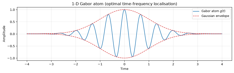
Among all signals, this one (the Gabor atom) achieves the smallest possible time-bandwidth product, $\Delta t \cdot \Delta f = 1/(4\pi)$, where $\Delta t$ and $\Delta f$ are the RMS widths of the squared (energy) envelope, the same convention used in the basics chapter. It is the most compact joint time-frequency packet that exists.

import numpy as np
import matplotlib.pyplot as plt

t = np.linspace(-4, 4, 800)
sigma, f = 1.0, 1.5
env = np.exp(-t**2 / (2 * sigma**2))
atom = env * np.cos(2 * np.pi * f * t)

fig, ax = plt.subplots(figsize=(10, 3.2))
ax.plot(t, atom, color="C0", lw=1.4, label="Gabor atom $g(t)$")
ax.plot(t, env, "--", color="C3", lw=1.2, label="Gaussian envelope")
ax.plot(t, -env, "--", color="C3", lw=1.2)
ax.set_xlabel("Time"); ax.set_ylabel("Amplitude")
ax.set_title("1-D Gabor atom (optimal time-frequency localisation)")
ax.legend(fontsize=9); ax.grid(True, alpha=0.3)
fig.tight_layout(); plt.show()

Figure 1: The 1-D Gabor atom: a Gaussian envelope times a cosine. It is the signal that meets the Gabor (uncertainty) limit with equality, the most compact time-frequency packet possible.

The step into vision is to ask the same question in two dimensions, over space instead of time. There the optimal packet is localised in position and in spatial frequency, and spatial frequency has a direction. That direction is what turns the Gabor atom into an orientation detector.

The 2-D Gabor function

A 2-D Gabor filter is a Gaussian envelope multiplying a plane wave. With the image coordinates rotated by the orientation $\theta$,

\[ x' = x\cos\theta + y\sin\theta, \qquad y' = -x\sin\theta + y\cos\theta, \]

the (complex) Gabor function is

\[ g(x, y) = \exp\!\left(-\frac{x'^2 + \gamma^2 y'^2}{2\sigma^2}\right) \exp\!\left(i\left(\tfrac{2\pi}{\lambda}\,x' + \psi\right)\right). \]

Its parameters each have a direct visual meaning:

$\theta$ is the orientation the filter is tuned to.
$\lambda$ is the wavelength of the carrier ($1/\lambda$ is the spatial frequency, the scale).
$\sigma$ sets the size of the receptive field, usually tied to $\lambda$ so that bandwidth in octaves is constant.
$\gamma$ is the aspect ratio, how elongated the field is along the edge.
$\psi$ is the phase: the real (cosine) part is an even, bar-detecting filter; the imaginary (sine) part is odd and edge-detecting.

Taking the magnitude of the complex response, $\sqrt{\text{even}^2 + \text{odd}^2}$, gives a phase-invariant measure of oriented structure: this is the standard energy model of a V1 complex cell.

from skimage.filters import gabor_kernel

fig, axes = plt.subplots(1, 4, figsize=(11, 3))
for ax, deg in zip(axes, [0, 45, 90, 135]):
    k = gabor_kernel(frequency=0.2, theta=np.deg2rad(deg), bandwidth=1.0)
    ax.imshow(k.real, cmap="gray")
    ax.set_title(f"$\\theta$ = {deg}°"); ax.set_xticks([]); ax.set_yticks([])
fig.suptitle("2-D Gabor kernels (real part)")
fig.tight_layout(); plt.show()

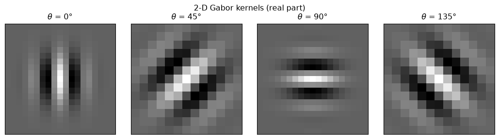
Figure 2: Real (even) parts of 2-D Gabor kernels at four orientations, same scale. Each is tuned to edges perpendicular to its stripes.

A Gabor bank tiles orientation and scale

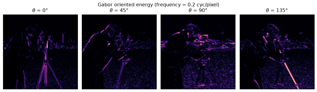
The visual cortex does not use one Gabor filter; it uses a bank spanning several orientations and several scales, so that any local edge falls into some channel. Convolving an image with the whole bank and taking magnitudes gives an oriented-energy representation: at every pixel, how much edge energy exists at each orientation and scale.

from skimage import data
from gabor import gabor_response

img = data.camera().astype(float) / 255.0
freq = 0.2
fig, axes = plt.subplots(1, 4, figsize=(11, 3.2))
for ax, deg in zip(axes, [0, 45, 90, 135]):
    resp = gabor_response(img, freq, theta=np.deg2rad(deg))
    ax.imshow(resp, cmap="magma")
    ax.set_title(f"$\\theta$ = {deg}°"); ax.set_xticks([]); ax.set_yticks([])
fig.suptitle("Gabor oriented energy (frequency = 0.2 cyc/pixel)")
fig.tight_layout(); plt.show()

Figure 3: Oriented energy of a test image at one scale. Each panel is the Gabor magnitude response for one orientation; edges perpendicular to that orientation angle (running parallel to the kernel stripes) light up.

The classic application is texture analysis: different textures excite different combinations of orientation and scale channels, so the stacked Gabor energies make a feature vector that separates materials a plain intensity histogram cannot. The same representation underlies oriented-edge maps, and the enhancement step in most fingerprint recognisers is a Gabor bank steered to the local ridge orientation. The reusable code is in gabor.py: gabor_bank builds the kernels, gabor_response gives one magnitude map, and gabor_feature_stack returns the whole oriented-energy stack.

from gabor import dominant_orientation

def grating(n=128, frequency=0.1, theta=0.0):
    y, x = np.mgrid[0:n, 0:n]
    xr = x * np.cos(theta) + y * np.sin(theta)
    return np.cos(2 * np.pi * frequency * xr)

true_deg = 30
img_g = grating(theta=np.deg2rad(true_deg), frequency=0.12)
orients = np.deg2rad(np.arange(0, 180, 15))
energies = [gabor_response(img_g, 0.12, theta=t).sum() for t in orients]
best = np.rad2deg(dominant_orientation(img_g, 0.12, orients))

fig, ax = plt.subplots(figsize=(9, 3.2))
ax.plot(np.rad2deg(orients), energies / np.max(energies), "o-")
ax.axvline(true_deg, color="C3", ls="--", label=f"true orientation ({true_deg}°)")
ax.set_xlabel("Gabor channel orientation [deg]"); ax.set_ylabel("Normalised energy")
ax.set_title(f"Dominant orientation recovered: {best:.0f}°")
ax.legend(fontsize=9); ax.grid(True, alpha=0.3)
fig.tight_layout(); plt.show()

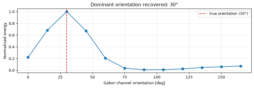
Figure 4: Recovering the orientation of a synthetic grating. The Gabor energy summed over the image peaks at the channel matching the grating’s true orientation.

The center-surround cousin: Difference of Gaussians

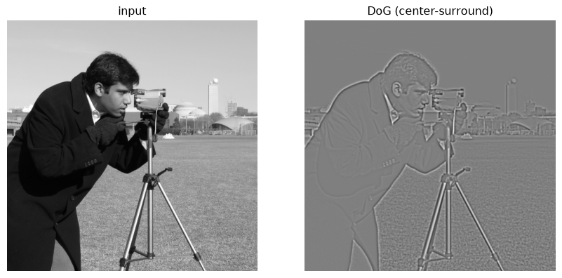
Before the cortex, the retina and the lateral geniculate nucleus use a different, simpler receptive field: a center-surround cell, excited by light in a small central spot and inhibited by light in a surrounding ring (Shapley and Enroth-Cugell 1984). This is lateral inhibition, and it sharpens edges and removes slowly varying illumination. Its standard engineering model is the Difference of Gaussians (DoG): subtract a wide Gaussian blur from a narrow one.

\[ \text{DoG}(x, y) = G_{\sigma_1}(x, y) - G_{\sigma_2}(x, y), \qquad \sigma_1 < \sigma_2. \]

Where the Gabor filter is orientation-selective, the DoG is isotropic: it responds to spots and blobs of the right size regardless of direction, which is why it is the classic blob detector and the first stage of the SIFT scale space.

from gabor import dog

d = dog(img, sigma1=1.0, sigma2=2.0)
fig, (a1, a2) = plt.subplots(1, 2, figsize=(9, 4.2))
a1.imshow(img, cmap="gray"); a1.set_title("input"); a1.axis("off")
m = np.abs(d).max()
a2.imshow(d, cmap="gray", vmin=-m, vmax=m); a2.set_title("DoG (center-surround)"); a2.axis("off")
fig.tight_layout(); plt.show()

Figure 5: Difference of Gaussians on a natural image. The center-surround response enhances edges and blobs and discards smooth gradients, mimicking retinal lateral inhibition.

Open questions and honest limits

A Gabor bank is an excellent front end for vision, but it is not a complete model of the visual cortex, and it is worth being clear about the gap.

No normalisation or nonlinearity. Real V1 neurons divide their response by the activity of their neighbours (divisive normalisation) and saturate. A linear Gabor bank has neither, so its absolute responses do not match cortical firing rates.
Fixed, not learned. The bank’s orientations and scales are chosen by hand. When receptive fields are learned from natural images (sparse coding, or the first layers of a convolutional network), Gabor-like filters emerge, but with a distribution of shapes a regular bank does not capture.
Overcomplete and non-orthogonal. Gabor filters at many orientations and scales overlap heavily; the representation is redundant, so it is good for analysis but not a tight basis for reconstruction or compression.
Separable approximation. The fast embedded implementations approximate the 2-D Gabor as separable 1-D passes, which is exact only for axis-aligned orientations; off-axis orientations carry a small approximation error. This trade-off is taken up on the embedded page.

As with the gammatone bank, these are the points where “the biology is the algorithm” turns into “the algorithm is a useful model of the biology.” Stating them is the honest version of the claim.

References

Daugman, John G. 1985. “Uncertainty Relation for Resolution in Space, Spatial Frequency, and Orientation Optimized by Two-Dimensional Visual Cortical Filters.” Journal of the Optical Society of America A 2 (7): 1160–69. https://doi.org/10.1364/JOSAA.2.001160.

Gabor, Dennis. 1946. “Theory of Communication.” Journal of the Institution of Electrical Engineers 93 (26): 429–57.

Hubel, David H., and Torsten N. Wiesel. 1962. “Receptive Fields, Binocular Interaction and Functional Architecture in the Cat’s Visual Cortex.” The Journal of Physiology 160 (1): 106–54. https://doi.org/10.1113/jphysiol.1962.sp006837.

Shapley, Robert, and Christina Enroth-Cugell. 1984. “Visual Adaptation and Retinal Gain Controls.” Progress in Retinal Research 3: 263–346.

--- title: "Gabor Filters" subtitle: "Oriented receptive fields, from the uncertainty principle to the visual cortex" --- ::: {.callout-tip title="Nature's edge detector" appearance="simple"} Hubel and Wiesel found that neurons in the primary visual cortex (V1) do not respond to light in general; each responds to an edge at a particular **orientation** and **scale**, at a particular place in the visual field [@hubel1962receptive]. The cortex tiles the image with a bank of these oriented detectors, much as the cochlea tiles sound with a bank of [gammatone channels](../gammatone-filters/index.qmd). The remarkable part, due to Daugman, is that the receptive fields look almost exactly like **Gabor functions**, the functions that are mathematically optimal at being localised in space and in spatial frequency at the same time [@daugman1985uncertainty]. ::: This page starts from a principle the [frequency-domain chapter](../../basics/05-frequency-domain.qmd#the-uncertainty-principle) already establishes, the **Gabor limit** on joint time-frequency resolution, and follows it into two dimensions, where it becomes the oriented receptive field of the visual cortex. We build a Gabor filter bank, use it for texture and orientation analysis, and meet its center-surround cousin, the Difference of Gaussians. The [embedded companion page](embedded.qmd) takes the 2-D convolution to hardware across a range of microcontrollers. ::: {.callout-note title="Prerequisites"} This topic assumes familiarity with the [frequency domain](../../basics/05-frequency-domain.qmd) and convolution. It is the 2-D, image-domain counterpart to the 1-D [gammatone filter bank](../gammatone-filters/index.qmd); reading that first is helpful but not required. ::: --- ## From the uncertainty principle to the Gabor atom The [basics chapter](../../basics/05-frequency-domain.qmd#the-uncertainty-principle) states the Gabor limit: a signal cannot be arbitrarily sharp in both time and frequency, and the product of the two spreads has a lower bound [@gabor1946theory]. A natural question is *which* signal actually reaches that bound. Gabor's answer was the **Gaussian-windowed sinusoid**: $$ g(t) = e^{-t^2 / (2\sigma^2)} \cos(2\pi f t + \psi). $$ Among all signals, this one (the **Gabor atom**) achieves the smallest possible time-bandwidth product, $\Delta t \cdot \Delta f = 1/(4\pi)$, where $\Delta t$ and $\Delta f$ are the RMS widths of the squared (energy) envelope, the same convention used in the [basics chapter](../../basics/05-frequency-domain.qmd#the-uncertainty-principle). It is the most compact joint time-frequency packet that exists. ```{python} #| label: fig-1d-atom #| fig-cap: "The 1-D Gabor atom: a Gaussian envelope times a cosine. It is the signal that meets the Gabor (uncertainty) limit with equality, the most compact time-frequency packet possible." import numpy as np import matplotlib.pyplot as plt t = np.linspace(-4, 4, 800) sigma, f = 1.0, 1.5 env = np.exp(-t**2 / (2 * sigma**2)) atom = env * np.cos(2 * np.pi * f * t) fig, ax = plt.subplots(figsize=(10, 3.2)) ax.plot(t, atom, color="C0", lw=1.4, label="Gabor atom $g(t)$") ax.plot(t, env, "--", color="C3", lw=1.2, label="Gaussian envelope") ax.plot(t, -env, "--", color="C3", lw=1.2) ax.set_xlabel("Time"); ax.set_ylabel("Amplitude") ax.set_title("1-D Gabor atom (optimal time-frequency localisation)") ax.legend(fontsize=9); ax.grid(True, alpha=0.3) fig.tight_layout(); plt.show() ``` The step into vision is to ask the same question in two dimensions, over space instead of time. There the optimal packet is localised in **position** and in **spatial frequency**, and spatial frequency has a direction. That direction is what turns the Gabor atom into an orientation detector. --- ## The 2-D Gabor function A 2-D Gabor filter is a Gaussian envelope multiplying a plane wave. With the image coordinates rotated by the orientation $\theta$, $$ x' = x\cos\theta + y\sin\theta, \qquad y' = -x\sin\theta + y\cos\theta, $$ the (complex) Gabor function is $$ g(x, y) = \exp\!\left(-\frac{x'^2 + \gamma^2 y'^2}{2\sigma^2}\right) \exp\!\left(i\left(\tfrac{2\pi}{\lambda}\,x' + \psi\right)\right). $$ Its parameters each have a direct visual meaning: - $\theta$ is the **orientation** the filter is tuned to. - $\lambda$ is the **wavelength** of the carrier ($1/\lambda$ is the spatial frequency, the scale). - $\sigma$ sets the **size** of the receptive field, usually tied to $\lambda$ so that bandwidth in octaves is constant. - $\gamma$ is the **aspect ratio**, how elongated the field is along the edge. - $\psi$ is the **phase**: the real (cosine) part is an even, bar-detecting filter; the imaginary (sine) part is odd and edge-detecting. Taking the magnitude of the complex response, $\sqrt{\text{even}^2 + \text{odd}^2}$, gives a **phase-invariant** measure of oriented structure: this is the standard energy model of a V1 complex cell. ```{python} #| label: fig-2d-kernels #| fig-cap: "Real (even) parts of 2-D Gabor kernels at four orientations, same scale. Each is tuned to edges perpendicular to its stripes." from skimage.filters import gabor_kernel fig, axes = plt.subplots(1, 4, figsize=(11, 3)) for ax, deg in zip(axes, [0, 45, 90, 135]): k = gabor_kernel(frequency=0.2, theta=np.deg2rad(deg), bandwidth=1.0) ax.imshow(k.real, cmap="gray") ax.set_title(f"$\\theta$ = {deg}°"); ax.set_xticks([]); ax.set_yticks([]) fig.suptitle("2-D Gabor kernels (real part)") fig.tight_layout(); plt.show() ``` --- ## A Gabor bank tiles orientation and scale The visual cortex does not use one Gabor filter; it uses a **bank** spanning several orientations and several scales, so that any local edge falls into some channel. Convolving an image with the whole bank and taking magnitudes gives an *oriented-energy* representation: at every pixel, how much edge energy exists at each orientation and scale. ```{python} #| label: fig-oriented-energy #| fig-cap: "Oriented energy of a test image at one scale. Each panel is the Gabor magnitude response for one orientation; edges perpendicular to that orientation angle (running parallel to the kernel stripes) light up." from skimage import data from gabor import gabor_response img = data.camera().astype(float) / 255.0 freq = 0.2 fig, axes = plt.subplots(1, 4, figsize=(11, 3.2)) for ax, deg in zip(axes, [0, 45, 90, 135]): resp = gabor_response(img, freq, theta=np.deg2rad(deg)) ax.imshow(resp, cmap="magma") ax.set_title(f"$\\theta$ = {deg}°"); ax.set_xticks([]); ax.set_yticks([]) fig.suptitle("Gabor oriented energy (frequency = 0.2 cyc/pixel)") fig.tight_layout(); plt.show() ``` The classic application is **texture analysis**: different textures excite different combinations of orientation and scale channels, so the stacked Gabor energies make a feature vector that separates materials a plain intensity histogram cannot. The same representation underlies oriented-edge maps, and the enhancement step in most fingerprint recognisers is a Gabor bank steered to the local ridge orientation. The reusable code is in [`gabor.py`](gabor.py): `gabor_bank` builds the kernels, `gabor_response` gives one magnitude map, and `gabor_feature_stack` returns the whole oriented-energy stack. ```{python} #| label: fig-dominant #| fig-cap: "Recovering the orientation of a synthetic grating. The Gabor energy summed over the image peaks at the channel matching the grating's true orientation." from gabor import dominant_orientation def grating(n=128, frequency=0.1, theta=0.0): y, x = np.mgrid[0:n, 0:n] xr = x * np.cos(theta) + y * np.sin(theta) return np.cos(2 * np.pi * frequency * xr) true_deg = 30 img_g = grating(theta=np.deg2rad(true_deg), frequency=0.12) orients = np.deg2rad(np.arange(0, 180, 15)) energies = [gabor_response(img_g, 0.12, theta=t).sum() for t in orients] best = np.rad2deg(dominant_orientation(img_g, 0.12, orients)) fig, ax = plt.subplots(figsize=(9, 3.2)) ax.plot(np.rad2deg(orients), energies / np.max(energies), "o-") ax.axvline(true_deg, color="C3", ls="--", label=f"true orientation ({true_deg}°)") ax.set_xlabel("Gabor channel orientation [deg]"); ax.set_ylabel("Normalised energy") ax.set_title(f"Dominant orientation recovered: {best:.0f}°") ax.legend(fontsize=9); ax.grid(True, alpha=0.3) fig.tight_layout(); plt.show() ``` --- ## The center-surround cousin: Difference of Gaussians Before the cortex, the retina and the lateral geniculate nucleus use a different, simpler receptive field: a **center-surround** cell, excited by light in a small central spot and inhibited by light in a surrounding ring [@shapley1984visual]. This is **lateral inhibition**, and it sharpens edges and removes slowly varying illumination. Its standard engineering model is the **Difference of Gaussians** (DoG): subtract a wide Gaussian blur from a narrow one. $$ \text{DoG}(x, y) = G_{\sigma_1}(x, y) - G_{\sigma_2}(x, y), \qquad \sigma_1 < \sigma_2. $$ Where the Gabor filter is orientation-selective, the DoG is isotropic: it responds to spots and blobs of the right size regardless of direction, which is why it is the classic **blob detector** and the first stage of the SIFT scale space. ```{python} #| label: fig-dog #| fig-cap: "Difference of Gaussians on a natural image. The center-surround response enhances edges and blobs and discards smooth gradients, mimicking retinal lateral inhibition." from gabor import dog d = dog(img, sigma1=1.0, sigma2=2.0) fig, (a1, a2) = plt.subplots(1, 2, figsize=(9, 4.2)) a1.imshow(img, cmap="gray"); a1.set_title("input"); a1.axis("off") m = np.abs(d).max() a2.imshow(d, cmap="gray", vmin=-m, vmax=m); a2.set_title("DoG (center-surround)"); a2.axis("off") fig.tight_layout(); plt.show() ``` --- ## Open questions and honest limits A Gabor bank is an excellent **front end** for vision, but it is not a complete model of the visual cortex, and it is worth being clear about the gap. - **No normalisation or nonlinearity.** Real V1 neurons divide their response by the activity of their neighbours (divisive normalisation) and saturate. A linear Gabor bank has neither, so its absolute responses do not match cortical firing rates. - **Fixed, not learned.** The bank's orientations and scales are chosen by hand. When receptive fields are *learned* from natural images (sparse coding, or the first layers of a convolutional network), Gabor-like filters emerge, but with a distribution of shapes a regular bank does not capture. - **Overcomplete and non-orthogonal.** Gabor filters at many orientations and scales overlap heavily; the representation is redundant, so it is good for analysis but not a tight basis for reconstruction or compression. - **Separable approximation.** The fast embedded implementations approximate the 2-D Gabor as separable 1-D passes, which is exact only for axis-aligned orientations; off-axis orientations carry a small approximation error. This trade-off is taken up on the [embedded page](embedded.qmd). As with the gammatone bank, these are the points where "the biology is the algorithm" turns into "the algorithm is a useful model of the biology." Stating them is the honest version of the claim. --- ## References ::: {#refs} :::