Modelling the cochlea as a bank of bandpass filters
Nature’s filter bank
The basilar membrane inside the cochlea is a frequency analyser. It is stiff and narrow at one end, floppy and wide at the other, so each point along its length resonates at its own characteristic frequency, high frequencies near the base and low frequencies near the apex (Robles and Ruggero 2001). A sound entering the ear is spread out into a continuous map of frequency versus place, and the auditory nerve reads off that map. The gammatone filter bank is the standard digital model of exactly this behaviour: one bandpass filter per place, with bandwidths that match the measured tuning of auditory nerve fibres.
This page builds a gammatone filter bank from first principles, lays its channels out on the auditory (ERB) frequency scale, and shows that each channel is nothing more than a cascade of four biquad sections. That last point is what makes the algorithm practical on a microcontroller, which is taken up in the embedded companion page.
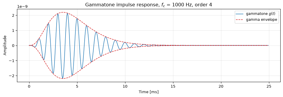
If you tap a single point on the basilar membrane with a click, it rings: it oscillates at its characteristic frequency while the amplitude rises and then decays. Patterson and colleagues found that the impulse response of an auditory filter is captured very well by a gamma-distribution envelope multiplying a tone(Patterson et al. 1992). The name gammatone is the contraction of those two words.
The impulse response is
\[
g(t) = a\, t^{\,n-1} e^{-2\pi b t} \cos(2\pi f_c t + \phi), \qquad t \ge 0,
\]
with four interpretable parameters:
\(f_c\) is the centre frequency: the carrier the filter is tuned to.
\(n\) is the order: the power on \(t\) shapes the envelope. The auditory data are fit well by \(n = 4\), which is the value used almost universally.
\(b\) is the bandwidth parameter: how fast the envelope decays, and therefore how sharply the filter is tuned.
\(a\) and \(\phi\) are an amplitude and a starting phase, which we normally fix by convention.
import numpy as npimport matplotlib.pyplot as pltfs =16000fc =1000.0n =4# Bandwidth parameter for a 4th-order gammatone: b = 1.019 * ERB(fc)erb =24.7* (0.00437* fc +1.0)b =1.019* erbt = np.arange(0, 0.025, 1/ fs)envelope = t ** (n -1) * np.exp(-2* np.pi * b * t)g = envelope * np.cos(2* np.pi * fc * t)envelope_norm = envelope / envelope.max() * np.abs(g).max()fig, ax = plt.subplots(figsize=(10, 3.5))ax.plot(t *1e3, g, color="C0", lw=1.2, label="gammatone $g(t)$")ax.plot(t *1e3, envelope_norm, "--", color="C3", lw=1.2, label="gamma envelope")ax.plot(t *1e3, -envelope_norm, "--", color="C3", lw=1.2)ax.set_xlabel("Time [ms]")ax.set_ylabel("Amplitude")ax.set_title(f"Gammatone impulse response, $f_c$ = {fc:.0f} Hz, order {n}")ax.legend(fontsize=9)ax.grid(True, alpha=0.3)fig.tight_layout()plt.show()
Figure 1: Gammatone impulse response at 1 kHz (order 4). The gamma envelope (dashed) rises then decays; the carrier oscillates at the centre frequency inside it.
The envelope is the “gamma” part (it has the shape of a gamma probability density), and the cosine is the “tone” part. Higher \(f_c\) means more oscillations packed under the same envelope; larger \(b\) means a faster decay and a wider passband.
The ERB scale: how wide is each filter?
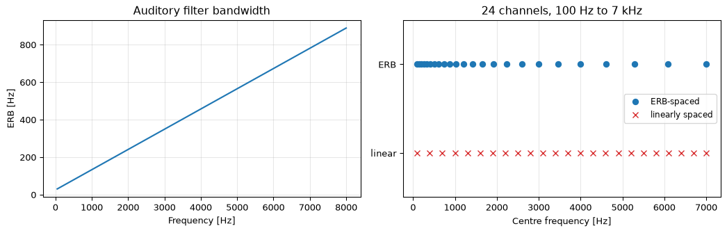
A filter bank needs two design choices: where to put the centre frequencies, and how wide to make each filter. The cochlea answers both with a single idea. Auditory filters are narrow at low frequencies and progressively wider at high frequencies, and the natural unit for this is the equivalent rectangular bandwidth (ERB): the width of the ideal rectangular filter that would pass the same total power as the real, rounded auditory filter.
\[
\mathrm{ERB}(f) = 24.7\,\bigl(0.00437\, f + 1\bigr) \quad \text{[Hz]},
\]
with \(f\) in Hz. At 1 kHz this gives about 133 Hz; at 4 kHz it has grown to about 457 Hz. The bandwidth parameter of the gammatone is tied to this by \(b = 1.019\,\mathrm{ERB}(f_c)\) for the 4th-order filter (Slaney 1993).
To place the channels, we integrate that bandwidth into the ERB-rate scale, which counts how many ERBs fit below a given frequency:
\[
E(f) = 21.4\,\log_{10}\bigl(0.00437\, f + 1\bigr).
\]
Spacing centre frequencies equally on \(E\) puts them densely where the ear has fine resolution and sparsely where it does not, mirroring the even spacing of hair cells along the membrane.
Figure 2: Left: ERB grows roughly linearly with frequency. Right: 24 channels spaced equally on the ERB-rate scale cluster at low frequencies and spread out at high frequencies, unlike linearly spaced bins.
A gammatone channel is a cascade of biquads
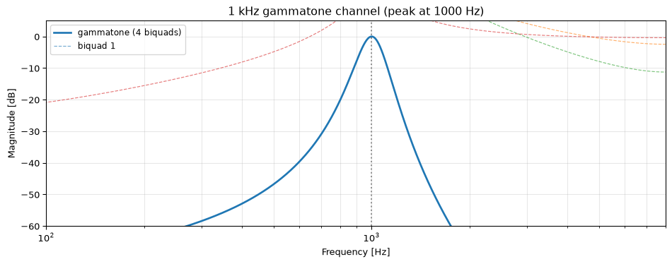
We could realise the filter by sampling \(g(t)\) directly into a long FIR, but that is wasteful: a low-frequency channel rings for tens of milliseconds, which is hundreds of taps. The efficient route, due to Slaney, approximates the gammatone with an IIR filter instead (Slaney 1993). For the standard 4th-order gammatone this is an 8th-order transfer function, and any transfer function of even order factors into second-order sections. In other words:
A 4th-order gammatone channel is exactly a cascade of four biquads, with resonant poles clustered tightly at \(f_c\) and different numerator zeros in each section.
This is the same second-order section that the biquad topic builds filters from, which is why an auditory filter bank costs so little to run. SciPy designs Slaney’s filter directly; we just factor it into sections with tf2sos.
Figure 3: Magnitude response of the 1 kHz gammatone channel and the four biquad sections it factors into. The cascade peaks at the centre frequency with the rounded, asymmetric skirts characteristic of auditory tuning.
The reusable implementation lives in gammatone.py: erb_space lays out the centre frequencies, gammatone_sos returns the four-section cascade for one channel, and gammatone_filterbank runs a whole bank with sosfilt.
The whole bank: a cochleagram
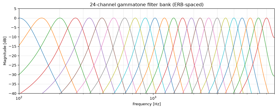
Stacking the channels gives the filter bank. Its set of overlapping magnitude responses tiles the frequency axis the way the basilar membrane tiles its length.
from gammatone import erb_space as erb_space_mod, make_filterbankcfs = erb_space_mod(100, 7000, 24)bank = make_filterbank(fs, cfs)fig, ax = plt.subplots(figsize=(10, 4))for sos_ch in bank: w, H = signal.sosfreqz(sos_ch, worN=4096, fs=fs) ax.semilogx(w[1:], 20* np.log10(np.maximum(np.abs(H[1:]), 1e-6)), lw=1)ax.set_xlabel("Frequency [Hz]")ax.set_ylabel("Magnitude [dB]")ax.set_ylim(-40, 5)ax.set_xlim(100, fs /2)ax.set_title("24-channel gammatone filter bank (ERB-spaced)")ax.grid(True, alpha=0.3, which="both")fig.tight_layout()plt.show()
Figure 4: A 24-channel gammatone filter bank, 100 Hz to 7 kHz. The filters overlap and widen toward high frequencies, exactly as ERB spacing dictates.
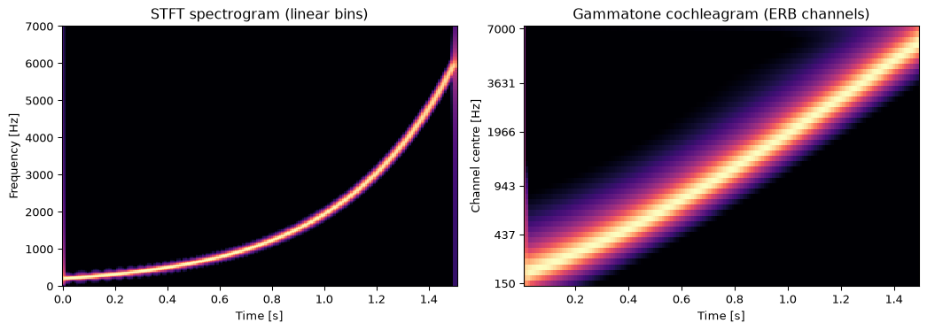
Running a sound through the bank and measuring the energy in each channel over time produces a cochleagram: the auditory counterpart of a spectrogram. The difference is the frequency axis. A spectrogram has linearly spaced bins from a fixed-length DFT; a cochleagram has ERB-spaced channels, so it spends its resolution where hearing does, packing detail into the low frequencies that carry speech formants and pitch.
from gammatone import cochleagram# A logarithmic chirp from 200 Hz to 6 kHzdur =1.5t = np.arange(0, dur, 1/ fs)x = signal.chirp(t, f0=200, t1=dur, f1=6000, method="logarithmic")cfs_demo = erb_space_mod(150, 7000, 48)coch, times = cochleagram(x, fs, cfs_demo, frame_ms=20, hop_ms=8)f_stft, t_stft, Z = signal.stft(x, fs=fs, nperseg=512, noverlap=384)S_db =20* np.log10(np.maximum(np.abs(Z) / np.abs(Z).max(), 1e-4))fig, (ax1, ax2) = plt.subplots(1, 2, figsize=(11, 4), sharey=False)ax1.pcolormesh(t_stft, f_stft, S_db, shading="auto", vmin=-60, vmax=0, cmap="magma")ax1.set_title("STFT spectrogram (linear bins)")ax1.set_xlabel("Time [s]")ax1.set_ylabel("Frequency [Hz]")ax1.set_ylim(0, 7000)ax2.pcolormesh(times, np.arange(len(cfs_demo)), coch, shading="auto", vmin=-60, vmax=0, cmap="magma")yt = np.linspace(0, len(cfs_demo) -1, 6).astype(int)ax2.set_yticks(yt, [f"{cfs_demo[i]:.0f}"for i in yt])ax2.set_title("Gammatone cochleagram (ERB channels)")ax2.set_xlabel("Time [s]")ax2.set_ylabel("Channel centre [Hz]")fig.tight_layout()plt.show()
Figure 5: A rising chirp seen by an STFT spectrogram (left) and a gammatone cochleagram (right). The cochleagram stretches the low frequencies and compresses the highs, matching auditory resolution.
This auditory front end is the first stage of many speech and audio systems: it feeds computational auditory scene analysis, robust speech recognisers, and hearing-aid processors (Rosenthal and Okuno 1998). The same cochleagram is also where mel- and gammatone-cepstral features begin, which is why the auditory filter bank shows up again the moment we start extracting features for machine listening.
Open questions and honest limits
The gammatone bank is a good model of the passive, linear cochlea, but the real cochlea is neither.
No active gain. The living cochlea has an active feedback mechanism (the outer hair cells) that sharpens tuning and boosts faint sounds by up to 40 dB. The gammatone is a fixed linear filter and captures none of this. Models that add level-dependent gain, such as the dual-resonance nonlinear (DRNL) and the cascade-of-asymmetric-resonators (CARFAC) families, exist but are considerably more involved.
Level-independent bandwidth. Because the gammatone is linear, its bandwidth does not change with input level. Real auditory filters broaden as sounds get louder. For analysis at a single moderate level this rarely matters, but it does for wide-dynamic-range audio.
No two-tone suppression. A loud tone in one channel can suppress the response to a second tone in the cochlea. A bank of independent linear filters cannot reproduce this, since the channels never interact.
Phase convention. The starting phase \(\phi\) and whether the filter is run causally or zero-phase affects fine timing across channels. For energy-based features (the cochleagram above) this washes out; for models that rely on cross-channel timing, it has to be handled with care.
None of these undermine the gammatone as a front end. They mark where “the biology is the algorithm” stops being literally true and the model becomes an approximation, which is exactly the kind of boundary worth stating plainly.
References
Glasberg, Brian R., and Brian C. J. Moore. 1990. “Derivation of Auditory Filter Shapes from Notched-Noise Data.”Hearing Research 47 (1-2): 103–38. https://doi.org/10.1016/0378-5955(90)90170-T.
Patterson, Roy D., K. Robinson, John Holdsworth, D. McKeown, C. Zhang, and M. Allerhand. 1992. “Complex Sounds and Auditory Images.” In Auditory Physiology and Perception, 83:429–46. Advances in the Biosciences. Pergamon. https://doi.org/10.1016/B978-0-08-041847-6.50054-X.
Robles, Luis, and Mario A. Ruggero. 2001. “Mechanics of the Mammalian Cochlea.”Physiological Reviews 81 (3): 1305–52.
Rosenthal, David F., and Hiroshi G. Okuno. 1998. Computational Auditory Scene Analysis. Lawrence Erlbaum Associates.
Slaney, Malcolm. 1993. “An Efficient Implementation of the Patterson-Holdsworth Auditory Filter Bank.” 35. Apple Computer, Perception Group.
Source Code
---title: "Gammatone Filters"subtitle: "Modelling the cochlea as a bank of bandpass filters"---::: {.callout-tip title="Nature's filter bank" appearance="simple"}The basilar membrane inside the cochlea is a frequency analyser. It is stiff and narrow at one end, floppy and wide at the other, so each point along its length resonates at its own characteristic frequency, high frequencies near the base and low frequencies near the apex [@robles2001mechanics]. A sound entering the ear is spread out into a continuous map of frequency versus place, and the auditory nerve reads off that map. The gammatone filter bank is the standard digital model of exactly this behaviour: one bandpass filter per place, with bandwidths that match the measured tuning of auditory nerve fibres.:::This page builds a gammatone filter bank from first principles, lays its channels out on the auditory (ERB) frequency scale, and shows that each channel is nothing more than a cascade of four [biquad sections](../biquad/index.qmd). That last point is what makes the algorithm practical on a microcontroller, which is taken up in the [embedded companion page](embedded.qmd).::: {.callout-note title="Prerequisites"}This topic assumes familiarity with the [frequency domain](../../basics/05-frequency-domain.qmd), [IIR filter design](../../basics/06-filter-design.qmd), and [biquad filters](../biquad/index.qmd). The cochlea was introduced as a filter bank in the [pitch detection](../pitch-detection/index.qmd) topic; here we make that filter bank explicit.:::---## From basilar membrane to impulse responseIf you tap a single point on the basilar membrane with a click, it rings: it oscillates at its characteristic frequency while the amplitude rises and then decays. Patterson and colleagues found that the impulse response of an auditory filter is captured very well by a **gamma**-distribution envelope multiplying a **tone** [@patterson1992complex]. The name *gammatone* is the contraction of those two words.The impulse response is$$g(t) = a\, t^{\,n-1} e^{-2\pi b t} \cos(2\pi f_c t + \phi), \qquad t \ge 0,$$with four interpretable parameters:- $f_c$ is the **centre frequency**: the carrier the filter is tuned to.- $n$ is the **order**: the power on $t$ shapes the envelope. The auditory data are fit well by $n = 4$, which is the value used almost universally.- $b$ is the **bandwidth** parameter: how fast the envelope decays, and therefore how sharply the filter is tuned.- $a$ and $\phi$ are an amplitude and a starting phase, which we normally fix by convention.```{python}#| label: fig-impulse#| fig-cap: "Gammatone impulse response at 1 kHz (order 4). The gamma envelope (dashed) rises then decays; the carrier oscillates at the centre frequency inside it."import numpy as npimport matplotlib.pyplot as pltfs =16000fc =1000.0n =4# Bandwidth parameter for a 4th-order gammatone: b = 1.019 * ERB(fc)erb =24.7* (0.00437* fc +1.0)b =1.019* erbt = np.arange(0, 0.025, 1/ fs)envelope = t ** (n -1) * np.exp(-2* np.pi * b * t)g = envelope * np.cos(2* np.pi * fc * t)envelope_norm = envelope / envelope.max() * np.abs(g).max()fig, ax = plt.subplots(figsize=(10, 3.5))ax.plot(t *1e3, g, color="C0", lw=1.2, label="gammatone $g(t)$")ax.plot(t *1e3, envelope_norm, "--", color="C3", lw=1.2, label="gamma envelope")ax.plot(t *1e3, -envelope_norm, "--", color="C3", lw=1.2)ax.set_xlabel("Time [ms]")ax.set_ylabel("Amplitude")ax.set_title(f"Gammatone impulse response, $f_c$ = {fc:.0f} Hz, order {n}")ax.legend(fontsize=9)ax.grid(True, alpha=0.3)fig.tight_layout()plt.show()```The envelope is the "gamma" part (it has the shape of a gamma probability density), and the cosine is the "tone" part. Higher $f_c$ means more oscillations packed under the same envelope; larger $b$ means a faster decay and a wider passband.---## The ERB scale: how wide is each filter?A filter bank needs two design choices: where to put the centre frequencies, and how wide to make each filter. The cochlea answers both with a single idea. Auditory filters are **narrow at low frequencies and progressively wider at high frequencies**, and the natural unit for this is the **equivalent rectangular bandwidth** (ERB): the width of the ideal rectangular filter that would pass the same total power as the real, rounded auditory filter.Glasberg and Moore fit the measured human ERB with a simple line [@glasbergmoore1990]:$$\mathrm{ERB}(f) = 24.7\,\bigl(0.00437\, f + 1\bigr) \quad \text{[Hz]},$$with $f$ in Hz. At 1 kHz this gives about 133 Hz; at 4 kHz it has grown to about 457 Hz. The bandwidth parameter of the gammatone is tied to this by $b = 1.019\,\mathrm{ERB}(f_c)$ for the 4th-order filter [@slaney1993efficient].To place the channels, we integrate that bandwidth into the **ERB-rate scale**, which counts how many ERBs fit below a given frequency:$$E(f) = 21.4\,\log_{10}\bigl(0.00437\, f + 1\bigr).$$Spacing centre frequencies *equally on $E$* puts them densely where the ear has fine resolution and sparsely where it does not, mirroring the even spacing of hair cells along the membrane.```{python}#| label: fig-erb-spacing#| fig-cap: "Left: ERB grows roughly linearly with frequency. Right: 24 channels spaced equally on the ERB-rate scale cluster at low frequencies and spread out at high frequencies, unlike linearly spaced bins."def erb_of(f):return24.7* (0.00437* np.asarray(f, float) +1.0)def hz_to_erb_rate(f):return21.4* np.log10(0.00437* np.asarray(f, float) +1.0)def erb_rate_to_hz(e):return (10** (np.asarray(e, float) /21.4) -1.0) /0.00437def erb_space(low, high, n_ch): e = np.linspace(hz_to_erb_rate(low), hz_to_erb_rate(high), n_ch)return erb_rate_to_hz(e)f = np.linspace(50, 8000, 400)cfs = erb_space(100, 7000, 24)lin = np.linspace(100, 7000, 24)fig, (ax1, ax2) = plt.subplots(1, 2, figsize=(11, 3.6))ax1.plot(f, erb_of(f), color="C0", lw=1.6)ax1.set_xlabel("Frequency [Hz]")ax1.set_ylabel("ERB [Hz]")ax1.set_title("Auditory filter bandwidth")ax1.grid(True, alpha=0.3)ax2.plot(cfs, np.ones_like(cfs), "o", color="C0", label="ERB-spaced")ax2.plot(lin, np.zeros_like(lin), "x", color="C3", label="linearly spaced")ax2.set_xlabel("Centre frequency [Hz]")ax2.set_yticks([0, 1], ["linear", "ERB"])ax2.set_ylim(-0.5, 1.5)ax2.set_title("24 channels, 100 Hz to 7 kHz")ax2.legend(fontsize=9, loc="center right")ax2.grid(True, alpha=0.3, axis="x")fig.tight_layout()plt.show()```---## A gammatone channel is a cascade of biquadsWe could realise the filter by sampling $g(t)$ directly into a long FIR, but that is wasteful: a low-frequency channel rings for tens of milliseconds, which is hundreds of taps. The efficient route, due to Slaney, approximates the gammatone with an **IIR filter** instead [@slaney1993efficient]. For the standard 4th-order gammatone this is an 8th-order transfer function, and any transfer function of even order factors into second-order sections. In other words:> A 4th-order gammatone channel is exactly a cascade of **four biquads**, with resonant poles clustered tightly at $f_c$ and different numerator zeros in each section.This is the same second-order section that the [biquad topic](../biquad/index.qmd) builds filters from, which is why an auditory filter bank costs so little to run. SciPy designs Slaney's filter directly; we just factor it into sections with `tf2sos`.```{python}import numpy as npfrom scipy import signalfs =16000fc =1000.0b_coef, a_coef = signal.gammatone(fc, ftype="iir", fs=fs)sos = signal.tf2sos(b_coef, a_coef)print(f"Transfer function: {len(b_coef)} numerator, {len(a_coef)} denominator coefficients")print(f"Factored into {sos.shape[0]} biquad sections (one cascade = one channel)")``````{python}#| label: fig-channel-response#| fig-cap: "Magnitude response of the 1 kHz gammatone channel and the four biquad sections it factors into. The cascade peaks at the centre frequency with the rounded, asymmetric skirts characteristic of auditory tuning."w, H = signal.sosfreqz(sos, worN=8192, fs=fs)peak_hz = w[np.argmax(np.abs(H))]fig, ax = plt.subplots(figsize=(10, 4))ax.semilogx(w[1:], 20* np.log10(np.maximum(np.abs(H[1:]), 1e-6)), color="C0", lw=2, label="gammatone (4 biquads)")for k, section inenumerate(sos): wk, Hk = signal.sosfreqz(section.reshape(1, 6), worN=8192, fs=fs) ax.semilogx(wk[1:], 20* np.log10(np.maximum(np.abs(Hk[1:]), 1e-6)),"--", lw=0.9, alpha=0.6, label=f"biquad {k +1}"if k ==0elseNone)ax.axvline(fc, color="k", ls=":", alpha=0.4)ax.set_xlabel("Frequency [Hz]")ax.set_ylabel("Magnitude [dB]")ax.set_ylim(-60, 5)ax.set_xlim(100, fs /2)ax.set_title(f"1 kHz gammatone channel (peak at {peak_hz:.0f} Hz)")ax.legend(fontsize=9)ax.grid(True, alpha=0.3, which="both")fig.tight_layout()plt.show()```The reusable implementation lives in [`gammatone.py`](gammatone.py): `erb_space` lays out the centre frequencies, `gammatone_sos` returns the four-section cascade for one channel, and `gammatone_filterbank` runs a whole bank with `sosfilt`.---## The whole bank: a cochleagramStacking the channels gives the filter bank. Its set of overlapping magnitude responses tiles the frequency axis the way the basilar membrane tiles its length.```{python}#| label: fig-bank#| fig-cap: "A 24-channel gammatone filter bank, 100 Hz to 7 kHz. The filters overlap and widen toward high frequencies, exactly as ERB spacing dictates."from gammatone import erb_space as erb_space_mod, make_filterbankcfs = erb_space_mod(100, 7000, 24)bank = make_filterbank(fs, cfs)fig, ax = plt.subplots(figsize=(10, 4))for sos_ch in bank: w, H = signal.sosfreqz(sos_ch, worN=4096, fs=fs) ax.semilogx(w[1:], 20* np.log10(np.maximum(np.abs(H[1:]), 1e-6)), lw=1)ax.set_xlabel("Frequency [Hz]")ax.set_ylabel("Magnitude [dB]")ax.set_ylim(-40, 5)ax.set_xlim(100, fs /2)ax.set_title("24-channel gammatone filter bank (ERB-spaced)")ax.grid(True, alpha=0.3, which="both")fig.tight_layout()plt.show()```Running a sound through the bank and measuring the energy in each channel over time produces a **cochleagram**: the auditory counterpart of a spectrogram. The difference is the frequency axis. A spectrogram has linearly spaced bins from a fixed-length DFT; a cochleagram has ERB-spaced channels, so it spends its resolution where hearing does, packing detail into the low frequencies that carry speech formants and pitch.```{python}#| label: fig-cochleagram#| fig-cap: "A rising chirp seen by an STFT spectrogram (left) and a gammatone cochleagram (right). The cochleagram stretches the low frequencies and compresses the highs, matching auditory resolution."from gammatone import cochleagram# A logarithmic chirp from 200 Hz to 6 kHzdur =1.5t = np.arange(0, dur, 1/ fs)x = signal.chirp(t, f0=200, t1=dur, f1=6000, method="logarithmic")cfs_demo = erb_space_mod(150, 7000, 48)coch, times = cochleagram(x, fs, cfs_demo, frame_ms=20, hop_ms=8)f_stft, t_stft, Z = signal.stft(x, fs=fs, nperseg=512, noverlap=384)S_db =20* np.log10(np.maximum(np.abs(Z) / np.abs(Z).max(), 1e-4))fig, (ax1, ax2) = plt.subplots(1, 2, figsize=(11, 4), sharey=False)ax1.pcolormesh(t_stft, f_stft, S_db, shading="auto", vmin=-60, vmax=0, cmap="magma")ax1.set_title("STFT spectrogram (linear bins)")ax1.set_xlabel("Time [s]")ax1.set_ylabel("Frequency [Hz]")ax1.set_ylim(0, 7000)ax2.pcolormesh(times, np.arange(len(cfs_demo)), coch, shading="auto", vmin=-60, vmax=0, cmap="magma")yt = np.linspace(0, len(cfs_demo) -1, 6).astype(int)ax2.set_yticks(yt, [f"{cfs_demo[i]:.0f}"for i in yt])ax2.set_title("Gammatone cochleagram (ERB channels)")ax2.set_xlabel("Time [s]")ax2.set_ylabel("Channel centre [Hz]")fig.tight_layout()plt.show()```This auditory front end is the first stage of many speech and audio systems: it feeds computational auditory scene analysis, robust speech recognisers, and hearing-aid processors [@rosenthal1998computational]. The same cochleagram is also where mel- and gammatone-cepstral features begin, which is why the auditory filter bank shows up again the moment we start extracting features for machine listening.---## Open questions and honest limitsThe gammatone bank is a good model of the **passive, linear** cochlea, but the real cochlea is neither.- **No active gain.** The living cochlea has an active feedback mechanism (the outer hair cells) that sharpens tuning and boosts faint sounds by up to 40 dB. The gammatone is a fixed linear filter and captures none of this. Models that add level-dependent gain, such as the dual-resonance nonlinear (DRNL) and the cascade-of-asymmetric-resonators (CARFAC) families, exist but are considerably more involved.- **Level-independent bandwidth.** Because the gammatone is linear, its bandwidth does not change with input level. Real auditory filters broaden as sounds get louder. For analysis at a single moderate level this rarely matters, but it does for wide-dynamic-range audio.- **No two-tone suppression.** A loud tone in one channel can suppress the response to a second tone in the cochlea. A bank of independent linear filters cannot reproduce this, since the channels never interact.- **Phase convention.** The starting phase $\phi$ and whether the filter is run causally or zero-phase affects fine timing across channels. For energy-based features (the cochleagram above) this washes out; for models that rely on cross-channel timing, it has to be handled with care.None of these undermine the gammatone as a front end. They mark where "the biology is the algorithm" stops being literally true and the model becomes an approximation, which is exactly the kind of boundary worth stating plainly.---## References::: {#refs}:::