Mel-Frequency Cepstral Coefficients

Turning a spectrum into a short, decorrelated fingerprint of a sound

Ask a spectrogram what a vowel sounds like and it hands you hundreds of numbers per frame, most of them redundant. Ask an MFCC front end the same question and it hands you thirteen. Those thirteen numbers describe the shape of the spectral envelope, warped to match how human hearing resolves frequency and decorrelated so a simple classifier can use them directly. This compression is why the MFCC was the feature behind a generation of speech recognisers (Davis and Mermelstein 1980; Rabiner and Juang 1993), and why it still anchors small keyword spotters that have to run on a coin cell.

This page is the practitioner’s walk through the pipeline. It is a fixed sequence of small, cheap steps, and the interesting part is what each one is for and what it throws away. We build it on top of the two topics before it: the STFT supplies the framing and the per-frame spectrum, and the spectral features page is the sibling that summarises that spectrum a different way. MFCC is the speech-flavoured cousin.

Prerequisites

This builds on the STFT (framing, windowing, the per-frame spectrum) and reads naturally after spectral features. The clean, importable code is in mfcc.py, checked by test_mfcc.py. The embedded companion, a wakeword detector on the metal, turns this front end into a working classifier.

The pipeline at a glance

An MFCC vector is built by passing each short frame of audio through a fixed chain:

Pre-emphasis: a one-tap high-pass that boosts the weak high frequencies of voiced speech.
Framing and windowing: cut into ~25 ms frames at a ~10 ms hop, taper each one. This is exactly the STFT front end.
Power spectrum: the periodogram of each frame.
Mel filterbank: sum that power into a couple of dozen perceptually-spaced bands.
Log: take the logarithm of each band energy.
DCT: a discrete cosine transform that decorrelates the log-band energies; keep the low-order coefficients.
Deltas (optional): append first and second time differences to capture how the coefficients move.

The first half (steps 1 to 5) is the cepstral idea borrowed from speech analysis: separate the slowly-varying vocal-tract envelope from the fast pitch detail. The DCT in step 6 is the twist that makes the result compact and uncorrelated. We take the steps in order.

Pre-emphasis: tilting the spectrum back up

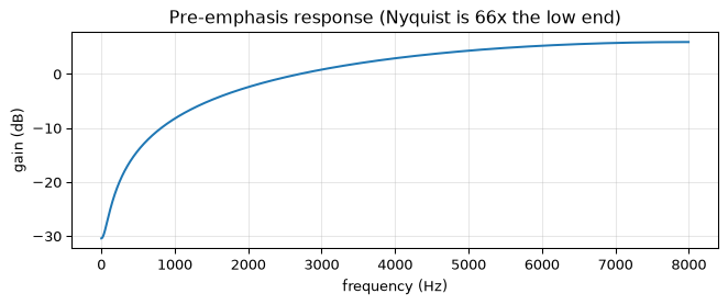
Voiced speech loses about 6 dB per octave above a few hundred Hz, an artefact of how the glottal source rolls off. Left alone, the high formants that distinguish one vowel from another arrive faint and get swamped. Pre-emphasis is the cheapest possible fix: a single-tap high-pass, $y[n] = x[n] - \alpha\,x[n-1]$ with $\alpha \approx 0.97$, whose rising response cancels the source tilt before the filterbank ever sees the signal.

w, h = freqz([1.0, -0.97], worN=2048, fs=fs)
tilt = abs(h[-1]) / abs(h[1])          # Nyquist gain over the lowest bin
assert tilt > 20                       # a genuine high-pass tilt, not flat

plt.figure(figsize=(7, 3))
plt.plot(w, 20 * np.log10(np.abs(h) + 1e-9))
plt.xlabel("frequency (Hz)"); plt.ylabel("gain (dB)")
plt.title(f"Pre-emphasis response (Nyquist is {tilt:.0f}x the low end)")
plt.grid(alpha=0.3); plt.tight_layout(); plt.show()

Figure 1: The pre-emphasis filter $1 - 0.97 z^{-1}$: a gentle high-pass that lifts the top of the band by tens of dB before the spectrum is measured.

It is a blunt instrument and a slightly old-fashioned one (some modern front ends drop it), but it costs one multiply and one subtract per sample and it measurably balances the band energies, so it has stuck around.

Framing, windowing, and the power spectrum

Speech is only stationary for a few tens of milliseconds, so MFCCs are computed frame by frame: take a ~25 ms slice, taper it with a Hamming window to control leakage, and compute its power spectrum. This is the STFT machinery, reused wholesale, so we do not repeat it here. The output of this stage is one short-time power spectrum per frame. What is new starts when we decide how to summarise that spectrum, and the first decision is to stop measuring frequency in Hz.

The mel filterbank: hearing is not linear in Hz

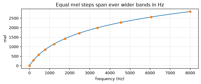
Human pitch perception is roughly linear at low frequencies and roughly logarithmic high up: the gap from 200 to 300 Hz is easy to hear, the gap from 7000 to 7100 Hz is almost inaudible. The mel scale captures this (Stevens, Volkmann, and Newman 1937). We use the common closed-form approximation (O’Shaughnessy 1987)

\[ m(f) = 2595 \, \log_{10}\!\left(1 + \frac{f}{700}\right), \]

tuned so that 1000 Hz maps to about 1000 mel.

f = np.linspace(0, 8000, 400)
assert np.isclose(hz_to_mel(1000), 1000.0, atol=1.5)     # the anchor point

centres_mel = np.linspace(0, hz_to_mel(8000), 11)
centres_hz = mel_to_hz(centres_mel)
gaps = np.diff(centres_hz)
assert gaps[-1] > 3 * gaps[0]                             # equal mel = widening Hz

plt.figure(figsize=(7, 3))
plt.plot(f, hz_to_mel(f))
plt.plot(centres_hz, centres_mel, "o", ms=5)
plt.xlabel("frequency (Hz)"); plt.ylabel("mel")
plt.title("Equal mel steps span ever wider bands in Hz"); plt.grid(alpha=0.3)
plt.tight_layout(); plt.show()

Figure 2: The mel warp. Centres placed at equal mel steps (dots) crowd together at low frequency and stretch apart high up, putting more resolution where the ear has more.

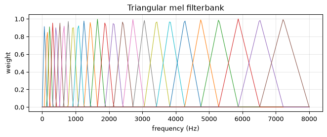
To turn the power spectrum into mel-band energies we lay a bank of triangular windows along the mel axis (equal width in mel, so widening in Hz) and take a weighted sum of the FFT bins under each triangle. The result is one number per band: the energy the ear would assign to that critical band.

fb = mel_filterbank(26, n_fft=512, fs=fs)
freqs = np.fft.rfftfreq(512, 1.0 / fs)
centres = freqs[fb.argmax(axis=1)]
assert np.all(np.diff(centres) > 0)            # centres march up in frequency
assert centres[-1] - centres[-2] > centres[1] - centres[0]   # and spread out

plt.figure(figsize=(7, 3))
for row in fb:
    plt.plot(freqs, row, lw=0.8)
plt.xlabel("frequency (Hz)"); plt.ylabel("weight")
plt.title("Triangular mel filterbank"); plt.grid(alpha=0.3)
plt.tight_layout(); plt.show()

Figure 3: A 26-band mel filterbank over a 512-point FFT at 16 kHz. The triangles are narrow and dense at the bottom, broad and sparse at the top.

The log: from a product to a sum

A speech spectrum is, to a good approximation, the product of a slowly-varying vocal-tract envelope and a fast-varying excitation. Taking the logarithm of each band energy turns that product into a sum, which is the whole point of the cepstrum: a sum is something a linear transform can pull apart. The log does double duty as perceptual compression too, since loudness is roughly logarithmic, but the algebraic reason is the one that matters for the next step.

It is worth seeing the additive structure directly. Scale the input and every log-band energy shifts by the same constant, the log of the gain, identically across all bands:

v = make_vowel()
lm1 = log_mel_spectrogram(v, fs)
lm2 = log_mel_spectrogram(2.0 * v, fs)         # double amplitude -> 4x power
shift = lm2 - lm1
assert np.allclose(shift, np.log(4.0), atol=1e-6)   # a constant offset everywhere
print(f"doubling the amplitude shifts every log-mel band by exactly "
      f"log(4) = {np.log(4):.4f} (natural-log units)")

doubling the amplitude shifts every log-mel band by exactly log(4) = 1.3863 (natural-log units)

That a level change becomes a constant offset across bands is the seed of the next idea: if the loudness lives in a single common component, a transform that isolates that component can separate “how loud” from “what shape”.

The DCT: decorrelating the bands

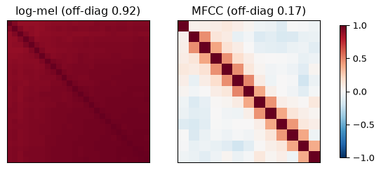
Neighbouring mel bands are strongly correlated. A formant is wide, so when one band rises its neighbours rise too, and a shared loudness sits on top of all of them. A classifier handed the raw log-mel energies has to cope with all that redundancy. The discrete cosine transform removes it. Applied across the bands, the DCT-II rewrites the log-mel envelope as a sum of cosine ripples of increasing frequency, and for the smooth, correlated envelopes speech produces, those cosine coefficients come out nearly uncorrelated. The MFCCs are those coefficients.

rng = np.random.default_rng(5)
t = np.arange(4 * fs) / fs
env = 1.0 + 0.9 * np.sin(2 * np.pi * 2.0 * t)      # slow common level drift
x = env * rng.standard_normal(t.size)
log_mel = log_mel_spectrogram(x, fs, n_filters=26)
cep = dct2(log_mel, axis=-1)[:, :13]

def offdiag_rms(M):
    c = np.corrcoef(M, rowvar=False)
    return np.sqrt(np.mean((c - np.diag(np.diag(c))) ** 2))

r_mel, r_cep = offdiag_rms(log_mel), offdiag_rms(cep)
assert r_cep < r_mel                               # the DCT decorrelates

fig, ax = plt.subplots(1, 2, figsize=(7.5, 3.2))
for a, M, title in ((ax[0], log_mel, f"log-mel (off-diag {r_mel:.2f})"),
                    (ax[1], cep, f"MFCC (off-diag {r_cep:.2f})")):
    im = a.imshow(np.corrcoef(M, rowvar=False), vmin=-1, vmax=1, cmap="RdBu_r")
    a.set_title(title); a.set_xticks([]); a.set_yticks([])
fig.colorbar(im, ax=ax, shrink=0.8); plt.show()

Figure 4: Inter-band correlation before and after the DCT, for a signal with a drifting overall level. The log-mel bands (left) are nearly all positively correlated; the MFCCs (right) are close to diagonal.

The DCT also compacts the energy: a smooth envelope is captured almost entirely by its first handful of coefficients, which is why we keep only the low-order ones (typically 13) and discard the rest. The discarded high-order coefficients describe the fine, pitch-related ripple, exactly the part we wanted to drop.

env_logmel = log_mel_spectrogram(make_vowel(), fs).mean(axis=0)
c = dct2(env_logmel)
frac = np.sum(c[:6] ** 2) / np.sum(c ** 2)
assert frac > 0.9                                  # first 6 of 26 hold the envelope
print(f"the first 6 of 26 DCT coefficients carry {100*frac:.0f}% of the "
      f"log-mel envelope's energy")

the first 6 of 26 DCT coefficients carry 94% of the log-mel envelope's energy

Which cosine transform, and why a cosine at all

The cosine transform is a family. Visualised on the frequency circle, each variant samples a slightly different set of basis frequencies; a generalised-transforms course demo that motivated this section plotted the DCT-IV and DST-IV grids that way. MFCC uses the type-II DCT, whose orthonormal basis cosines sit at $k$ multiples of $\pi/N$ and whose first vector is the flat (DC) term that absorbs the overall loudness. A real cosine transform (rather than a full Fourier transform) is the right tool here because the log-mel envelope is real and symmetric-friendly, and the DCT-II is the transform that best approximates the optimal decorrelating (Karhunen-Loeve) transform for the smooth, positively-correlated signals speech produces.

Deltas: how the coefficients move

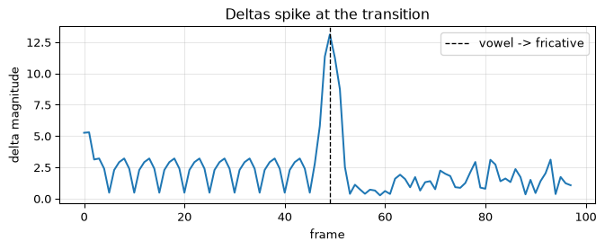
A static MFCC vector says nothing about motion, yet a plosive bursting open or a vowel gliding into a consonant is defined by change. The fix is to append delta (velocity) and delta-delta (acceleration) coefficients: a short regression of each coefficient track against time. Stacking the 13 static coefficients with 13 deltas and 13 delta-deltas gives the classic 39-dimensional speech feature.

sig = np.concatenate([make_vowel(0.5), make_fricative(0.5)])
coeffs = mfcc(sig, fs)
d = delta(coeffs)
dmag = np.linalg.norm(d, axis=1)
mid = coeffs.shape[0] // 2
assert abs(int(dmag.argmax()) - mid) <= 3          # the spike is at the boundary

plt.figure(figsize=(7, 3))
plt.plot(dmag)
plt.axvline(mid, color="k", ls="--", lw=1, label="vowel -> fricative")
plt.xlabel("frame"); plt.ylabel("delta magnitude")
plt.title("Deltas spike at the transition"); plt.legend(); plt.grid(alpha=0.3)
plt.tight_layout(); plt.show()

Figure 5: Delta magnitude across a sound that switches from a vowel to a fricative halfway through. The deltas are quiet while each sound is steady and spike at the transition.

Three sounds, three fingerprints

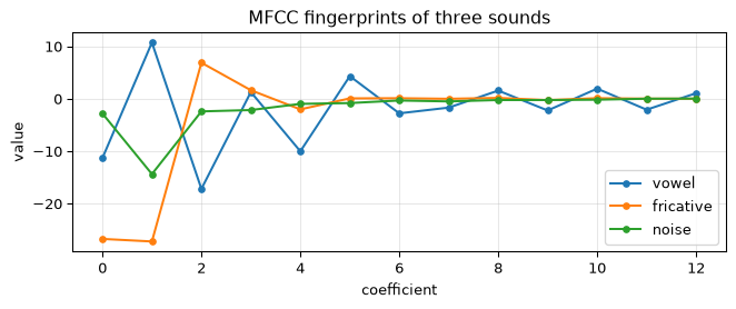
The payoff is that very different sounds land at very different points in MFCC space, which is what lets a downstream classifier separate them. Averaged over a held tone, a fricative, and white noise, the mean MFCC vectors are plainly distinct.

import itertools
def mean_mfcc(x):
    return mfcc(x, fs).mean(axis=0)

vecs = {"vowel": mean_mfcc(make_vowel()),
        "fricative": mean_mfcc(make_fricative()),
        "noise": mean_mfcc(make_noise())}
dists = [np.linalg.norm(a - b) for a, b in itertools.combinations(vecs.values(), 2)]
assert min(dists) > 5.0                             # every pair is well separated

plt.figure(figsize=(7, 3))
for name, vec in vecs.items():
    plt.plot(vec, "o-", ms=4, label=name)
plt.xlabel("coefficient"); plt.ylabel("value")
plt.title("MFCC fingerprints of three sounds"); plt.legend(); plt.grid(alpha=0.3)
plt.tight_layout(); plt.show()

Figure 6: Mean MFCC vectors for a voiced vowel, a fricative, and white noise. The low coefficients already pull the three sounds apart.

This separability is exactly what the wakeword detector on hardware exploits: compute MFCCs in C on an ESP32-S3, and match them against a few stored reference utterances with dynamic time warping. No training, no network, a few kilobytes of state.

Going further

The MFCC is a beautiful piece of classical engineering, and it is honest to say where it strains.

It is fragile to noise and channel. The log makes additive noise behave badly, and a different microphone or room shifts the cepstrum. Real systems lean on cepstral mean normalisation, deltas, and more to cope, and still degrade in the wild.
It discards phase and most pitch. That is deliberate (it is what makes the envelope compact), but it means MFCCs cannot tell two speakers apart by pitch, and they throw away cues some tasks need.
The mel filterbank and DCT are fixed, not learned. Modern speech systems increasingly feed a network the log-mel spectrogram directly, or even the waveform, and let it learn the equivalent of the DCT and more. When there is data to learn from, learned features usually win.
The choices are conventional, not optimal. The number of filters, the number of coefficients kept, the pre-emphasis value, the mel formula itself: all are defaults that work well, not derived optima. Treat them as starting points.

Where MFCC still earns its place is exactly where this workshop lives: small, training-free, real-time classifiers on hardware that cannot run a network. The embedded page builds one, and its closing “what next” points at the TinyML and Edge Impulse path for when a learned model is worth the silicon.

References

Davis, Steven B., and Paul Mermelstein. 1980. “Comparison of Parametric Representations for Monosyllabic Word Recognition in Continuously Spoken Sentences.” IEEE Transactions on Acoustics, Speech, and Signal Processing 28 (4): 357–66.

O’Shaughnessy, Douglas. 1987. Speech Communication: Human and Machine. Addison-Wesley.

Rabiner, Lawrence R., and Biing-Hwang Juang. 1993. Fundamentals of Speech Recognition. Prentice Hall.

Stevens, Stanley Smith, John Volkmann, and Edwin B. Newman. 1937. “A Scale for the Measurement of the Psychological Magnitude Pitch.” Journal of the Acoustical Society of America 8 (3): 185–90.

--- title: "Mel-Frequency Cepstral Coefficients" subtitle: "Turning a spectrum into a short, decorrelated fingerprint of a sound" bibliography: ../../references.bib --- Ask a spectrogram what a vowel sounds like and it hands you hundreds of numbers per frame, most of them redundant. Ask an [MFCC](mfcc.py) front end the same question and it hands you thirteen. Those thirteen numbers describe the *shape of the spectral envelope*, warped to match how human hearing resolves frequency and decorrelated so a simple classifier can use them directly. This compression is why the MFCC was the feature behind a generation of speech recognisers [@davis1980comparison; @rabiner1993fundamentals], and why it still anchors small keyword spotters that have to run on a coin cell. This page is the practitioner's walk through the pipeline. It is a fixed sequence of small, cheap steps, and the interesting part is *what each one is for* and *what it throws away*. We build it on top of the two topics before it: the [STFT](../stft/index.qmd) supplies the framing and the per-frame spectrum, and the [spectral features](../spectral-features/index.qmd) page is the sibling that summarises that spectrum a different way. MFCC is the speech-flavoured cousin. ::: {.callout-note title="Prerequisites"} This builds on the [STFT](../stft/index.qmd) (framing, windowing, the per-frame spectrum) and reads naturally after [spectral features](../spectral-features/index.qmd). The clean, importable code is in [`mfcc.py`](mfcc.py), checked by [`test_mfcc.py`](test_mfcc.py). The embedded companion, [a wakeword detector on the metal](embedded.qmd), turns this front end into a working classifier. ::: ```{python} #| echo: false import numpy as np import matplotlib.pyplot as plt from scipy.signal import butter, lfilter, freqz from mfcc import ( hz_to_mel, mel_to_hz, pre_emphasis, frame_signal, power_spectrum, mel_filterbank, log_mel_spectrogram, dct2, mfcc, delta, ) fs = 16000 def make_vowel(dur=1.0, f0=120.0, seed=None): """A synthetic voiced vowel: a harmonic stack shaped by two formants.""" t = np.arange(int(dur * fs)) / fs x = np.zeros_like(t) for k in range(1, 40): fk = k * f0 if fk >= fs / 2: break env = (np.exp(-((fk - 700) / 400) ** 2) + 0.7 * np.exp(-((fk - 1200) / 500) ** 2) + 0.05) x += env * np.sin(2 * np.pi * fk * t) return x def make_fricative(dur=1.0, seed=1): """A synthetic fricative: high-pass-filtered noise, energy up top.""" rng = np.random.default_rng(seed) b, a = butter(4, 4000 / (fs / 2), "high") return lfilter(b, a, rng.standard_normal(int(dur * fs))) def make_noise(dur=1.0, seed=2): return np.random.default_rng(seed).standard_normal(int(dur * fs)) ``` ## The pipeline at a glance An MFCC vector is built by passing each short frame of audio through a fixed chain: 1. **Pre-emphasis**: a one-tap high-pass that boosts the weak high frequencies of voiced speech. 2. **Framing and windowing**: cut into ~25 ms frames at a ~10 ms hop, taper each one. This is exactly the [STFT](../stft/index.qmd) front end. 3. **Power spectrum**: the periodogram of each frame. 4. **Mel filterbank**: sum that power into a couple of dozen perceptually-spaced bands. 5. **Log**: take the logarithm of each band energy. 6. **DCT**: a discrete cosine transform that decorrelates the log-band energies; keep the low-order coefficients. 7. **Deltas** (optional): append first and second time differences to capture how the coefficients move. The first half (steps 1 to 5) is the *cepstral* idea borrowed from speech analysis: separate the slowly-varying vocal-tract envelope from the fast pitch detail. The DCT in step 6 is the twist that makes the result compact and uncorrelated. We take the steps in order. ## Pre-emphasis: tilting the spectrum back up Voiced speech loses about 6 dB per octave above a few hundred Hz, an artefact of how the glottal source rolls off. Left alone, the high formants that distinguish one vowel from another arrive faint and get swamped. Pre-emphasis is the cheapest possible fix: a single-tap high-pass, $y[n] = x[n] - \alpha\,x[n-1]$ with $\alpha \approx 0.97$, whose rising response cancels the source tilt before the filterbank ever sees the signal. ```{python} #| label: fig-preemph #| fig-cap: "The pre-emphasis filter $1 - 0.97 z^{-1}$: a gentle high-pass that lifts the top of the band by tens of dB before the spectrum is measured." w, h = freqz([1.0, -0.97], worN=2048, fs=fs) tilt = abs(h[-1]) / abs(h[1]) # Nyquist gain over the lowest bin assert tilt > 20 # a genuine high-pass tilt, not flat plt.figure(figsize=(7, 3)) plt.plot(w, 20 * np.log10(np.abs(h) + 1e-9)) plt.xlabel("frequency (Hz)"); plt.ylabel("gain (dB)") plt.title(f"Pre-emphasis response (Nyquist is {tilt:.0f}x the low end)") plt.grid(alpha=0.3); plt.tight_layout(); plt.show() ``` It is a blunt instrument and a slightly old-fashioned one (some modern front ends drop it), but it costs one multiply and one subtract per sample and it measurably balances the band energies, so it has stuck around. ## Framing, windowing, and the power spectrum Speech is only stationary for a few tens of milliseconds, so MFCCs are computed frame by frame: take a ~25 ms slice, taper it with a Hamming window to control leakage, and compute its power spectrum. This is the [STFT](../stft/index.qmd) machinery, reused wholesale, so we do not repeat it here. The output of this stage is one short-time power spectrum per frame. What is new starts when we decide *how to summarise* that spectrum, and the first decision is to stop measuring frequency in Hz. ## The mel filterbank: hearing is not linear in Hz Human pitch perception is roughly linear at low frequencies and roughly logarithmic high up: the gap from 200 to 300 Hz is easy to hear, the gap from 7000 to 7100 Hz is almost inaudible. The **mel scale** captures this [@stevens1937scale]. We use the common closed-form approximation [@oshaughnessy1987speech] $$ m(f) = 2595 \, \log_{10}\!\left(1 + \frac{f}{700}\right), $$ tuned so that 1000 Hz maps to about 1000 mel. ```{python} #| label: fig-mel #| fig-cap: "The mel warp. Centres placed at equal mel steps (dots) crowd together at low frequency and stretch apart high up, putting more resolution where the ear has more." f = np.linspace(0, 8000, 400) assert np.isclose(hz_to_mel(1000), 1000.0, atol=1.5) # the anchor point centres_mel = np.linspace(0, hz_to_mel(8000), 11) centres_hz = mel_to_hz(centres_mel) gaps = np.diff(centres_hz) assert gaps[-1] > 3 * gaps[0] # equal mel = widening Hz plt.figure(figsize=(7, 3)) plt.plot(f, hz_to_mel(f)) plt.plot(centres_hz, centres_mel, "o", ms=5) plt.xlabel("frequency (Hz)"); plt.ylabel("mel") plt.title("Equal mel steps span ever wider bands in Hz"); plt.grid(alpha=0.3) plt.tight_layout(); plt.show() ``` To turn the power spectrum into mel-band energies we lay a bank of triangular windows along the mel axis (equal width in mel, so widening in Hz) and take a weighted sum of the FFT bins under each triangle. The result is one number per band: the energy the ear would assign to that critical band. ```{python} #| label: fig-filterbank #| fig-cap: "A 26-band mel filterbank over a 512-point FFT at 16 kHz. The triangles are narrow and dense at the bottom, broad and sparse at the top." fb = mel_filterbank(26, n_fft=512, fs=fs) freqs = np.fft.rfftfreq(512, 1.0 / fs) centres = freqs[fb.argmax(axis=1)] assert np.all(np.diff(centres) > 0) # centres march up in frequency assert centres[-1] - centres[-2] > centres[1] - centres[0] # and spread out plt.figure(figsize=(7, 3)) for row in fb: plt.plot(freqs, row, lw=0.8) plt.xlabel("frequency (Hz)"); plt.ylabel("weight") plt.title("Triangular mel filterbank"); plt.grid(alpha=0.3) plt.tight_layout(); plt.show() ``` ## The log: from a product to a sum A speech spectrum is, to a good approximation, the *product* of a slowly-varying vocal-tract envelope and a fast-varying excitation. Taking the logarithm of each band energy turns that product into a *sum*, which is the whole point of the cepstrum: a sum is something a linear transform can pull apart. The log does double duty as perceptual compression too, since loudness is roughly logarithmic, but the algebraic reason is the one that matters for the next step. It is worth seeing the additive structure directly. Scale the input and every log-band energy shifts by the same constant, the log of the gain, identically across all bands: ```{python} #| label: log-additive v = make_vowel() lm1 = log_mel_spectrogram(v, fs) lm2 = log_mel_spectrogram(2.0 * v, fs) # double amplitude -> 4x power shift = lm2 - lm1 assert np.allclose(shift, np.log(4.0), atol=1e-6) # a constant offset everywhere print(f"doubling the amplitude shifts every log-mel band by exactly " f"log(4) = {np.log(4):.4f} (natural-log units)") ``` That a level change becomes a *constant* offset across bands is the seed of the next idea: if the loudness lives in a single common component, a transform that isolates that component can separate "how loud" from "what shape". ## The DCT: decorrelating the bands Neighbouring mel bands are strongly correlated. A formant is wide, so when one band rises its neighbours rise too, and a shared loudness sits on top of all of them. A classifier handed the raw log-mel energies has to cope with all that redundancy. The **discrete cosine transform** removes it. Applied across the bands, the DCT-II rewrites the log-mel envelope as a sum of cosine ripples of increasing frequency, and for the smooth, correlated envelopes speech produces, those cosine coefficients come out nearly uncorrelated. The MFCCs *are* those coefficients. ```{python} #| label: fig-decorrelate #| fig-cap: "Inter-band correlation before and after the DCT, for a signal with a drifting overall level. The log-mel bands (left) are nearly all positively correlated; the MFCCs (right) are close to diagonal." rng = np.random.default_rng(5) t = np.arange(4 * fs) / fs env = 1.0 + 0.9 * np.sin(2 * np.pi * 2.0 * t) # slow common level drift x = env * rng.standard_normal(t.size) log_mel = log_mel_spectrogram(x, fs, n_filters=26) cep = dct2(log_mel, axis=-1)[:, :13] def offdiag_rms(M): c = np.corrcoef(M, rowvar=False) return np.sqrt(np.mean((c - np.diag(np.diag(c))) ** 2)) r_mel, r_cep = offdiag_rms(log_mel), offdiag_rms(cep) assert r_cep < r_mel # the DCT decorrelates fig, ax = plt.subplots(1, 2, figsize=(7.5, 3.2)) for a, M, title in ((ax[0], log_mel, f"log-mel (off-diag {r_mel:.2f})"), (ax[1], cep, f"MFCC (off-diag {r_cep:.2f})")): im = a.imshow(np.corrcoef(M, rowvar=False), vmin=-1, vmax=1, cmap="RdBu_r") a.set_title(title); a.set_xticks([]); a.set_yticks([]) fig.colorbar(im, ax=ax, shrink=0.8); plt.show() ``` The DCT also *compacts* the energy: a smooth envelope is captured almost entirely by its first handful of coefficients, which is why we keep only the low-order ones (typically 13) and discard the rest. The discarded high-order coefficients describe the fine, pitch-related ripple, exactly the part we wanted to drop. ```{python} #| label: compaction env_logmel = log_mel_spectrogram(make_vowel(), fs).mean(axis=0) c = dct2(env_logmel) frac = np.sum(c[:6] ** 2) / np.sum(c ** 2) assert frac > 0.9 # first 6 of 26 hold the envelope print(f"the first 6 of 26 DCT coefficients carry {100*frac:.0f}% of the " f"log-mel envelope's energy") ``` ::: {.callout-note title="Which cosine transform, and why a cosine at all"} The cosine transform is a family. Visualised on the frequency circle, each variant samples a slightly different set of basis frequencies; a generalised-transforms course demo that motivated this section plotted the DCT-IV and DST-IV grids that way. MFCC uses the **type-II** DCT, whose orthonormal basis cosines sit at $k$ multiples of $\pi/N$ and whose first vector is the flat (DC) term that absorbs the overall loudness. A real cosine transform (rather than a full Fourier transform) is the right tool here because the log-mel envelope is real and symmetric-friendly, and the DCT-II is the transform that best approximates the optimal decorrelating (Karhunen-Loeve) transform for the smooth, positively-correlated signals speech produces. ::: ## Deltas: how the coefficients move A static MFCC vector says nothing about *motion*, yet a plosive bursting open or a vowel gliding into a consonant is defined by change. The fix is to append **delta** (velocity) and **delta-delta** (acceleration) coefficients: a short regression of each coefficient track against time. Stacking the 13 static coefficients with 13 deltas and 13 delta-deltas gives the classic 39-dimensional speech feature. ```{python} #| label: fig-delta #| fig-cap: "Delta magnitude across a sound that switches from a vowel to a fricative halfway through. The deltas are quiet while each sound is steady and spike at the transition." sig = np.concatenate([make_vowel(0.5), make_fricative(0.5)]) coeffs = mfcc(sig, fs) d = delta(coeffs) dmag = np.linalg.norm(d, axis=1) mid = coeffs.shape[0] // 2 assert abs(int(dmag.argmax()) - mid) <= 3 # the spike is at the boundary plt.figure(figsize=(7, 3)) plt.plot(dmag) plt.axvline(mid, color="k", ls="--", lw=1, label="vowel -> fricative") plt.xlabel("frame"); plt.ylabel("delta magnitude") plt.title("Deltas spike at the transition"); plt.legend(); plt.grid(alpha=0.3) plt.tight_layout(); plt.show() ``` ## Three sounds, three fingerprints The payoff is that very different sounds land at very different points in MFCC space, which is what lets a downstream classifier separate them. Averaged over a held tone, a fricative, and white noise, the mean MFCC vectors are plainly distinct. ```{python} #| label: fig-fingerprints #| fig-cap: "Mean MFCC vectors for a voiced vowel, a fricative, and white noise. The low coefficients already pull the three sounds apart." import itertools def mean_mfcc(x): return mfcc(x, fs).mean(axis=0) vecs = {"vowel": mean_mfcc(make_vowel()), "fricative": mean_mfcc(make_fricative()), "noise": mean_mfcc(make_noise())} dists = [np.linalg.norm(a - b) for a, b in itertools.combinations(vecs.values(), 2)] assert min(dists) > 5.0 # every pair is well separated plt.figure(figsize=(7, 3)) for name, vec in vecs.items(): plt.plot(vec, "o-", ms=4, label=name) plt.xlabel("coefficient"); plt.ylabel("value") plt.title("MFCC fingerprints of three sounds"); plt.legend(); plt.grid(alpha=0.3) plt.tight_layout(); plt.show() ``` This separability is exactly what the [wakeword detector on hardware](embedded.qmd) exploits: compute MFCCs in C on an ESP32-S3, and match them against a few stored reference utterances with dynamic time warping. No training, no network, a few kilobytes of state. ## Going further The MFCC is a beautiful piece of classical engineering, and it is honest to say where it strains. - **It is fragile to noise and channel.** The log makes additive noise behave badly, and a different microphone or room shifts the cepstrum. Real systems lean on cepstral mean normalisation, deltas, and more to cope, and still degrade in the wild. - **It discards phase and most pitch.** That is deliberate (it is what makes the envelope compact), but it means MFCCs cannot tell two speakers apart by pitch, and they throw away cues some tasks need. - **The mel filterbank and DCT are fixed, not learned.** Modern speech systems increasingly feed a network the log-mel spectrogram directly, or even the waveform, and let it learn the equivalent of the DCT and more. When there is data to learn from, learned features usually win. - **The choices are conventional, not optimal.** The number of filters, the number of coefficients kept, the pre-emphasis value, the mel formula itself: all are defaults that work well, not derived optima. Treat them as starting points. Where MFCC still earns its place is exactly where this workshop lives: small, training-free, real-time classifiers on hardware that cannot run a network. The [embedded page](embedded.qmd) builds one, and its closing "what next" points at the [TinyML](https://www.tinyml.org/) and Edge Impulse path for when a learned model is worth the silicon. ## References ::: {#refs} :::