Watching a spectrum change, and putting the signal back together again
A single Fourier transform answers one question: which frequencies are in this signal? It assumes the answer does not change while you are listening. For a steady tone that is fine. For speech, music, a bird call, an engine running up through its gears, or a radar echo, it is the wrong question. The frequencies are moving, and a single spectrum averages that motion into a blur.
The Short-Time Fourier Transform (STFT) asks a better question: which frequencies are present right now, and now, and now? It does this by chopping the signal into short frames, windowing each one, and taking its DFT. Stack those spectra side by side and you get a time-frequency picture: the data behind every spectrogram you have ever seen.
This page is the practitioner’s tour of that idea. The intuition, the window functions, and the leakage they fight are already covered in the basics; here we go to the parts a first pass skips: the resolution trade-off you cannot escape, how much frames should overlap, and how to invert the transform and get your signal back.
The implementation is stft.py. Save test_stft.py beside it and pytest test_stft.py runs the checks on it.
From one spectrum to many
The recipe is mechanical. Slide a window of length \(L\) along the signal in steps of \(H\) samples (the hop). At each position \(m\), multiply the \(L\) samples under the window by a window function \(w\), and take the DFT:
\[X[m, k] = \sum_{n=0}^{L-1} w[n]\,x[mH + n]\,e^{-j 2\pi k n / L}.\]
Two indices now, not one. The bin index \(k\) is frequency, exactly as in an ordinary DFT, with bin spacing \(\Delta f = f_s / L\). The frame index \(m\) is time: frame \(m\) is centred at sample \(mH + L/2\), so consecutive columns of the result are \(H/f_s\) seconds apart. The magnitude \(|X[m,k]|^2\), drawn as an image with time across and frequency up, is the spectrogram.
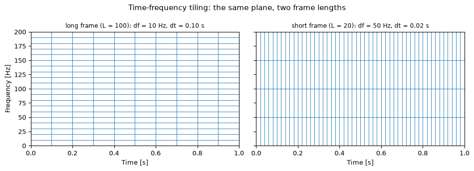
Figure 1: The STFT lays a grid over the time-frequency plane. Each tile is one DFT bin of one frame: its width is the frame duration, its height is the bin spacing. A long frame makes wide, short tiles (fine in frequency, coarse in time); a short frame makes narrow, tall ones (coarse in frequency, fine in time). Every tile has the same unit area.
That picture already contains the central tension of the whole subject. The total area of each tile is fixed at \(\Delta t \cdot \Delta f = (L/f_s)(f_s/L) = 1\). This exact equality is the grid-level face of the uncertainty principle: that bound, \(\Delta t \cdot \Delta f \geq 1\), limits how tightly any atom can be concentrated, while here it lands on equality because every tile is pinned to the same frame length \(L\), so \(L/f_s\) and \(f_s/L\) cancel by construction. You can make the tiles wide and short or narrow and tall, but you cannot make them small. Choosing the frame length is choosing how to spend that fixed budget between time and frequency. Hold a tone still long enough to measure its pitch exactly, and the moment it belonged to has already slipped past.
The resolution trade-off: narrowband versus wideband
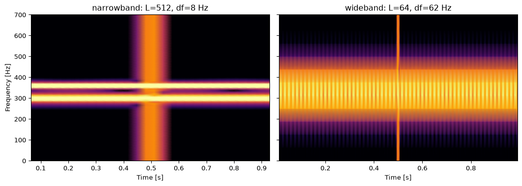
This is the decision that matters, so it is worth seeing fail in both directions. Take a signal that genuinely needs both kinds of resolution: two steady tones only 60 Hz apart (to tell them apart you need fine frequency resolution) plus a sharp click halfway through (to place it you need fine time resolution).
Show the code
fs, dur =4000.0, 1.0t = np.arange(int(fs * dur)) / fsf1, f2 =300.0, 360.0x = np.sin(2* np.pi * f1 * t) + np.sin(2* np.pi * f2 * t)x[int(0.5* fs)] +=8.0# a sharp transientn_long, n_short =512, 64df_long, df_short = fs / n_long, fs / n_shortdt_long, dt_short = n_long / fs, n_short / fs# the long frame resolves the 60 Hz gap; the short frame resolves the clickassert df_long <60< df_shortassert dt_short <0.05< dt_longfig, axes = plt.subplots(1, 2, figsize=(11, 4), sharey=True)for ax, (L, name) inzip(axes, [(n_long, f'narrowband: L={n_long}, df={df_long:.0f} Hz'), (n_short, f'wideband: L={n_short}, df={df_short:.0f} Hz')]): f, tt, S = spectrogram(x, fs, 'hann', L, L *3//4) ax.pcolormesh(tt, f, 10* np.log10(S +1e-6), shading='gouraud', cmap='inferno', vmin=-20, vmax=30) ax.set_xlabel('Time [s]'); ax.set_title(name); ax.set_ylim(0, 700)axes[0].set_ylabel('Frequency [Hz]')fig.tight_layout()plt.show()# verify the trade-off numerically: count resolved tone-peaks away from the clickdef tone_peaks(L): f, tt, S = spectrogram(x, fs, 'hann', L, L //2) spec = S[:, (tt >0.1) & (tt <0.4)].mean(axis=1) band = (f >=250) & (f <=420) fb, sb = f[band], spec[band]return [fb[i] for i inrange(1, len(sb) -1)if sb[i] > sb[i -1] and sb[i] > sb[i +1] and sb[i] >0.05* sb.max()]assertlen(tone_peaks(n_long)) ==2# narrowband splits the tonesassertlen(tone_peaks(n_short)) ==1# wideband merges themprint(f"narrowband peaks: {np.round(tone_peaks(n_long), 0)} Hz (two tones resolved)")print(f"wideband peaks: {np.round(tone_peaks(n_short), 0)} Hz (merged into one)")
Figure 2: The same signal (two tones 60 Hz apart, plus a click at 0.5 s) under a long frame and a short frame. The long frame (narrowband) splits the two tones but smears the click into a vertical streak; the short frame (wideband) pins the click in time but merges the tones into one ridge. No single frame length wins.
The names come from speech analysis. A narrowband spectrogram uses a long frame (tens of milliseconds), resolving individual harmonics as horizontal lines but blurring fast events. A wideband spectrogram uses a short frame (a few milliseconds), resolving each glottal pulse as a vertical striation but merging the harmonics into formant bands. Speech scientists keep both on screen because each shows what the other hides. There is no universally correct frame length; there is only the question you are asking. If you need both at once, that is exactly the itch the wavelet transform scratches, by letting the tile shape vary with frequency.
Overlap, hop, and redundancy
Why slide the window in small steps instead of laying frames end to end? Because a tapered window throws away the samples near its edges, where it falls to zero. With no overlap (\(H = L\)), an event that lands at a frame boundary is attenuated by both neighbouring frames and barely registers. Overlapping the frames means every sample sits near the centre of some frame.
The hop is usually quoted as an overlap fraction: 50% overlap is \(H = L/2\), 75% is \(H = L/4\). More overlap gives a smoother spectrogram and better time localisation of the analysis, at a proportional cost in compute and storage, since you produce more frames. For analysis-only spectrograms, 50% to 75% is the usual range. For anything you intend to invert, the hop is not a free choice: it has to satisfy a condition.
Inverting the STFT: overlap-add and the COLA condition
The STFT is invertible. Take the inverse DFT of each frame to recover the windowed time slices, lay them back down at their original positions, and add the overlaps. The only subtlety is the window: each output sample has been multiplied by whatever window values covered it, so you divide by the sum of those windows. That is windowed overlap-add, and it reconstructs the signal exactly wherever the frames cover it, for any window:
Show the code
fs =4000.0rng = np.random.default_rng(0)x = np.cumsum(rng.standard_normal(6000)) *0.05# a wandering test signalx += np.sin(2* np.pi *200* np.arange(len(x)) / fs)f, tt, Z = stft(x, fs, 'hann', 256, 128)_, xr = istft(Z, fs, 'hann', 256, 128)interior =slice(256, len(xr) -256) # where every sample is coverederr = np.max(np.abs(xr[interior] - x[interior]))assert err <1e-9print(f"max reconstruction error on the interior: {err:.2e} (exact, to rounding)")
max reconstruction error on the interior: 3.55e-15 (exact, to rounding)
So why does anyone talk about a special condition? Because dividing by the window sum, sample by sample, is something a real-time system would rather not do, and because the moment you modify the spectrogram (zero out a noisy region, apply a gain mask, denoise) the clean “divide it back out” identity no longer holds: there is no single signal whose STFT is your modified array. What saves you is choosing a window and hop for which the shifted windows already add up to a constant. That is the Constant-OverLap-Add (COLA) condition:
\[\sum_{m} w[n - mH] = C \quad \text{for all } n.\]
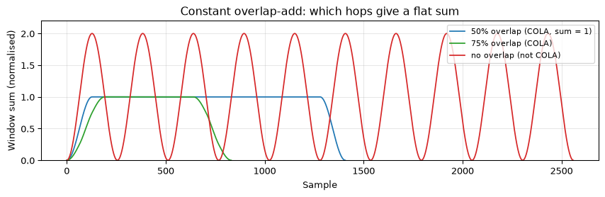
When COLA holds, overlap-add reconstruction is just a fixed gain \(C\) with no per-sample division, and a modified spectrogram resynthesises into the signal whose frames are closest to your modified ones, with no window-induced ripple (Allen and Rabiner 1977; Griffin and Lim 1984). The textbook case is a Hann window at 50% overlap, which sums to exactly 1. The same Hann window with no overlap does not: it dips to zero between frames.
Show the code
ok_half, c_half = cola('hann', 256, 128)ok_75, c_75 = cola('hann', 256, 192)ok_none, _ = cola('hann', 256, 0)assert ok_half and np.isclose(c_half, 1.0) # Hann + 50% overlap: COLA, C = 1assert ok_75 and np.isclose(c_75, 2.0) # Hann + 75% overlap: COLA, C = 2assertnot ok_none # Hann + no overlap: not COLAfrom scipy.signal import get_windoww = get_window('hann', 256, fftbins=True)fig, ax = plt.subplots(figsize=(9, 3))for noverlap, label, color in [(128, '50% overlap (COLA, sum = 1)', 'C0'), (192, '75% overlap (COLA)', 'C2'), (0, 'no overlap (not COLA)', 'C3')]: hop =256- noverlap nf =10 s = np.zeros((nf -1) * hop +256)for i inrange(nf): s[i * hop:i * hop +256] += w norm = s / (s[256:-256].mean()) # normalise steady-state to 1 ax.plot(norm, color=color, lw=1.3, label=label)ax.set_ylim(0, 2.2); ax.set_xlabel('Sample'); ax.set_ylabel('Window sum (normalised)')ax.legend(fontsize=8, loc='upper right'); ax.grid(True, alpha=0.3)ax.set_title('Constant overlap-add: which hops give a flat sum')fig.tight_layout()plt.show()
Figure 3: The overlap-add sum of the analysis windows. A Hann window at 50% overlap sums to a flat constant (COLA satisfied, C = 1); at 75% overlap it also sums flat (COLA, C = 2); with no overlap the gaps at the window edges show through as deep ripples (COLA violated).
A spectrogram, end to end
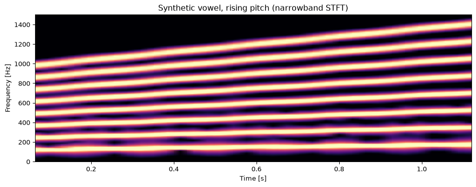
Pulling it together on a real-flavoured signal: a synthetic vowel, a harmonic stack whose pitch glides, the kind of thing the narrowband view is made for.
Figure 4: Narrowband spectrogram of a synthetic vowel with a rising pitch. The horizontal lines are the harmonics of the glottal source; their spacing widens as the pitch glides up. This is the analysis the STFT was built for.
On hardware
A spectrogram on a microcontroller is a block FFT in a loop: collect \(L\) samples, window, FFT, square, repeat with a hop. The interesting parts are the ones the desktop version hides: where the overlap buffer lives, how big \(L\) can be before it eats your RAM, and whether the FFT keeps up with the audio. Those are worked through on the embedded page for the ESP32-S3 (ESP-DSP) and the NUCLEO-F446RE (CMSIS-DSP).
Going further
Phase matters, and is hard. A spectrogram usually shows only magnitude, but the STFT carries phase too, and you need it to invert. Reconstructing a signal from a modified magnitude alone (after denoising, say) means guessing a consistent phase. The Griffin-Lim algorithm iterates between the time and frequency domains to do exactly that (Griffin and Lim 1984), and it is the classical ancestor of the vocoders inside modern audio models.
The tile shape need not be fixed. The STFT commits to one frame length for the whole signal. The wavelet transform trades that for tiles that are short at high frequencies and long at low ones, matching how real signals tend to be structured. Constant-Q transforms do the same with a logarithmic frequency axis, which is why they suit music.
Reassignment and synchrosqueezing sharpen a blurry spectrogram by moving each tile’s energy to its centre of gravity, recovering detail the fixed grid throws away, at the cost of giving up the clean invertibility above.
Where it leads here. The STFT is the front end for nearly everything that follows: per-frame spectral features (centroid, rolloff, flux), the mel filterbank and DCT behind MFCCs, and the frequency-domain forms of matched filtering and beamforming.
References
Allen, Jont B., and Lawrence R. Rabiner. 1977. “A Unified Approach to Short-Time Fourier Analysis and Synthesis.”Proceedings of the IEEE 65 (11): 1558–64.
Griffin, Daniel W., and Jae S. Lim. 1984. “Signal Estimation from Modified Short-Time Fourier Transform.”IEEE Transactions on Acoustics, Speech, and Signal Processing 32 (2): 236–43.
Harris, Fredric J. 1978. “On the Use of Windows for Harmonic Analysis with the Discrete Fourier Transform.”Proceedings of the IEEE 66 (1): 51–83.
Source Code
---title: "The Short-Time Fourier Transform"subtitle: "Watching a spectrum change, and putting the signal back together again"description-meta: "Watching a spectrum change over time: framing, windowing, hop size, the time-frequency trade-off, and getting the signal back again."bibliography: ../../references.bib---A single Fourier transform answers one question: which frequencies are in this signal? It assumes the answer does not change while you are listening. For a steady tone that is fine. For speech, music, a bird call, an engine running up through its gears, or a radar echo, it is the wrong question. The frequencies are *moving*, and a single spectrum averages that motion into a blur.The **Short-Time Fourier Transform** (STFT) asks a better question: which frequencies are present *right now*, and now, and now? It does this by chopping the signal into short frames, windowing each one, and taking its DFT. Stack those spectra side by side and you get a time-frequency picture: the data behind every spectrogram you have ever seen.This page is the practitioner's tour of that idea. The intuition, the window functions, and the leakage they fight are already covered in the basics; here we go to the parts a first pass skips: the resolution trade-off you cannot escape, how much frames should overlap, and how to invert the transform and get your signal back.::: {.callout-note title="Prerequisites"}Part of the [feature extraction arc](../feature-extraction.qmd); the overview gives the reading order.This builds directly on the [DFT, spectral leakage, and window functions](../../basics/05-frequency-domain.qmd)[@harris1978use] from the frequency-domain chapter, which also introduces [the spectrogram and the uncertainty principle](../../basics/05-frequency-domain.qmd#the-spectrogram). We lean on that material rather than repeat it.:::::: {.callout-tip title="Code"}The implementation is [`stft.py`](stft.py). Save [`test_stft.py`](test_stft.py) beside it and `pytest test_stft.py` runs the checks on it.:::```{python}#| echo: falseimport numpy as npimport matplotlib.pyplot as pltfrom stft import stft, istft, cola, spectrogram```## From one spectrum to manyThe recipe is mechanical. Slide a window of length $L$ along the signal in steps of $H$ samples (the **hop**). At each position $m$, multiply the $L$ samples under the window by a window function $w$, and take the DFT:$$X[m, k] = \sum_{n=0}^{L-1} w[n]\,x[mH + n]\,e^{-j 2\pi k n / L}.$$Two indices now, not one. The bin index $k$ is frequency, exactly as in an ordinary DFT, with bin spacing $\Delta f = f_s / L$. The frame index $m$ is time: frame $m$ is centred at sample $mH + L/2$, so consecutive columns of the result are $H/f_s$ seconds apart. The magnitude $|X[m,k]|^2$, drawn as an image with time across and frequency up, is the **spectrogram**.```{python}#| label: fig-stft-tiles#| code-fold: true#| fig-cap: "The STFT lays a grid over the time-frequency plane. Each tile is one DFT bin of one frame: its width is the frame duration, its height is the bin spacing. A long frame makes wide, short tiles (fine in frequency, coarse in time); a short frame makes narrow, tall ones (coarse in frequency, fine in time). Every tile has the same unit area."fs =1000.0fig, axes = plt.subplots(1, 2, figsize=(10, 3.6), sharey=True)for ax, (L, label) inzip(axes, [(100, 'long frame (L = 100): df = 10 Hz, dt = 0.10 s'), (20, 'short frame (L = 20): df = 50 Hz, dt = 0.02 s')]): dt, df = L / fs, fs / Lfor ti in np.arange(0, 1.0, dt):for fi in np.arange(0, 200, df): ax.add_patch(plt.Rectangle((ti, fi), dt, df, fill=False, ec='C0', lw=0.5)) ax.set_xlim(0, 1); ax.set_ylim(0, 200) ax.set_xlabel('Time [s]'); ax.set_title(label, fontsize=9)axes[0].set_ylabel('Frequency [Hz]')fig.suptitle('Time-frequency tiling: the same plane, two frame lengths', fontsize=11)fig.tight_layout()plt.show()```That picture already contains the central tension of the whole subject. The total area of each tile is fixed at $\Delta t \cdot \Delta f = (L/f_s)(f_s/L) = 1$. This exact equality is the grid-level face of the [uncertainty principle](../../basics/05-frequency-domain.qmd#the-spectrogram): that bound, $\Delta t \cdot \Delta f \geq 1$, limits how tightly *any* atom can be concentrated, while here it lands on equality because every tile is pinned to the same frame length $L$, so $L/f_s$ and $f_s/L$ cancel by construction. You can make the tiles wide and short or narrow and tall, but you cannot make them small. Choosing the frame length is choosing how to spend that fixed budget between time and frequency. Hold a tone still long enough to measure its pitch exactly, and the moment it belonged to has already slipped past.## The resolution trade-off: narrowband versus widebandThis is the decision that matters, so it is worth seeing fail in both directions. Take a signal that genuinely needs both kinds of resolution: two steady tones only 60 Hz apart (to tell them apart you need *fine frequency* resolution) plus a sharp click halfway through (to place it you need *fine time* resolution).```{python}#| label: fig-narrow-wide#| fig-cap: "The same signal (two tones 60 Hz apart, plus a click at 0.5 s) under a long frame and a short frame. The long frame (narrowband) splits the two tones but smears the click into a vertical streak; the short frame (wideband) pins the click in time but merges the tones into one ridge. No single frame length wins."fs, dur =4000.0, 1.0t = np.arange(int(fs * dur)) / fsf1, f2 =300.0, 360.0x = np.sin(2* np.pi * f1 * t) + np.sin(2* np.pi * f2 * t)x[int(0.5* fs)] +=8.0# a sharp transientn_long, n_short =512, 64df_long, df_short = fs / n_long, fs / n_shortdt_long, dt_short = n_long / fs, n_short / fs# the long frame resolves the 60 Hz gap; the short frame resolves the clickassert df_long <60< df_shortassert dt_short <0.05< dt_longfig, axes = plt.subplots(1, 2, figsize=(11, 4), sharey=True)for ax, (L, name) inzip(axes, [(n_long, f'narrowband: L={n_long}, df={df_long:.0f} Hz'), (n_short, f'wideband: L={n_short}, df={df_short:.0f} Hz')]): f, tt, S = spectrogram(x, fs, 'hann', L, L *3//4) ax.pcolormesh(tt, f, 10* np.log10(S +1e-6), shading='gouraud', cmap='inferno', vmin=-20, vmax=30) ax.set_xlabel('Time [s]'); ax.set_title(name); ax.set_ylim(0, 700)axes[0].set_ylabel('Frequency [Hz]')fig.tight_layout()plt.show()# verify the trade-off numerically: count resolved tone-peaks away from the clickdef tone_peaks(L): f, tt, S = spectrogram(x, fs, 'hann', L, L //2) spec = S[:, (tt >0.1) & (tt <0.4)].mean(axis=1) band = (f >=250) & (f <=420) fb, sb = f[band], spec[band]return [fb[i] for i inrange(1, len(sb) -1)if sb[i] > sb[i -1] and sb[i] > sb[i +1] and sb[i] >0.05* sb.max()]assertlen(tone_peaks(n_long)) ==2# narrowband splits the tonesassertlen(tone_peaks(n_short)) ==1# wideband merges themprint(f"narrowband peaks: {np.round(tone_peaks(n_long), 0)} Hz (two tones resolved)")print(f"wideband peaks: {np.round(tone_peaks(n_short), 0)} Hz (merged into one)")```The names come from speech analysis. A **narrowband** spectrogram uses a long frame (tens of milliseconds), resolving individual harmonics as horizontal lines but blurring fast events. A **wideband** spectrogram uses a short frame (a few milliseconds), resolving each glottal pulse as a vertical striation but merging the harmonics into formant bands. Speech scientists keep both on screen because each shows what the other hides. There is no universally correct frame length; there is only the question you are asking. If you need both at once, that is exactly the itch the [wavelet transform](../wavelets/index.qmd) scratches, by letting the tile shape vary with frequency.## Overlap, hop, and redundancyWhy slide the window in small steps instead of laying frames end to end? Because a tapered window throws away the samples near its edges, where it falls to zero. With no overlap ($H = L$), an event that lands at a frame boundary is attenuated by both neighbouring frames and barely registers. Overlapping the frames means every sample sits near the centre of *some* frame.The hop is usually quoted as an overlap fraction: 50% overlap is $H = L/2$, 75% is $H = L/4$. More overlap gives a smoother spectrogram and better time localisation of the analysis, at a proportional cost in compute and storage, since you produce more frames. For analysis-only spectrograms, 50% to 75% is the usual range. For anything you intend to **invert**, the hop is not a free choice: it has to satisfy a condition.## Inverting the STFT: overlap-add and the COLA conditionThe STFT is invertible. Take the inverse DFT of each frame to recover the windowed time slices, lay them back down at their original positions, and add the overlaps. The only subtlety is the window: each output sample has been multiplied by whatever window values covered it, so you divide by the sum of those windows. That is **windowed overlap-add**, and it reconstructs the signal exactly wherever the frames cover it, for any window:```{python}#| label: ex-reconstructionfs =4000.0rng = np.random.default_rng(0)x = np.cumsum(rng.standard_normal(6000)) *0.05# a wandering test signalx += np.sin(2* np.pi *200* np.arange(len(x)) / fs)f, tt, Z = stft(x, fs, 'hann', 256, 128)_, xr = istft(Z, fs, 'hann', 256, 128)interior =slice(256, len(xr) -256) # where every sample is coverederr = np.max(np.abs(xr[interior] - x[interior]))assert err <1e-9print(f"max reconstruction error on the interior: {err:.2e} (exact, to rounding)")```So why does anyone talk about a special condition? Because dividing by the window sum, sample by sample, is something a real-time system would rather not do, and because the moment you **modify** the spectrogram (zero out a noisy region, apply a gain mask, denoise) the clean "divide it back out" identity no longer holds: there is no single signal whose STFT is your modified array. What saves you is choosing a window and hop for which the shifted windows already add up to a constant. That is the **Constant-OverLap-Add (COLA)** condition:$$\sum_{m} w[n - mH] = C \quad \text{for all } n.$$When COLA holds, overlap-add reconstruction is just a fixed gain $C$ with no per-sample division, and a modified spectrogram resynthesises into the signal whose frames are closest to your modified ones, with no window-induced ripple [@allen1977short; @griffin1984signal]. The textbook case is a Hann window at 50% overlap, which sums to exactly 1. The same Hann window with no overlap does not: it dips to zero between frames.```{python}#| label: fig-cola#| fig-cap: "The overlap-add sum of the analysis windows. A Hann window at 50% overlap sums to a flat constant (COLA satisfied, C = 1); at 75% overlap it also sums flat (COLA, C = 2); with no overlap the gaps at the window edges show through as deep ripples (COLA violated)."ok_half, c_half = cola('hann', 256, 128)ok_75, c_75 = cola('hann', 256, 192)ok_none, _ = cola('hann', 256, 0)assert ok_half and np.isclose(c_half, 1.0) # Hann + 50% overlap: COLA, C = 1assert ok_75 and np.isclose(c_75, 2.0) # Hann + 75% overlap: COLA, C = 2assertnot ok_none # Hann + no overlap: not COLAfrom scipy.signal import get_windoww = get_window('hann', 256, fftbins=True)fig, ax = plt.subplots(figsize=(9, 3))for noverlap, label, color in [(128, '50% overlap (COLA, sum = 1)', 'C0'), (192, '75% overlap (COLA)', 'C2'), (0, 'no overlap (not COLA)', 'C3')]: hop =256- noverlap nf =10 s = np.zeros((nf -1) * hop +256)for i inrange(nf): s[i * hop:i * hop +256] += w norm = s / (s[256:-256].mean()) # normalise steady-state to 1 ax.plot(norm, color=color, lw=1.3, label=label)ax.set_ylim(0, 2.2); ax.set_xlabel('Sample'); ax.set_ylabel('Window sum (normalised)')ax.legend(fontsize=8, loc='upper right'); ax.grid(True, alpha=0.3)ax.set_title('Constant overlap-add: which hops give a flat sum')fig.tight_layout()plt.show()```## A spectrogram, end to endPulling it together on a real-flavoured signal: a synthetic vowel, a harmonic stack whose pitch glides, the kind of thing the narrowband view is made for.```{python}#| label: fig-vowel#| code-fold: true#| fig-cap: "Narrowband spectrogram of a synthetic vowel with a rising pitch. The horizontal lines are the harmonics of the glottal source; their spacing widens as the pitch glides up. This is the analysis the STFT was built for."fs, dur =8000.0, 1.2t = np.arange(int(fs * dur)) / fsf0 =120+60* t / dur # pitch glides 120 -> 180 Hzphase =2* np.pi * np.cumsum(f0) / fs# a few harmonics with a fixed formant-like envelopevowel =sum((1.0/ k) * np.sin(k * phase) for k inrange(1, 9))vowel *=1+0.3* np.sin(2* np.pi *5* t) # gentle amplitude tremorf, tt, S = spectrogram(vowel, fs, 'hann', 1024, 768)fig, ax = plt.subplots(figsize=(10, 4))ax.pcolormesh(tt, f, 10* np.log10(S +1e-6), shading='gouraud', cmap='magma', vmin=-30, vmax=20)ax.set_xlabel('Time [s]'); ax.set_ylabel('Frequency [Hz]'); ax.set_ylim(0, 1500)ax.set_title('Synthetic vowel, rising pitch (narrowband STFT)')fig.tight_layout()plt.show()```## On hardwareA spectrogram on a microcontroller is a block FFT in a loop: collect $L$ samples, window, FFT, square, repeat with a hop. The interesting parts are the ones the desktop version hides: where the overlap buffer lives, how big $L$ can be before it eats your RAM, and whether the FFT keeps up with the audio. Those are worked through on the [embedded page](embedded.qmd) for the ESP32-S3 (ESP-DSP) and the NUCLEO-F446RE (CMSIS-DSP).## Going further- **Phase matters, and is hard.** A spectrogram usually shows only magnitude, but the STFT carries phase too, and you need it to invert. Reconstructing a signal from a *modified* magnitude alone (after denoising, say) means guessing a consistent phase. The Griffin-Lim algorithm iterates between the time and frequency domains to do exactly that [@griffin1984signal], and it is the classical ancestor of the vocoders inside modern audio models.- **The tile shape need not be fixed.** The STFT commits to one frame length for the whole signal. The [wavelet transform](../wavelets/index.qmd) trades that for tiles that are short at high frequencies and long at low ones, matching how real signals tend to be structured. Constant-Q transforms do the same with a logarithmic frequency axis, which is why they suit music.- **Reassignment and synchrosqueezing** sharpen a blurry spectrogram by moving each tile's energy to its centre of gravity, recovering detail the fixed grid throws away, at the cost of giving up the clean invertibility above.- **Where it leads here.** The STFT is the front end for nearly everything that follows: per-frame [spectral features](../spectral-features/index.qmd) (centroid, rolloff, flux), the mel filterbank and DCT behind [MFCCs](../mfcc/index.qmd), and the frequency-domain forms of [matched filtering](../matched-filtering/index.qmd) and [beamforming](../beamforming/index.qmd).## References::: {#refs}:::