Describing the shape of a spectrum in a handful of numbers
A spectrogram is a rich picture, but a classifier, a voice-activity gate, or a music-similarity search does not want a picture. It wants numbers: a few per frame that capture what the spectrum looks like without storing every bin. Is the energy low or high? Concentrated or spread out? Tonal or noise-like? Steady or changing?
Spectral features answer exactly those questions. Each one collapses a frame’s spectrum into a single descriptor, computed straight from the FFT bins the STFT already gave you. This page covers the five that turn up everywhere: the centroid, the spread (bandwidth), the rolloff, the flux, and the flatness. They are cheap, interpretable, and the workhorse front end of music information retrieval (Tzanetakis and Cook 2002) and of the simplest viable speech and timbre classifiers.
These features live on top of the Short-Time Fourier Transform: each is computed per frame from a one-sided magnitude spectrum. If the STFT is new, read that first. The pitch-detection page uses the centroid and spread as voice-activity cues; this page is the full family and their geometry.
Every feature below weights the spectrum by something, and you have to say what. Two choices are common: the magnitude\(|X[k]|\) of each bin, or its power\(|X[k]|^2\). They are not the same descriptor; power leans harder on the loudest bins and so reports a slightly higher, tighter centre. Neither is wrong, but a page that mixes them silently is confusing, so this one fixes a convention and states it:
Centroid, spread, rolloff weight by magnitude\(|X[k]|\). This is the common MIR convention (Tzanetakis & Cook, and librosa’s default).
Flatness is defined on the power spectrum \(|X[k]|^2\), where it is the classic Wiener entropy.
If you prefer power weighting for the first three, pass mag**2 in place of mag; the formulas are identical, only the weights change. (The pitch-detection VAD uses the magnitude-weighted centroid, matching the convention here.)
Throughout, \(X[k]\) is the one-sided magnitude at bin \(k\), and \(f_k = k\,f_s/L\) is that bin’s frequency. One more small print: the Python module here keeps the DC bin (\(k=0\)), while the embedded C on the hardware page skips it, since a residual DC offset sits at \(f=0\), carries no perceptual information, and only drags the centroid down. For a windowed signal the difference is usually tiny, but it is the kind of convention that cross-tool comparisons need to match.
Where the energy sits: centroid and spread
The spectral centroid is the magnitude-weighted mean frequency: the centre of mass of the spectrum.
\[\mu = \frac{\sum_k f_k\,X[k]}{\sum_k X[k]}\]
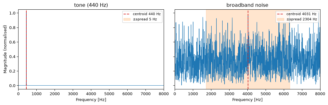
It is the standard correlate of perceived brightness. A muffled, boomy sound has a low centroid; a bright, buzzy, or hissy one has a high centroid. The spectral spread (also called bandwidth) is the magnitude-weighted standard deviation about that centroid, the second central moment:
It says how concentrated the energy is. A pure tone sits in one bin, so its spread is essentially zero; broadband noise smears across the band and has a large spread. Centroid and spread together are the mean and standard deviation of the spectrum read as a distribution over frequency.
Show the code
fs, L =16000.0, 4096freqs = np.fft.rfftfreq(L, 1/ fs)win = np.hanning(L)rng = np.random.default_rng(0)# a near-tone (440 Hz) and a broadband noise burstt = np.arange(L) / fstone = np.sin(2* np.pi *440* t)noise = rng.standard_normal(L)fig, axes = plt.subplots(1, 2, figsize=(11, 3.6), sharey=True)for ax, (x, name) inzip(axes, [(tone, 'tone (440 Hz)'), (noise, 'broadband noise')]): mag = np.abs(np.fft.rfft(x * win)) c =float(spectral_centroid(freqs, mag)) s =float(spectral_spread(freqs, mag)) ax.plot(freqs, mag / mag.max(), 'C0', lw=0.8) ax.axvline(c, color='C3', ls='--', label=f'centroid {c:.0f} Hz') ax.axvspan(max(c - s, 0), c + s, color='C1', alpha=0.2, label=f'±spread {s:.0f} Hz') ax.set_xlim(0, 8000); ax.set_xlabel('Frequency [Hz]'); ax.set_title(name) ax.legend(fontsize=8)axes[0].set_ylabel('Magnitude (normalised)')fig.tight_layout()plt.show()# the tone is brighter-pinned and far tighter than the noisec_tone =float(spectral_centroid(freqs, np.abs(np.fft.rfft(tone * win))))s_tone =float(spectral_spread(freqs, np.abs(np.fft.rfft(tone * win))))s_noise =float(spectral_spread(freqs, np.abs(np.fft.rfft(noise * win))))assertabs(c_tone -440) <30# centroid lands on the toneassert s_tone <100< s_noise # tone is tight, noise is wideprint(f"tone: centroid {c_tone:.0f} Hz, spread {s_tone:.0f} Hz")print(f"noise: spread {s_noise:.0f} Hz (>> the tone's)")
Figure 1: Centroid (the centre of mass, dashed) and spread (the standard deviation around it, shaded band) for a tonal sound and a broadband one. The tone pins the centroid at its frequency with almost no spread; the noise sits its centroid mid-band with a wide spread.
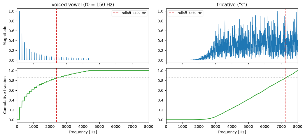
Where the centroid is a mean, the rolloff is a percentile of the spectrum. It is robust to a long, low tail of weak high-frequency energy: it tracks the upper edge of where the real energy lives. That makes it a good voiced-vs-unvoiced cue. A vowel keeps its energy low and rolls off early; a fricative like “s” pushes energy high and rolls off late.
Figure 2: Spectral rolloff (85%) for a voiced vowel and a fricative. The cumulative magnitude (lower panels) reaches 85% of its total far earlier for the vowel than for the hissy fricative, so the fricative’s rolloff sits much higher.
rolloff: vowel 2402 Hz vs fricative 7250 Hz
How it changes: flux
The four features so far describe a single frame. Spectral flux describes the change between consecutive frames: the Euclidean distance between successive magnitude spectra.
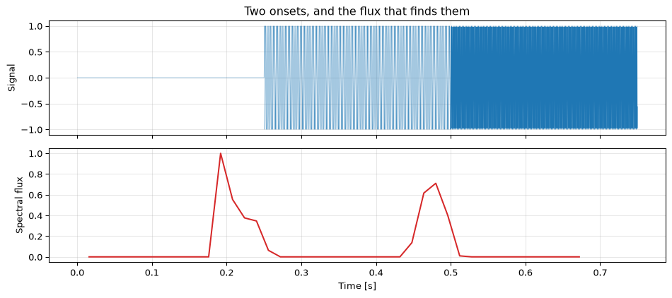
where \(m\) indexes frames and \(\tilde{X}_m\) is frame \(m\)’s magnitude spectrum after normalising to unit energy. With each frame normalised first, flux measures a change of spectral shape rather than of loudness. It sits near zero while a sound is steady and jumps at onsets and transients, where the spectrum is reorganising. The half-wave rectified version (keeping only bins that grew) is the classic note-onset detector; the symmetric form here is the general “how different is now from a moment ago” measure.
Show the code
def spectrogram_mag(x, nperseg, hop): w = np.hanning(nperseg) starts =range(0, len(x) - nperseg +1, hop)return np.stack([np.abs(np.fft.rfft(x[s:s + nperseg] * w)) for s in starts], axis=1)# silence -> 500 Hz -> 1500 Hz, each 0.25 sseg =int(0.25* fs)ts = np.arange(seg) / fssig = np.concatenate([np.zeros(seg), np.sin(2* np.pi *500* ts), np.sin(2* np.pi *1500* ts)])nperseg, hop =1024, 256M = spectrogram_mag(sig, nperseg, hop)flux = spectral_flux(M, normalize=True)frame_t = (np.arange(len(flux)) +1) * hop / fsfig, (a0, a1) = plt.subplots(2, 1, figsize=(10, 4.5), sharex=True)a0.plot(np.arange(len(sig)) / fs, sig, 'C0', lw=0.3)a0.set_ylabel('Signal'); a0.set_title('Two onsets, and the flux that finds them')a1.plot(frame_t, flux, 'C3'); a1.set_ylabel('Spectral flux'); a1.set_xlabel('Time [s]')for ax in (a0, a1): ax.grid(True, alpha=0.3)fig.tight_layout()plt.show()# flux spikes near each onset (~0.25, ~0.50 s; the long frame smears the exact# instant) and is tiny while a tone holds steadysteady = flux[(frame_t >0.30) & (frame_t <0.44)].mean() # mid first tone, clear of the next onset's smearonset1 = flux[(frame_t >0.15) & (frame_t <0.30)].max()onset2 = flux[(frame_t >0.43) & (frame_t <0.57)].max()assert onset1 >10* steady and onset2 >10* steadyprint(f"onset flux {onset1:.2f}, {onset2:.2f} vs steady flux {steady:.3f} (>10x)")
Figure 3: Spectral flux of a signal that steps from silence to one tone, then to a different tone. Flux spikes at each onset (the spectrum reorganises) and falls back to near zero while each tone holds steady.
onset flux 1.00, 0.71 vs steady flux 0.000 (>10x)
Tonal or noisy: flatness
The spectral flatness, or Wiener entropy, distinguishes a tonal spectrum from a noisy one. It is the ratio of the geometric mean of the power spectrum to its arithmetic mean:
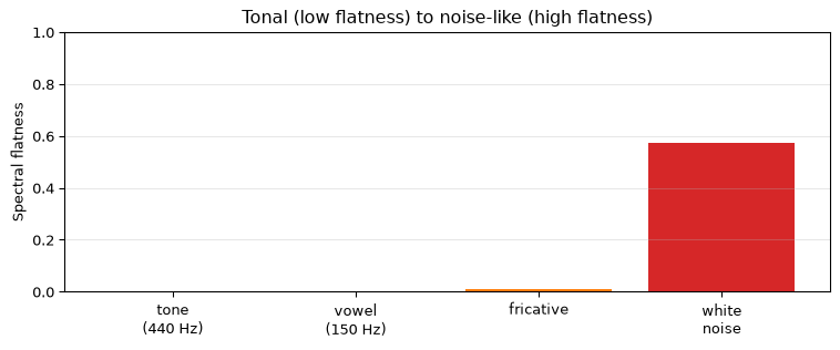
where \(K\) is the number of one-sided bins summed over. The geometric mean can never exceed the arithmetic mean, so flatness lives in \((0, 1]\). It equals 1 only when every bin has the same power, a perfectly flat (white) spectrum. A single dominant peak drags the geometric mean toward zero while barely moving the arithmetic mean, so a tone scores near zero. It is the cleanest single number for “is this voiced or is this noise”, and is often quoted in dB as \(10\log_{10}(\text{flatness})\).
Show the code
signals = {'tone\n(440 Hz)': tone, 'vowel\n(150 Hz)': vowel,'fricative': fric, 'white\nnoise': noise}flat = {name: float(spectral_flatness(np.abs(np.fft.rfft(x * win))))for name, x in signals.items()}fig, ax = plt.subplots(figsize=(8, 3.4))ax.bar(list(flat.keys()), list(flat.values()), color=['C0', 'C2', 'C1', 'C3'])ax.set_ylabel('Spectral flatness'); ax.set_ylim(0, 1)ax.set_title('Tonal (low flatness) to noise-like (high flatness)')ax.grid(True, axis='y', alpha=0.3)fig.tight_layout()plt.show()assert flat['tone\n(440 Hz)'] < flat['vowel\n(150 Hz)'] < flat['fricative'] < flat['white\nnoise']assert flat['white\nnoise'] >0.3# genuine noise is broadly flatprint({k: round(v, 3) for k, v in flat.items()})
Figure 4: Spectral flatness across a tone, a harmonic vowel, a fricative, and white noise. Flatness rises monotonically from the peaky tone to the flat noise floor, exactly the tonal-to-noisy axis it was built to measure.
Put one representative frame of each sound through all the per-frame features at once and the table reads like a fingerprint: each sound occupies a different corner of the feature space, which is exactly why a simple classifier can tell them apart from these numbers alone.
Show the code
from spectral_features import frame_featuresrows = []for name, x in [('tone (440 Hz)', tone), ('vowel (150 Hz)', vowel), ('fricative', fric), ('white noise', noise)]: mag = np.abs(np.fft.rfft(x * win)) f = frame_features(freqs, mag) rows.append((name, float(f['centroid']), float(f['spread']),float(f['rolloff']), float(f['flatness'])))print(f"{'sound':<16}{'centroid':>10}{'spread':>9}{'rolloff':>9}{'flatness':>10}")for name, c, s, r, fl in rows:print(f"{name:<16}{c:>9.0f}{s:>8.0f}{r:>8.0f}{fl:>9.3f}")# the qualitative orderings that make these features useful, pinned:cur = {name: vals for name, *vals in rows}assert cur['fricative'][0] > cur['vowel (150 Hz)'][0] # fricative is brighterassert cur['white noise'][1] > cur['tone (440 Hz)'][1] # noise is widerassert cur['fricative'][2] > cur['vowel (150 Hz)'][2] # fricative rolls off laterassert cur['white noise'][3] > cur['vowel (150 Hz)'][3] # noise is flatter
The centroid separates bright from dull, the spread concentrated from diffuse, the rolloff low-pitched from hissy, and the flatness tonal from noisy. None of them needs the phase, and all of them fall out of the same magnitude spectrum, so the marginal cost of computing all four is a few sums over bins you already have.
A trajectory, not a snapshot
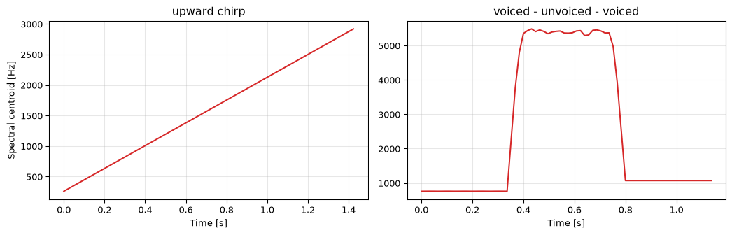
In practice you rarely keep a single frame. You run the STFT and get one feature value per frame, a trajectory that tracks how a sound evolves. The centroid trajectory of a swept tone climbs with the sweep; the centroid of a spoken phrase wobbles with each voiced and unvoiced segment.
Show the code
# a chirp 200 -> 3000 Hzdur =1.5tc = np.arange(int(fs * dur)) / fschirp = np.sin(2* np.pi * (200* tc + (3000-200) / (2* dur) * tc **2))# voiced - unvoiced - voicedsv =int(0.4* fs)tv = np.arange(sv) / fsv1 =sum((1.0/ k) * np.sin(2* np.pi *140* k * tv) for k inrange(1, 20))uv = sosfilt(sos, rng.standard_normal(sv))v2 =sum((1.0/ k) * np.sin(2* np.pi *200* k * tv) for k inrange(1, 20))utt = np.concatenate([v1, uv, v2])freqs_1024 = np.fft.rfftfreq(1024, 1/ fs) # this demo frames at 1024, not Lfig, axes = plt.subplots(1, 2, figsize=(11, 3.6))for ax, (x, name) inzip(axes, [(chirp, 'upward chirp'), (utt, 'voiced - unvoiced - voiced')]): Mx = spectrogram_mag(x, 1024, 256) c = spectral_centroid(freqs_1024, Mx) ft = np.arange(Mx.shape[1]) *256/ fs ax.plot(ft, c, 'C3'); ax.set_xlabel('Time [s]'); ax.set_title(name) ax.grid(True, alpha=0.3)axes[0].set_ylabel('Spectral centroid [Hz]')fig.tight_layout()plt.show()# the chirp centroid rises from start to end; the utterance centroid is highest mid (unvoiced)Mc = spectrogram_mag(chirp, 1024, 256)cc = spectral_centroid(np.fft.rfftfreq(1024, 1/ fs), Mc)assert cc[-1] > cc[0] +500# centroid climbs with the sweepMu = spectrogram_mag(utt, 1024, 256)cu = spectral_centroid(np.fft.rfftfreq(1024, 1/ fs), Mu)third =len(cu) //3assert cu[third:2* third].mean() > cu[:third].mean() # unvoiced middle is brighterprint("chirp centroid climbs; utterance centroid peaks in the unvoiced middle")
Figure 5: Centroid trajectory of an upward chirp (left) and of a voiced-unvoiced-voiced utterance (right). The chirp’s centroid tracks the instantaneous frequency almost linearly; the utterance’s centroid jumps up during the unvoiced middle segment, the same behaviour the voice-activity gate exploits.
chirp centroid climbs; utterance centroid peaks in the unvoiced middle
Going further
Deltas and aggregation. A single frame’s features are noisy. Real systems smooth them, take their first difference (the delta features, capturing rate of change), and aggregate over a window into means and variances. The same statistical-feature machinery is its own topic here.
More of the family. Beyond these five sit spectral skewness and kurtosis (the third and fourth moments of the same distribution), spectral crest, contrast, slope, and the perceptually-warped cousins. The most famous extension is the MFCC front end (a mel filterbank, a log, and a DCT turning the spectrum into a compact, decorrelated feature vector), its own topic here.
They feed classifiers, not decisions. On their own these features rarely make a clean decision; their power is as a low-dimensional input to a classifier or a gate. The pitch-detection VAD combines centroid and spread with energy and zero-crossing rate precisely because no one feature is enough.
Definition drift is real. Libraries disagree on the small print: magnitude versus power weighting, whether the DC bin is included, the rolloff percentage, whether flux is rectified. None of it is wrong, but cross-tool comparisons need the conventions matched. Peeters’ CUIDADO report (Peeters 2004) is the careful reference for the precise definitions.
References
Peeters, Geoffroy. 2004. “A Large Set of Audio Features for Sound Description (Similarity and Classification) in the CUIDADO Project.” IRCAM.
Tzanetakis, George, and Perry Cook. 2002. “Musical Genre Classification of Audio Signals.”IEEE Transactions on Speech and Audio Processing 10 (5): 293–302.
Source Code
---title: "Spectral Features"subtitle: "Describing the shape of a spectrum in a handful of numbers"description-meta: "Describing the shape of a spectrum in a handful of numbers: centroid, spread, flatness, rolloff and flux."bibliography: ../../references.bib---A spectrogram is a rich picture, but a classifier, a voice-activity gate, or a music-similarity search does not want a picture. It wants numbers: a few per frame that capture what the spectrum *looks like* without storing every bin. Is the energy low or high? Concentrated or spread out? Tonal or noise-like? Steady or changing?**Spectral features** answer exactly those questions. Each one collapses a frame's spectrum into a single descriptor, computed straight from the FFT bins the [STFT](../stft/index.qmd) already gave you. This page covers the five that turn up everywhere: the **centroid**, the **spread** (bandwidth), the **rolloff**, the **flux**, and the **flatness**. They are cheap, interpretable, and the workhorse front end of music information retrieval [@tzanetakis2002musical] and of the simplest viable speech and timbre classifiers.::: {.callout-note title="Prerequisites"}Part of the [feature extraction arc](../feature-extraction.qmd); the overview gives the reading order.These features live on top of the [Short-Time Fourier Transform](../stft/index.qmd): each is computed per frame from a one-sided magnitude spectrum. If the STFT is new, read that first. The [pitch-detection](../pitch-detection/index.qmd) page uses the centroid and spread as voice-activity cues; this page is the full family and their geometry.:::::: {.callout-tip title="Code"}The implementation is [`spectral_features.py`](spectral_features.py). Save [`test_spectral_features.py`](test_spectral_features.py) beside it and `pytest test_spectral_features.py` runs the checks on it.:::```{python}#| echo: falseimport numpy as npimport matplotlib.pyplot as pltfrom spectral_features import (spectral_centroid, spectral_spread, spectral_rolloff, spectral_flux, spectral_flatness)```## A convention first: magnitude or power?Every feature below weights the spectrum by something, and you have to say what. Two choices are common: the **magnitude** $|X[k]|$ of each bin, or its **power** $|X[k]|^2$. They are not the same descriptor; power leans harder on the loudest bins and so reports a slightly higher, tighter centre. Neither is wrong, but a page that mixes them silently is confusing, so this one fixes a convention and states it:- **Centroid, spread, rolloff** weight by **magnitude** $|X[k]|$. This is the common MIR convention (Tzanetakis & Cook, and librosa's default).- **Flatness** is defined on the **power** spectrum $|X[k]|^2$, where it is the classic Wiener entropy.If you prefer power weighting for the first three, pass `mag**2` in place of `mag`; the formulas are identical, only the weights change. (The [pitch-detection VAD](../pitch-detection/index.qmd#voice-activity-detection) uses the magnitude-weighted centroid, matching the convention here.)Throughout, $X[k]$ is the one-sided magnitude at bin $k$, and $f_k = k\,f_s/L$ is that bin's frequency. One more small print: the Python module here keeps the DC bin ($k=0$), while the embedded C on the [hardware page](embedded.qmd) skips it, since a residual DC offset sits at $f=0$, carries no perceptual information, and only drags the centroid down. For a windowed signal the difference is usually tiny, but it is the kind of convention that cross-tool comparisons need to match.## Where the energy sits: centroid and spreadThe **spectral centroid** is the magnitude-weighted mean frequency: the centre of mass of the spectrum.$$\mu = \frac{\sum_k f_k\,X[k]}{\sum_k X[k]}$$It is the standard correlate of perceived **brightness**. A muffled, boomy sound has a low centroid; a bright, buzzy, or hissy one has a high centroid. The **spectral spread** (also called bandwidth) is the magnitude-weighted standard deviation about that centroid, the second central moment:$$\sigma = \sqrt{\frac{\sum_k (f_k - \mu)^2\,X[k]}{\sum_k X[k]}}$$It says how *concentrated* the energy is. A pure tone sits in one bin, so its spread is essentially zero; broadband noise smears across the band and has a large spread. Centroid and spread together are the mean and standard deviation of the spectrum read as a distribution over frequency.```{python}#| label: fig-centroid-spread#| fig-cap: "Centroid (the centre of mass, dashed) and spread (the standard deviation around it, shaded band) for a tonal sound and a broadband one. The tone pins the centroid at its frequency with almost no spread; the noise sits its centroid mid-band with a wide spread."#| code-fold: truefs, L =16000.0, 4096freqs = np.fft.rfftfreq(L, 1/ fs)win = np.hanning(L)rng = np.random.default_rng(0)# a near-tone (440 Hz) and a broadband noise burstt = np.arange(L) / fstone = np.sin(2* np.pi *440* t)noise = rng.standard_normal(L)fig, axes = plt.subplots(1, 2, figsize=(11, 3.6), sharey=True)for ax, (x, name) inzip(axes, [(tone, 'tone (440 Hz)'), (noise, 'broadband noise')]): mag = np.abs(np.fft.rfft(x * win)) c =float(spectral_centroid(freqs, mag)) s =float(spectral_spread(freqs, mag)) ax.plot(freqs, mag / mag.max(), 'C0', lw=0.8) ax.axvline(c, color='C3', ls='--', label=f'centroid {c:.0f} Hz') ax.axvspan(max(c - s, 0), c + s, color='C1', alpha=0.2, label=f'±spread {s:.0f} Hz') ax.set_xlim(0, 8000); ax.set_xlabel('Frequency [Hz]'); ax.set_title(name) ax.legend(fontsize=8)axes[0].set_ylabel('Magnitude (normalised)')fig.tight_layout()plt.show()# the tone is brighter-pinned and far tighter than the noisec_tone =float(spectral_centroid(freqs, np.abs(np.fft.rfft(tone * win))))s_tone =float(spectral_spread(freqs, np.abs(np.fft.rfft(tone * win))))s_noise =float(spectral_spread(freqs, np.abs(np.fft.rfft(noise * win))))assertabs(c_tone -440) <30# centroid lands on the toneassert s_tone <100< s_noise # tone is tight, noise is wideprint(f"tone: centroid {c_tone:.0f} Hz, spread {s_tone:.0f} Hz")print(f"noise: spread {s_noise:.0f} Hz (>> the tone's)")```## Where it lies below: rolloffThe **spectral rolloff** is the frequency below which a fixed fraction (commonly 85%) of the spectral magnitude is found:$$f_R = \min\Bigl\{\,f_R : \sum_{f_k \le f_R} X[k] \;\ge\; 0.85 \sum_k X[k] \,\Bigr\}$$Where the centroid is a mean, the rolloff is a **percentile** of the spectrum. It is robust to a long, low tail of weak high-frequency energy: it tracks the upper edge of where the real energy lives. That makes it a good voiced-vs-unvoiced cue. A vowel keeps its energy low and rolls off early; a fricative like "s" pushes energy high and rolls off late.```{python}#| label: fig-rolloff#| fig-cap: "Spectral rolloff (85%) for a voiced vowel and a fricative. The cumulative magnitude (lower panels) reaches 85% of its total far earlier for the vowel than for the hissy fricative, so the fricative's rolloff sits much higher."#| code-fold: true# voiced vowel: a harmonic stack at f0 = 150 Hz, energy falling with harmonic numberf0 =150.0vowel =sum((1.0/ k) * np.sin(2* np.pi * f0 * k * t) for k inrange(1, 30))# fricative: high-pass-flavoured noise (energy above ~3 kHz)from scipy.signal import butter, sosfiltsos = butter(6, 3000, btype='high', fs=fs, output='sos')fric = sosfilt(sos, rng.standard_normal(L))fig, axes = plt.subplots(2, 2, figsize=(11, 5), sharex=True)for col, (x, name) inenumerate([(vowel, 'voiced vowel (f0 = 150 Hz)'), (fric, 'fricative ("s")')]): mag = np.abs(np.fft.rfft(x * win)) r =float(spectral_rolloff(freqs, mag, 0.85)) axes[0, col].plot(freqs, mag / mag.max(), 'C0', lw=0.8) axes[0, col].axvline(r, color='C3', ls='--', label=f'rolloff {r:.0f} Hz') axes[0, col].set_title(name); axes[0, col].legend(fontsize=8) cum = np.cumsum(mag) / mag.sum() axes[1, col].plot(freqs, cum, 'C2') axes[1, col].axhline(0.85, color='0.5', ls=':'); axes[1, col].axvline(r, color='C3', ls='--') axes[1, col].set_xlabel('Frequency [Hz]')axes[0, 0].set_ylabel('Magnitude'); axes[1, 0].set_ylabel('Cumulative fraction')axes[0, 0].set_xlim(0, 8000)fig.tight_layout()plt.show()r_vowel =float(spectral_rolloff(freqs, np.abs(np.fft.rfft(vowel * win)), 0.85))r_fric =float(spectral_rolloff(freqs, np.abs(np.fft.rfft(fric * win)), 0.85))assert r_fric > r_vowel # the fricative rolls off much laterprint(f"rolloff: vowel {r_vowel:.0f} Hz vs fricative {r_fric:.0f} Hz")```## How it changes: fluxThe four features so far describe a single frame. **Spectral flux** describes the *change* between consecutive frames: the Euclidean distance between successive magnitude spectra.$$F[m] = \sqrt{\sum_k \bigl(\tilde{X}_m[k] - \tilde{X}_{m-1}[k]\bigr)^2}$$where $m$ indexes frames and $\tilde{X}_m$ is frame $m$'s magnitude spectrum after normalising to unit energy. With each frame normalised first, flux measures a change of spectral *shape* rather than of loudness. It sits near zero while a sound is steady and jumps at **onsets** and transients, where the spectrum is reorganising. The half-wave rectified version (keeping only bins that grew) is the classic note-onset detector; the symmetric form here is the general "how different is now from a moment ago" measure.```{python}#| label: fig-flux#| fig-cap: "Spectral flux of a signal that steps from silence to one tone, then to a different tone. Flux spikes at each onset (the spectrum reorganises) and falls back to near zero while each tone holds steady."#| code-fold: truedef spectrogram_mag(x, nperseg, hop): w = np.hanning(nperseg) starts =range(0, len(x) - nperseg +1, hop)return np.stack([np.abs(np.fft.rfft(x[s:s + nperseg] * w)) for s in starts], axis=1)# silence -> 500 Hz -> 1500 Hz, each 0.25 sseg =int(0.25* fs)ts = np.arange(seg) / fssig = np.concatenate([np.zeros(seg), np.sin(2* np.pi *500* ts), np.sin(2* np.pi *1500* ts)])nperseg, hop =1024, 256M = spectrogram_mag(sig, nperseg, hop)flux = spectral_flux(M, normalize=True)frame_t = (np.arange(len(flux)) +1) * hop / fsfig, (a0, a1) = plt.subplots(2, 1, figsize=(10, 4.5), sharex=True)a0.plot(np.arange(len(sig)) / fs, sig, 'C0', lw=0.3)a0.set_ylabel('Signal'); a0.set_title('Two onsets, and the flux that finds them')a1.plot(frame_t, flux, 'C3'); a1.set_ylabel('Spectral flux'); a1.set_xlabel('Time [s]')for ax in (a0, a1): ax.grid(True, alpha=0.3)fig.tight_layout()plt.show()# flux spikes near each onset (~0.25, ~0.50 s; the long frame smears the exact# instant) and is tiny while a tone holds steadysteady = flux[(frame_t >0.30) & (frame_t <0.44)].mean() # mid first tone, clear of the next onset's smearonset1 = flux[(frame_t >0.15) & (frame_t <0.30)].max()onset2 = flux[(frame_t >0.43) & (frame_t <0.57)].max()assert onset1 >10* steady and onset2 >10* steadyprint(f"onset flux {onset1:.2f}, {onset2:.2f} vs steady flux {steady:.3f} (>10x)")```## Tonal or noisy: flatnessThe **spectral flatness**, or Wiener entropy, distinguishes a tonal spectrum from a noisy one. It is the ratio of the geometric mean of the power spectrum to its arithmetic mean:$$\text{flatness} = \frac{\Bigl(\prod_k |X[k]|^2\Bigr)^{1/K}}{\frac{1}{K}\sum_k |X[k]|^2}= \frac{\exp\!\bigl(\frac{1}{K}\sum_k \ln |X[k]|^2\bigr)}{\frac{1}{K}\sum_k |X[k]|^2}$$where $K$ is the number of one-sided bins summed over. The geometric mean can never exceed the arithmetic mean, so flatness lives in $(0, 1]$. It equals 1 only when every bin has the same power, a perfectly flat (white) spectrum. A single dominant peak drags the geometric mean toward zero while barely moving the arithmetic mean, so a tone scores near zero. It is the cleanest single number for "is this voiced or is this noise", and is often quoted in dB as $10\log_{10}(\text{flatness})$.```{python}#| label: fig-flatness#| fig-cap: "Spectral flatness across a tone, a harmonic vowel, a fricative, and white noise. Flatness rises monotonically from the peaky tone to the flat noise floor, exactly the tonal-to-noisy axis it was built to measure."#| code-fold: truesignals = {'tone\n(440 Hz)': tone, 'vowel\n(150 Hz)': vowel,'fricative': fric, 'white\nnoise': noise}flat = {name: float(spectral_flatness(np.abs(np.fft.rfft(x * win))))for name, x in signals.items()}fig, ax = plt.subplots(figsize=(8, 3.4))ax.bar(list(flat.keys()), list(flat.values()), color=['C0', 'C2', 'C1', 'C3'])ax.set_ylabel('Spectral flatness'); ax.set_ylim(0, 1)ax.set_title('Tonal (low flatness) to noise-like (high flatness)')ax.grid(True, axis='y', alpha=0.3)fig.tight_layout()plt.show()assert flat['tone\n(440 Hz)'] < flat['vowel\n(150 Hz)'] < flat['fricative'] < flat['white\nnoise']assert flat['white\nnoise'] >0.3# genuine noise is broadly flatprint({k: round(v, 3) for k, v in flat.items()})```## Reading the four sounds togetherPut one representative frame of each sound through all the per-frame features at once and the table reads like a fingerprint: each sound occupies a different corner of the feature space, which is exactly why a simple classifier can tell them apart from these numbers alone.```{python}#| label: tbl-fingerprint#| code-fold: truefrom spectral_features import frame_featuresrows = []for name, x in [('tone (440 Hz)', tone), ('vowel (150 Hz)', vowel), ('fricative', fric), ('white noise', noise)]: mag = np.abs(np.fft.rfft(x * win)) f = frame_features(freqs, mag) rows.append((name, float(f['centroid']), float(f['spread']),float(f['rolloff']), float(f['flatness'])))print(f"{'sound':<16}{'centroid':>10}{'spread':>9}{'rolloff':>9}{'flatness':>10}")for name, c, s, r, fl in rows:print(f"{name:<16}{c:>9.0f}{s:>8.0f}{r:>8.0f}{fl:>9.3f}")# the qualitative orderings that make these features useful, pinned:cur = {name: vals for name, *vals in rows}assert cur['fricative'][0] > cur['vowel (150 Hz)'][0] # fricative is brighterassert cur['white noise'][1] > cur['tone (440 Hz)'][1] # noise is widerassert cur['fricative'][2] > cur['vowel (150 Hz)'][2] # fricative rolls off laterassert cur['white noise'][3] > cur['vowel (150 Hz)'][3] # noise is flatter```The centroid separates bright from dull, the spread concentrated from diffuse, the rolloff low-pitched from hissy, and the flatness tonal from noisy. None of them needs the phase, and all of them fall out of the same magnitude spectrum, so the marginal cost of computing all four is a few sums over bins you already have.## A trajectory, not a snapshotIn practice you rarely keep a single frame. You run the STFT and get one feature value per frame, a **trajectory** that tracks how a sound evolves. The centroid trajectory of a swept tone climbs with the sweep; the centroid of a spoken phrase wobbles with each voiced and unvoiced segment.```{python}#| label: fig-trajectory#| fig-cap: "Centroid trajectory of an upward chirp (left) and of a voiced-unvoiced-voiced utterance (right). The chirp's centroid tracks the instantaneous frequency almost linearly; the utterance's centroid jumps up during the unvoiced middle segment, the same behaviour the voice-activity gate exploits."#| code-fold: true# a chirp 200 -> 3000 Hzdur =1.5tc = np.arange(int(fs * dur)) / fschirp = np.sin(2* np.pi * (200* tc + (3000-200) / (2* dur) * tc **2))# voiced - unvoiced - voicedsv =int(0.4* fs)tv = np.arange(sv) / fsv1 =sum((1.0/ k) * np.sin(2* np.pi *140* k * tv) for k inrange(1, 20))uv = sosfilt(sos, rng.standard_normal(sv))v2 =sum((1.0/ k) * np.sin(2* np.pi *200* k * tv) for k inrange(1, 20))utt = np.concatenate([v1, uv, v2])freqs_1024 = np.fft.rfftfreq(1024, 1/ fs) # this demo frames at 1024, not Lfig, axes = plt.subplots(1, 2, figsize=(11, 3.6))for ax, (x, name) inzip(axes, [(chirp, 'upward chirp'), (utt, 'voiced - unvoiced - voiced')]): Mx = spectrogram_mag(x, 1024, 256) c = spectral_centroid(freqs_1024, Mx) ft = np.arange(Mx.shape[1]) *256/ fs ax.plot(ft, c, 'C3'); ax.set_xlabel('Time [s]'); ax.set_title(name) ax.grid(True, alpha=0.3)axes[0].set_ylabel('Spectral centroid [Hz]')fig.tight_layout()plt.show()# the chirp centroid rises from start to end; the utterance centroid is highest mid (unvoiced)Mc = spectrogram_mag(chirp, 1024, 256)cc = spectral_centroid(np.fft.rfftfreq(1024, 1/ fs), Mc)assert cc[-1] > cc[0] +500# centroid climbs with the sweepMu = spectrogram_mag(utt, 1024, 256)cu = spectral_centroid(np.fft.rfftfreq(1024, 1/ fs), Mu)third =len(cu) //3assert cu[third:2* third].mean() > cu[:third].mean() # unvoiced middle is brighterprint("chirp centroid climbs; utterance centroid peaks in the unvoiced middle")```## Going further- **Deltas and aggregation.** A single frame's features are noisy. Real systems smooth them, take their first difference (the **delta** features, capturing rate of change), and aggregate over a window into means and variances. The same statistical-feature machinery is [its own topic here](../statistical-features/index.qmd).- **More of the family.** Beyond these five sit spectral **skewness** and **kurtosis** (the third and fourth moments of the same distribution), spectral **crest**, **contrast**, **slope**, and the perceptually-warped cousins. The most famous extension is the [MFCC front end](../mfcc/index.qmd) (a mel filterbank, a log, and a DCT turning the spectrum into a compact, decorrelated feature vector), its own topic here.- **They feed classifiers, not decisions.** On their own these features rarely make a clean decision; their power is as a low-dimensional input to a classifier or a gate. The [pitch-detection VAD](../pitch-detection/index.qmd#voice-activity-detection) combines centroid and spread with energy and zero-crossing rate precisely because no one feature is enough.- **Definition drift is real.** Libraries disagree on the small print: magnitude versus power weighting, whether the DC bin is included, the rolloff percentage, whether flux is rectified. None of it is wrong, but cross-tool comparisons need the conventions matched. Peeters' CUIDADO report [@peeters2004large] is the careful reference for the precise definitions.## References::: {#refs}:::