Decimation, interpolation, and sample rate conversion
Nature’s multirate system
The human retina is a biological multirate system: the fovea (central 2 degrees) samples at extremely high spatial resolution, while the periphery progressively decimates, trading resolution for wider coverage (Curcio et al. 1990). This is the same bandwidth-efficiency trade-off that drives digital multirate processing: sample densely where detail matters, decimate where it doesn’t.
Sampling a signal at 1 MHz when you only need 10 kHz of bandwidth wastes storage, bus bandwidth, and processing cycles. Conversely, converting audio between 44.1 kHz and 48 kHz (two sample rates that exist because the CD and professional audio industries could not agree on a standard) requires changing the rate by a non-integer factor. Multirate signal processing provides the tools to move between sample rates efficiently and correctly. For embedded implementations — CIC filters, CMSIS-DSP polyphase decimation, and two-stage pipelines on STM32F4 and ESP32-S3 — see Multirate on Hardware.
The applications are everywhere. Sigma-delta ADCs oversample at many times the Nyquist rate, then decimate digitally to achieve high resolution with simple analog front-ends. Software-defined radios digitise wide bands at high rates, then decimate to isolate narrow channels. Audio equipment routinely converts between 44.1, 48, 88.2, 96, and 192 kHz. In all these cases, the core operations are the same: decimation, interpolation, and the filters that make them work.
Prerequisites
This topic assumes familiarity with the frequency domain (particularly spectral effects of sampling) and filter design (anti-aliasing and FIR design).
Decimation (downsampling)
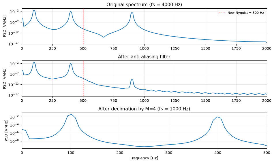
Decimation reduces the sample rate by an integer factor \(M\): keep every \(M\)-th sample, discard the rest. But you cannot simply throw away samples. That would alias any spectral content above the new Nyquist frequency \(f_s / (2M)\) back into the baseband.
The correct procedure is:
Anti-aliasing filter: a lowpass filter with cutoff \(f_s / (2M)\)
Downsample by \(M\): keep every \(M\)-th sample
The output sample rate is \(f_s / M\), and the anti-aliasing filter ensures that no aliased components fold into the output band.
Mathematically, if \(x[n]\) is filtered to produce \(x_f[n]\), the decimated output is:
\[y[m] = x_f[mM]\]
In the frequency domain, downsampling by \(M\) causes spectral folding. The DTFT of the decimated signal is:
The \(M\) shifted copies of the spectrum overlap; without the anti-aliasing filter, they alias destructively.
import numpy as npimport matplotlib.pyplot as pltfrom scipy import signal as sig# Create a test signal: sum of sinusoids at 100, 400, and 900 Hzfs =4000N =2000t = np.arange(N) / fsx = np.sin(2* np.pi *100* t) +0.5* np.sin(2* np.pi *400* t) +0.3* np.sin(2* np.pi *900* t)M =4fs_new = fs // M# Anti-aliasing filter: lowpass at fs/(2M) = 500 Hzb_aa = sig.firwin(65, 1.0/ M)x_filtered = sig.lfilter(b_aa, 1.0, x)# Decimatex_dec = x_filtered[::M]fig, axes = plt.subplots(3, 1, figsize=(10, 6))# Original spectrumf_orig, Pxx_orig = sig.welch(x, fs, nperseg=512)axes[0].semilogy(f_orig, Pxx_orig)axes[0].set_title(f'Original spectrum (fs = {fs} Hz)')axes[0].set_ylabel('PSD [V²/Hz]')axes[0].axvline(fs_new /2, color='r', linestyle='--', linewidth=1, label=f'New Nyquist = {fs_new//2} Hz')axes[0].legend(fontsize=8)# After anti-aliasing filterf_filt, Pxx_filt = sig.welch(x_filtered, fs, nperseg=512)axes[1].semilogy(f_filt, Pxx_filt)axes[1].set_title('After anti-aliasing filter')axes[1].set_ylabel('PSD [V²/Hz]')axes[1].axvline(fs_new /2, color='r', linestyle='--', linewidth=1)# After decimationf_dec, Pxx_dec = sig.welch(x_dec, fs_new, nperseg=128)axes[2].semilogy(f_dec, Pxx_dec)axes[2].set_title(f'After decimation by M={M} (fs = {fs_new} Hz)')axes[2].set_ylabel('PSD [V²/Hz]')axes[2].set_xlabel('Frequency [Hz]')for ax in axes: ax.set_xlim(0, fs /2) ax.grid(True, alpha=0.3)axes[2].set_xlim(0, fs_new /2)fig.tight_layout()plt.show()
Figure 1: Decimation by M=4. Top: original signal spectrum. Middle: after anti-aliasing filter. Bottom: after downsampling, the spectrum is stretched by M, filling the new Nyquist band.
SciPy provides scipy.signal.decimate, which handles the anti-aliasing filter and downsampling in one call. By default it uses a Chebyshev Type I IIR filter, though FIR is often preferable for multirate work (the ftype='fir' option).
Interpolation (upsampling)
Interpolation increases the sample rate by an integer factor \(L\). The procedure mirrors decimation:
Upsample by \(L\): insert \(L-1\) zeros between each sample
Anti-imaging filter: a lowpass filter with cutoff \(f_s / 2\) (the original Nyquist, equivalently \(f_{s,\text{out}}/(2L)\)) and gain \(L\)
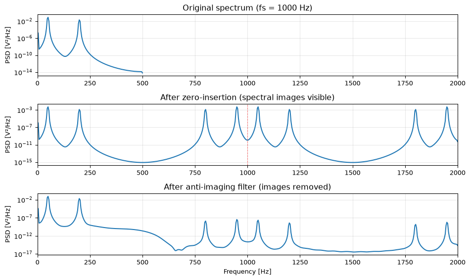
The zero-insertion step creates \(L-1\) spectral images (copies of the baseband spectrum centred at multiples of the original sample rate). The anti-imaging filter removes these images, leaving only the baseband.
The upsampled signal before filtering is:
\[x_u[n] = \begin{cases} x[n/L] & \text{if } n \text{ is a multiple of } L \\ 0 & \text{otherwise} \end{cases}\]
Its spectrum contains \(L\) copies of the original:
\[X_u(e^{j\omega}) = X(e^{j\omega L})\]
The anti-imaging filter passes only the copy centred at DC and applies a gain of \(L\) to restore the correct amplitude.
# Original signal at low ratefs_low =1000N_low =500t_low = np.arange(N_low) / fs_lowx_low = np.sin(2* np.pi *50* t_low) +0.5* np.sin(2* np.pi *200* t_low)L =4fs_high = fs_low * L# Zero insertionx_up = np.zeros(N_low * L)x_up[::L] = x_low# Anti-imaging filter (gain = L to compensate for zero insertion)b_ai = sig.firwin(65, 1.0/ L) * Lx_interp = sig.lfilter(b_ai, 1.0, x_up)fig, axes = plt.subplots(3, 1, figsize=(10, 6))# Original spectrumf1, P1 = sig.welch(x_low, fs_low, nperseg=256)axes[0].semilogy(f1, P1)axes[0].set_title(f'Original spectrum (fs = {fs_low} Hz)')axes[0].set_ylabel('PSD [V²/Hz]')# After zero insertion — show full Nyquist band of the upsampled ratef2, P2 = sig.welch(x_up, fs_high, nperseg=1024)axes[1].semilogy(f2, P2)axes[1].set_title(f'After zero-insertion (spectral images visible)')axes[1].set_ylabel('PSD [V²/Hz]')for k inrange(1, L): axes[1].axvline(k * fs_low, color='r', linestyle='--', linewidth=0.8, alpha=0.5)# After anti-imaging filterf3, P3 = sig.welch(x_interp, fs_high, nperseg=1024)axes[2].semilogy(f3, P3)axes[2].set_title('After anti-imaging filter (images removed)')axes[2].set_ylabel('PSD [V²/Hz]')axes[2].set_xlabel('Frequency [Hz]')for ax in axes: ax.set_xlim(0, fs_high /2) ax.grid(True, alpha=0.3)fig.tight_layout()plt.show()
Figure 2: Interpolation by L=4. Top: original signal. Middle: after zero-insertion, spectral images appear at multiples of the original fs. Bottom: after anti-imaging filter removes the images.
Rational rate conversion
What if you need to convert from 44.1 kHz to 48 kHz? The ratio is \(48000/44100 = 160/147\): neither a pure integer upsample nor downsample. The solution is to interpolate by \(L\) then decimate by \(M\), where \(L/M\) equals the desired rate ratio:
The key insight is that the interpolation and decimation filters can be combined into a single filter. Both require a lowpass: the interpolation filter has cutoff \(\pi/L\) and the decimation filter has cutoff \(\pi/M\). The combined filter uses the more restrictive of the two:
In practice, scipy.signal.resample_poly(x, L, M) does this efficiently. It designs the combined anti-aliasing/anti-imaging FIR filter and uses polyphase decomposition internally so that computation is proportional to the output length, not the high intermediate rate \(L \cdot f_s\).
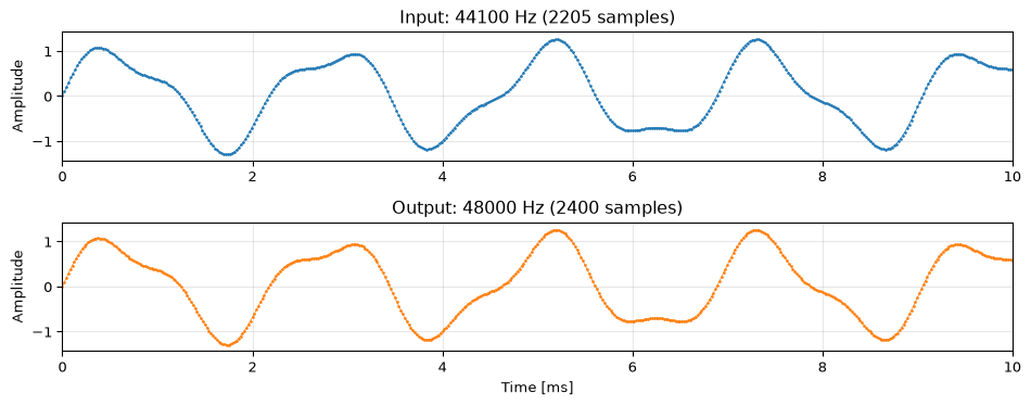
# Simulate a short audio segment at 44.1 kHzfs_in =44100duration =0.05# 50 mst_in = np.arange(int(fs_in * duration)) / fs_inx_in = np.sin(2* np.pi *440* t_in) +0.3* np.sin(2* np.pi *1000* t_in)# Rational SRCL, M =160, 147fs_out = fs_in * L // M # 48000x_out = sig.resample_poly(x_in, L, M)t_out = np.arange(len(x_out)) / fs_outfig, axes = plt.subplots(2, 1, figsize=(10, 4))axes[0].plot(t_in *1000, x_in, '.-', markersize=2, linewidth=0.5)axes[0].set_title(f'Input: {fs_in} Hz ({len(x_in)} samples)')axes[0].set_ylabel('Amplitude')axes[1].plot(t_out *1000, x_out, '.-', markersize=2, linewidth=0.5, color='C1')axes[1].set_title(f'Output: {fs_out} Hz ({len(x_out)} samples)')axes[1].set_ylabel('Amplitude')axes[1].set_xlabel('Time [ms]')for ax in axes: ax.set_xlim(0, 10) # Show first 10 ms ax.grid(True, alpha=0.3)fig.tight_layout()plt.show()
Figure 3: Rational sample rate conversion: 44.1 kHz to 48 kHz using L=160, M=147. The signal content is preserved while the sample rate changes.
The 44.1 vs 48 kHz problem
The 44.1/48 kHz conversion is the classic multirate problem in audio. 44,100 Hz was chosen for the CD standard (derived from video line rates), while 48,000 Hz became the professional audio and broadcast standard. Every time audio moves between consumer and professional domains (DAWs, streaming services, broadcast chains) this conversion happens. The ratio 160/147 is not close to any small integer, so the polyphase filter is long. Getting this conversion transparent (no audible artifacts) is a solved problem, but it took decades of engineering.
A related experiment: play a 44.1 kHz recording at 48 kHz without resampling. Every sample is interpreted as occurring \(48000/44100 \approx 1.088\) times too fast, so pitch shifts up by about 1.5 semitones and duration shrinks by 8.1% (\(1 - 44100/48000\)). The Beethoven demo in DSP2 course material uses this to dramatic effect: a symphony in the wrong key.
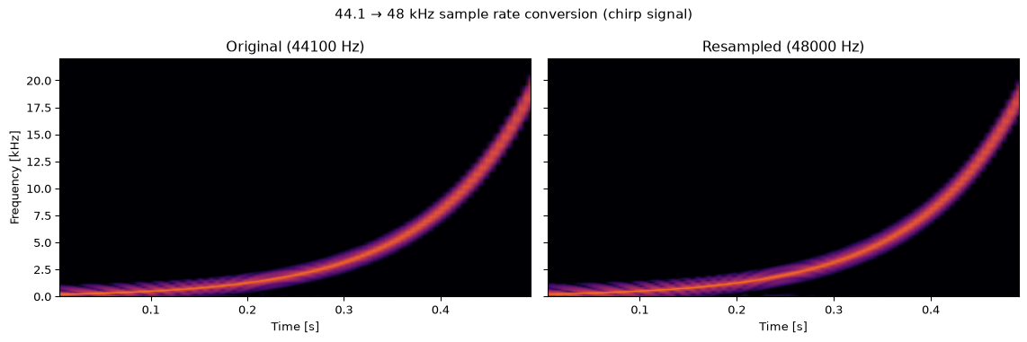
The following demo generates a chirp signal, resamples it from 44.1 to 48 kHz using resample_poly, and compares the spectrograms to verify that spectral content is preserved without aliasing artifacts.
import numpy as npimport matplotlib.pyplot as pltfrom scipy import signal as sig# Generate a chirp at 44.1 kHz: sweep from 200 Hz to 20 kHz over 0.5 sfs_441 =44100duration =0.5t_441 = np.arange(int(fs_441 * duration)) / fs_441chirp = sig.chirp(t_441, f0=200, f1=20000, t1=duration, method='logarithmic')# Resample to 48 kHzL, M =160, 147fs_48 =48000chirp_48 = sig.resample_poly(chirp, L, M)t_48 = np.arange(len(chirp_48)) / fs_48fig, axes = plt.subplots(1, 2, figsize=(12, 4), sharey=True)nperseg =512for ax, x, fs_val, title in [ (axes[0], chirp, fs_441, f'Original ({fs_441} Hz)'), (axes[1], chirp_48, fs_48, f'Resampled ({fs_48} Hz)')]: f, t_spec, Sxx = sig.spectrogram(x, fs_val, nperseg=nperseg, noverlap=nperseg//2) ax.pcolormesh(t_spec, f /1000, 10* np.log10(Sxx +1e-12), shading='gouraud', cmap='inferno', vmin=-80, vmax=0) ax.set_xlabel('Time [s]') ax.set_title(title) ax.set_ylim(0, 22)axes[0].set_ylabel('Frequency [kHz]')fig.suptitle('44.1 → 48 kHz sample rate conversion (chirp signal)', fontsize=11)fig.tight_layout()plt.show()
Figure 4: Resampling a chirp from 44.1 kHz to 48 kHz. The spectrogram shows the frequency sweep is preserved cleanly, no aliasing, no spectral artifacts.
Polyphase decomposition
The naive approach to interpolation by \(L\) is expensive: insert zeros, then filter at the high rate \(L \cdot f_s\). But \(L-1\) out of every \(L\) input samples to the filter are zero, so most of the multiply-accumulate operations produce nothing. Polyphase decomposition eliminates this waste (Crochiere and Rabiner 1983).
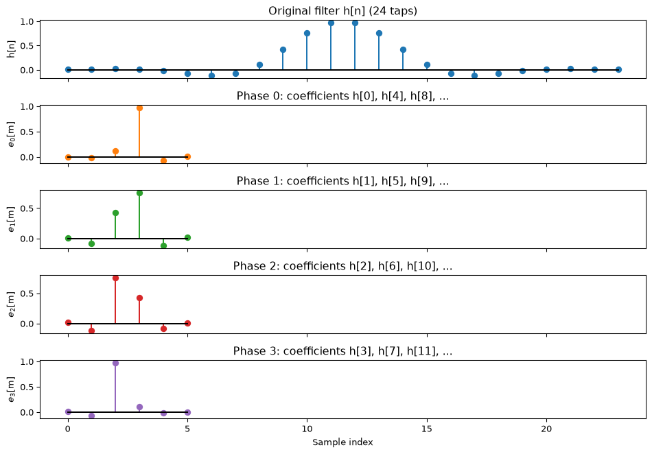
The idea is to split the filter \(H(z)\) of length \(N\) into \(L\) subfilters (phases), each of length \(N/L\):
\[H(z) = \sum_{k=0}^{L-1} z^{-k} E_k(z^L)\]
where the \(k\)-th polyphase component contains every \(L\)-th coefficient:
Each subfilter \(E_k\) operates at the low sample rate. The outputs are interleaved to form the high-rate signal. The computational cost drops by a factor of \(L\) compared to the direct approach.
For decimation, the same principle applies in reverse: the input is split into \(M\) polyphase components (a commutator distributing successive input samples to \(M\) branches), each branch is filtered at the low rate, and the outputs are summed.
Figure 5: Polyphase decomposition of a 24-tap FIR filter into L=4 subfilters. Each subfilter operates at the low sample rate, reducing computation by a factor of L.
Tip
SciPy’s resample_poly uses polyphase decomposition internally. You get the efficiency gains without implementing the decomposition yourself. For custom implementations (e.g., on embedded hardware), the polyphase structure maps naturally to a round-robin of short FIR filters.
Multi-stage decimation
Decimating by a large factor \(M\) in a single stage requires a very sharp anti-aliasing filter: the transition band must be narrow relative to the output bandwidth. For \(M = 100\) with \(f_s = 100\) kHz, the anti-aliasing filter needs a cutoff at 500 Hz with a transition band of a few hundred Hz at most. This requires thousands of taps.
Multi-stage decimation breaks the operation into cascaded stages with smaller decimation factors. For \(M = 100\):
Single stage: \(\div 100\) (very sharp filter, very expensive)
Two stages: \(\div 10 \to \div 10\) (two moderate filters, much cheaper)
Why is this more efficient? Each subsequent stage operates at a lower sample rate, so its filter runs fewer multiply-accumulates per second. And the transition band requirements are relaxed: each stage only needs to prevent aliasing down to its own output Nyquist frequency, not the final one.
The total number of multiplications per output sample for a cascade is typically much less than for a single stage. The optimal number of stages and the factor split depend on the specific \(M\) and the required stopband attenuation, and finding the optimal decomposition is itself an interesting design problem.
CIC filters
The Cascaded Integrator-Comb (CIC) filter is a special case of multi-stage decimation that uses no multiplications at all. A CIC of order \(K\) decimating by \(M\) is:
This factorises into a comb filter \((1 - z^{-M})\) operating at the high rate and an integrator \(1/(1 - z^{-1})\) operating at the low rate, both requiring only additions and subtractions.
CIC filters are ubiquitous in sigma-delta ADCs and FPGA-based SDR front-ends, where they handle the first stage of decimation from very high oversampling rates (Hogenauer 1981). Their frequency response is a sinc-like shape with nulls at multiples of \(f_{s,\text{in}}/M\) (where \(f_{s,\text{in}}\) is the input sample rate), which is adequate for a first-stage decimation but typically needs a compensation filter (a short FIR) afterwards to flatten the passband.
Open questions
Arbitrary and irrational rate conversion. Rational conversion with \(L/M\) only works when the rate ratio is rational. For truly arbitrary conversion (e.g., synchronising to a clock that drifts continuously), polynomial interpolation (Farrow structure) or time-varying fractional delay filters are needed. These are well understood theoretically but tricky to implement with low latency.
Time-varying rates. In adaptive sample rate conversion (for example, synchronising an audio stream to a clock recovered from a network) the conversion ratio changes continuously. The polyphase filter coefficients must be interpolated in real time. This is standard practice in professional audio but rarely covered in textbooks.
Streaming with block processing. Most multirate descriptions assume infinite signals. In practice, signals arrive in blocks, and filter states must be carried across block boundaries. Getting the edge effects right, especially for multi-stage cascades, is a common source of bugs in real-time implementations.
Non-uniform sampling. What if the input is not uniformly sampled? Reconstruction and rate conversion from non-uniform samples connects to compressed sensing and is an active research area.
References
Crochiere, Ronald E., and Lawrence R. Rabiner. 1983. Multirate Digital Signal Processing. Prentice-Hall.
Curcio, Christine A., Kenneth R. Sloan, Robert E. Kalina, and Anita E. Hendrickson. 1990. “Human Photoreceptor Topography.”Journal of Comparative Neurology 292 (4): 497–523.
Hogenauer, Eugene B. 1981. “An Economical Class of Digital Filters for Decimation and Interpolation.”IEEE Transactions on Acoustics, Speech, and Signal Processing 29 (2): 155–62.
Source Code
---title: "Multirate Systems"subtitle: "Decimation, interpolation, and sample rate conversion"---::: {.callout-tip title="Nature's multirate system" appearance="simple"}The human retina is a biological multirate system: the fovea (central 2 degrees) samples at extremely high spatial resolution, while the periphery progressively decimates, trading resolution for wider coverage [@curcio1990human]. This is the same bandwidth-efficiency trade-off that drives digital multirate processing: sample densely where detail matters, decimate where it doesn't.:::Sampling a signal at 1 MHz when you only need 10 kHz of bandwidth wastes storage, bus bandwidth, and processing cycles. Conversely, converting audio between 44.1 kHz and 48 kHz (two sample rates that exist because the CD and professional audio industries could not agree on a standard) requires changing the rate by a non-integer factor. **Multirate signal processing** provides the tools to move between sample rates efficiently and correctly. For embedded implementations --- CIC filters, CMSIS-DSP polyphase decimation, and two-stage pipelines on STM32F4 and ESP32-S3 --- see [Multirate on Hardware](embedded.qmd).The applications are everywhere. Sigma-delta ADCs oversample at many times the Nyquist rate, then decimate digitally to achieve high resolution with simple analog front-ends. Software-defined radios digitise wide bands at high rates, then decimate to isolate narrow channels. Audio equipment routinely converts between 44.1, 48, 88.2, 96, and 192 kHz. In all these cases, the core operations are the same: decimation, interpolation, and the filters that make them work.::: {.callout-note title="Prerequisites"}This topic assumes familiarity with the [frequency domain](../../basics/05-frequency-domain.qmd) (particularly spectral effects of sampling) and [filter design](../../basics/06-filter-design.qmd) (anti-aliasing and FIR design).:::---## Decimation (downsampling)**Decimation** reduces the sample rate by an integer factor $M$: keep every $M$-th sample, discard the rest. But you cannot simply throw away samples. That would alias any spectral content above the new Nyquist frequency $f_s / (2M)$ back into the baseband.The correct procedure is:1. **Anti-aliasing filter**: a lowpass filter with cutoff $f_s / (2M)$2. **Downsample by $M$**: keep every $M$-th sampleThe output sample rate is $f_s / M$, and the anti-aliasing filter ensures that no aliased components fold into the output band.Mathematically, if $x[n]$ is filtered to produce $x_f[n]$, the decimated output is:$$y[m] = x_f[mM]$$In the frequency domain, downsampling by $M$ causes spectral folding. The DTFT of the decimated signal is:$$Y(e^{j\omega}) = \frac{1}{M} \sum_{k=0}^{M-1} X_f\!\left(e^{\,j\frac{\omega - 2\pi k}{M}}\right)$$The $M$ shifted copies of the spectrum overlap; without the anti-aliasing filter, they alias destructively.```{python}#| label: fig-decimation#| fig-cap: "Decimation by M=4. Top: original signal spectrum. Middle: after anti-aliasing filter. Bottom: after downsampling, the spectrum is stretched by M, filling the new Nyquist band."import numpy as npimport matplotlib.pyplot as pltfrom scipy import signal as sig# Create a test signal: sum of sinusoids at 100, 400, and 900 Hzfs =4000N =2000t = np.arange(N) / fsx = np.sin(2* np.pi *100* t) +0.5* np.sin(2* np.pi *400* t) +0.3* np.sin(2* np.pi *900* t)M =4fs_new = fs // M# Anti-aliasing filter: lowpass at fs/(2M) = 500 Hzb_aa = sig.firwin(65, 1.0/ M)x_filtered = sig.lfilter(b_aa, 1.0, x)# Decimatex_dec = x_filtered[::M]fig, axes = plt.subplots(3, 1, figsize=(10, 6))# Original spectrumf_orig, Pxx_orig = sig.welch(x, fs, nperseg=512)axes[0].semilogy(f_orig, Pxx_orig)axes[0].set_title(f'Original spectrum (fs = {fs} Hz)')axes[0].set_ylabel('PSD [V²/Hz]')axes[0].axvline(fs_new /2, color='r', linestyle='--', linewidth=1, label=f'New Nyquist = {fs_new//2} Hz')axes[0].legend(fontsize=8)# After anti-aliasing filterf_filt, Pxx_filt = sig.welch(x_filtered, fs, nperseg=512)axes[1].semilogy(f_filt, Pxx_filt)axes[1].set_title('After anti-aliasing filter')axes[1].set_ylabel('PSD [V²/Hz]')axes[1].axvline(fs_new /2, color='r', linestyle='--', linewidth=1)# After decimationf_dec, Pxx_dec = sig.welch(x_dec, fs_new, nperseg=128)axes[2].semilogy(f_dec, Pxx_dec)axes[2].set_title(f'After decimation by M={M} (fs = {fs_new} Hz)')axes[2].set_ylabel('PSD [V²/Hz]')axes[2].set_xlabel('Frequency [Hz]')for ax in axes: ax.set_xlim(0, fs /2) ax.grid(True, alpha=0.3)axes[2].set_xlim(0, fs_new /2)fig.tight_layout()plt.show()```SciPy provides `scipy.signal.decimate`, which handles the anti-aliasing filter and downsampling in one call. By default it uses a Chebyshev Type I IIR filter, though FIR is often preferable for multirate work (the `ftype='fir'` option).---## Interpolation (upsampling)**Interpolation** increases the sample rate by an integer factor $L$. The procedure mirrors decimation:1. **Upsample by $L$**: insert $L-1$ zeros between each sample2. **Anti-imaging filter**: a lowpass filter with cutoff $f_s / 2$ (the original Nyquist, equivalently $f_{s,\text{out}}/(2L)$) and gain $L$The zero-insertion step creates $L-1$ spectral images (copies of the baseband spectrum centred at multiples of the original sample rate). The anti-imaging filter removes these images, leaving only the baseband.The upsampled signal before filtering is:$$x_u[n] = \begin{cases} x[n/L] & \text{if } n \text{ is a multiple of } L \\ 0 & \text{otherwise} \end{cases}$$Its spectrum contains $L$ copies of the original:$$X_u(e^{j\omega}) = X(e^{j\omega L})$$The anti-imaging filter passes only the copy centred at DC and applies a gain of $L$ to restore the correct amplitude.```{python}#| label: fig-interpolation#| fig-cap: "Interpolation by L=4. Top: original signal. Middle: after zero-insertion, spectral images appear at multiples of the original fs. Bottom: after anti-imaging filter removes the images."# Original signal at low ratefs_low =1000N_low =500t_low = np.arange(N_low) / fs_lowx_low = np.sin(2* np.pi *50* t_low) +0.5* np.sin(2* np.pi *200* t_low)L =4fs_high = fs_low * L# Zero insertionx_up = np.zeros(N_low * L)x_up[::L] = x_low# Anti-imaging filter (gain = L to compensate for zero insertion)b_ai = sig.firwin(65, 1.0/ L) * Lx_interp = sig.lfilter(b_ai, 1.0, x_up)fig, axes = plt.subplots(3, 1, figsize=(10, 6))# Original spectrumf1, P1 = sig.welch(x_low, fs_low, nperseg=256)axes[0].semilogy(f1, P1)axes[0].set_title(f'Original spectrum (fs = {fs_low} Hz)')axes[0].set_ylabel('PSD [V²/Hz]')# After zero insertion — show full Nyquist band of the upsampled ratef2, P2 = sig.welch(x_up, fs_high, nperseg=1024)axes[1].semilogy(f2, P2)axes[1].set_title(f'After zero-insertion (spectral images visible)')axes[1].set_ylabel('PSD [V²/Hz]')for k inrange(1, L): axes[1].axvline(k * fs_low, color='r', linestyle='--', linewidth=0.8, alpha=0.5)# After anti-imaging filterf3, P3 = sig.welch(x_interp, fs_high, nperseg=1024)axes[2].semilogy(f3, P3)axes[2].set_title('After anti-imaging filter (images removed)')axes[2].set_ylabel('PSD [V²/Hz]')axes[2].set_xlabel('Frequency [Hz]')for ax in axes: ax.set_xlim(0, fs_high /2) ax.grid(True, alpha=0.3)fig.tight_layout()plt.show()```---## Rational rate conversionWhat if you need to convert from 44.1 kHz to 48 kHz? The ratio is $48000/44100 = 160/147$: neither a pure integer upsample nor downsample. The solution is to **interpolate by $L$ then decimate by $M$**, where $L/M$ equals the desired rate ratio:$$f_{s,\text{out}} = f_{s,\text{in}} \cdot \frac{L}{M}$$For 44.1 to 48 kHz: $L = 160$, $M = 147$.The key insight is that the interpolation and decimation filters can be **combined into a single filter**. Both require a lowpass: the interpolation filter has cutoff $\pi/L$ and the decimation filter has cutoff $\pi/M$. The combined filter uses the more restrictive of the two:$$\omega_c = \min\!\left(\frac{\pi}{L}, \frac{\pi}{M}\right) = \frac{\pi}{\max(L, M)}$$In practice, `scipy.signal.resample_poly(x, L, M)` does this efficiently. It designs the combined anti-aliasing/anti-imaging FIR filter and uses polyphase decomposition internally so that computation is proportional to the output length, not the high intermediate rate $L \cdot f_s$.```{python}#| label: fig-src#| fig-cap: "Rational sample rate conversion: 44.1 kHz to 48 kHz using L=160, M=147. The signal content is preserved while the sample rate changes."# Simulate a short audio segment at 44.1 kHzfs_in =44100duration =0.05# 50 mst_in = np.arange(int(fs_in * duration)) / fs_inx_in = np.sin(2* np.pi *440* t_in) +0.3* np.sin(2* np.pi *1000* t_in)# Rational SRCL, M =160, 147fs_out = fs_in * L // M # 48000x_out = sig.resample_poly(x_in, L, M)t_out = np.arange(len(x_out)) / fs_outfig, axes = plt.subplots(2, 1, figsize=(10, 4))axes[0].plot(t_in *1000, x_in, '.-', markersize=2, linewidth=0.5)axes[0].set_title(f'Input: {fs_in} Hz ({len(x_in)} samples)')axes[0].set_ylabel('Amplitude')axes[1].plot(t_out *1000, x_out, '.-', markersize=2, linewidth=0.5, color='C1')axes[1].set_title(f'Output: {fs_out} Hz ({len(x_out)} samples)')axes[1].set_ylabel('Amplitude')axes[1].set_xlabel('Time [ms]')for ax in axes: ax.set_xlim(0, 10) # Show first 10 ms ax.grid(True, alpha=0.3)fig.tight_layout()plt.show()```::: {.callout-note title="The 44.1 vs 48 kHz problem"}The 44.1/48 kHz conversion is *the* classic multirate problem in audio. 44,100 Hz was chosen for the CD standard (derived from video line rates), while 48,000 Hz became the professional audio and broadcast standard. Every time audio moves between consumer and professional domains (DAWs, streaming services, broadcast chains) this conversion happens. The ratio 160/147 is not close to any small integer, so the polyphase filter is long. Getting this conversion transparent (no audible artifacts) is a solved problem, but it took decades of engineering.A related experiment: play a 44.1 kHz recording at 48 kHz without resampling. Every sample is interpreted as occurring $48000/44100 \approx 1.088$ times too fast, so pitch shifts up by about 1.5 semitones and duration shrinks by 8.1% ($1 - 44100/48000$). The Beethoven demo in DSP2 course material uses this to dramatic effect: a symphony in the wrong key.:::The following demo generates a chirp signal, resamples it from 44.1 to 48 kHz using `resample_poly`, and compares the spectrograms to verify that spectral content is preserved without aliasing artifacts.```{python}#| label: fig-audio-resample#| fig-cap: "Resampling a chirp from 44.1 kHz to 48 kHz. The spectrogram shows the frequency sweep is preserved cleanly, no aliasing, no spectral artifacts."import numpy as npimport matplotlib.pyplot as pltfrom scipy import signal as sig# Generate a chirp at 44.1 kHz: sweep from 200 Hz to 20 kHz over 0.5 sfs_441 =44100duration =0.5t_441 = np.arange(int(fs_441 * duration)) / fs_441chirp = sig.chirp(t_441, f0=200, f1=20000, t1=duration, method='logarithmic')# Resample to 48 kHzL, M =160, 147fs_48 =48000chirp_48 = sig.resample_poly(chirp, L, M)t_48 = np.arange(len(chirp_48)) / fs_48fig, axes = plt.subplots(1, 2, figsize=(12, 4), sharey=True)nperseg =512for ax, x, fs_val, title in [ (axes[0], chirp, fs_441, f'Original ({fs_441} Hz)'), (axes[1], chirp_48, fs_48, f'Resampled ({fs_48} Hz)')]: f, t_spec, Sxx = sig.spectrogram(x, fs_val, nperseg=nperseg, noverlap=nperseg//2) ax.pcolormesh(t_spec, f /1000, 10* np.log10(Sxx +1e-12), shading='gouraud', cmap='inferno', vmin=-80, vmax=0) ax.set_xlabel('Time [s]') ax.set_title(title) ax.set_ylim(0, 22)axes[0].set_ylabel('Frequency [kHz]')fig.suptitle('44.1 → 48 kHz sample rate conversion (chirp signal)', fontsize=11)fig.tight_layout()plt.show()```---## Polyphase decompositionThe naive approach to interpolation by $L$ is expensive: insert zeros, then filter at the high rate $L \cdot f_s$. But $L-1$ out of every $L$ input samples to the filter are zero, so most of the multiply-accumulate operations produce nothing. **Polyphase decomposition** eliminates this waste [@crochiere1983multirate].The idea is to split the filter $H(z)$ of length $N$ into $L$ subfilters (phases), each of length $N/L$:$$H(z) = \sum_{k=0}^{L-1} z^{-k} E_k(z^L)$$where the $k$-th polyphase component contains every $L$-th coefficient:$$e_k[m] = h[mL + k], \quad m = 0, 1, \ldots, N/L - 1$$Each subfilter $E_k$ operates at the **low** sample rate. The outputs are interleaved to form the high-rate signal. The computational cost drops by a factor of $L$ compared to the direct approach.For decimation, the same principle applies in reverse: the input is split into $M$ polyphase components (a commutator distributing successive input samples to $M$ branches), each branch is filtered at the low rate, and the outputs are summed.```{python}#| label: fig-polyphase#| fig-cap: "Polyphase decomposition of a 24-tap FIR filter into L=4 subfilters. Each subfilter operates at the low sample rate, reducing computation by a factor of L."# Design a 24-tap lowpass filterN_taps =24L_poly =4h = sig.firwin(N_taps, 1.0/ L_poly) * L_poly# Decompose into polyphase componentsphases = [h[k::L_poly] for k inrange(L_poly)]fig, axes = plt.subplots(L_poly +1, 1, figsize=(10, 7), sharex=True)# Full filteraxes[0].stem(np.arange(N_taps), h, linefmt='C0-', markerfmt='C0o', basefmt='k-')axes[0].set_title(f'Original filter h[n] ({N_taps} taps)')axes[0].set_ylabel('h[n]')# Polyphase componentsfor k inrange(L_poly): axes[k +1].stem(np.arange(len(phases[k])), phases[k], linefmt=f'C{k+1}-', markerfmt=f'C{k+1}o', basefmt='k-') axes[k +1].set_ylabel(f'$e_{k}$[m]') axes[k +1].set_title(f'Phase {k}: coefficients h[{k}], h[{k + L_poly}], h[{k +2*L_poly}], ...')axes[-1].set_xlabel('Sample index')fig.tight_layout()plt.show()```::: {.callout-tip}SciPy's `resample_poly` uses polyphase decomposition internally. You get the efficiency gains without implementing the decomposition yourself. For custom implementations (e.g., on embedded hardware), the polyphase structure maps naturally to a round-robin of short FIR filters.:::---## Multi-stage decimationDecimating by a large factor $M$ in a single stage requires a very sharp anti-aliasing filter: the transition band must be narrow relative to the output bandwidth. For $M = 100$ with $f_s = 100$ kHz, the anti-aliasing filter needs a cutoff at 500 Hz with a transition band of a few hundred Hz at most. This requires thousands of taps.**Multi-stage decimation** breaks the operation into cascaded stages with smaller decimation factors. For $M = 100$:- Single stage: $\div 100$ (very sharp filter, very expensive)- Two stages: $\div 10 \to \div 10$ (two moderate filters, much cheaper)- Three stages: $\div 5 \to \div 5 \to \div 4$ (three relaxed filters, cheapest)Why is this more efficient? Each subsequent stage operates at a lower sample rate, so its filter runs fewer multiply-accumulates per second. And the transition band requirements are relaxed: each stage only needs to prevent aliasing down to *its own* output Nyquist frequency, not the final one.The total number of multiplications per output sample for a cascade is typically much less than for a single stage. The optimal number of stages and the factor split depend on the specific $M$ and the required stopband attenuation, and finding the optimal decomposition is itself an interesting design problem.### CIC filtersThe **Cascaded Integrator-Comb (CIC)** filter is a special case of multi-stage decimation that uses no multiplications at all. A CIC of order $K$ decimating by $M$ is:$$H(z) = \left(\frac{1 - z^{-M}}{1 - z^{-1}}\right)^K$$This factorises into a comb filter $(1 - z^{-M})$ operating at the high rate and an integrator $1/(1 - z^{-1})$ operating at the low rate, both requiring only additions and subtractions.CIC filters are ubiquitous in sigma-delta ADCs and FPGA-based SDR front-ends, where they handle the first stage of decimation from very high oversampling rates [@hogenauer1981cascaded]. Their frequency response is a sinc-like shape with nulls at multiples of $f_{s,\text{in}}/M$ (where $f_{s,\text{in}}$ is the input sample rate), which is adequate for a first-stage decimation but typically needs a compensation filter (a short FIR) afterwards to flatten the passband.---## Open questions- **Arbitrary and irrational rate conversion.** Rational conversion with $L/M$ only works when the rate ratio is rational. For truly arbitrary conversion (e.g., synchronising to a clock that drifts continuously), polynomial interpolation (Farrow structure) or time-varying fractional delay filters are needed. These are well understood theoretically but tricky to implement with low latency.- **Time-varying rates.** In adaptive sample rate conversion (for example, synchronising an audio stream to a clock recovered from a network) the conversion ratio changes continuously. The polyphase filter coefficients must be interpolated in real time. This is standard practice in professional audio but rarely covered in textbooks.- **Streaming with block processing.** Most multirate descriptions assume infinite signals. In practice, signals arrive in blocks, and filter states must be carried across block boundaries. Getting the edge effects right, especially for multi-stage cascades, is a common source of bugs in real-time implementations.- **Non-uniform sampling.** What if the input is not uniformly sampled? Reconstruction and rate conversion from non-uniform samples connects to compressed sensing and is an active research area.## References::: {#refs}:::