Interactive exploration of how pole and zero placement shapes the frequency response
The frequency response of a digital filter is completely determined by the locations of its poles and zeros in the z-plane. This interactive tool lets you explore that relationship by placing and moving poles and zeros, watching the magnitude and phase response change in real time.
Prerequisites
This page assumes familiarity with:
The z-domain: transfer functions, poles, zeros, and the unit circle
Filter design: how filter specifications map to pole-zero placement
Interactive explorer
Use the sliders below to position poles and zeros in the z-plane. The transfer function is:
\[
H(z) = \frac{\prod_i (z - z_i)}{\prod_i (z - p_i)}
\]
where the frequency response is \(H(e^{j\omega})\), evaluated on the unit circle. Since we want real-valued filter coefficients, poles and zeros appear in conjugate pairs.
// Apply presets by updating the description textpresetDescription = {const descriptions = {"Custom":"Adjust the sliders freely.","DC blocker":"Zero at z=1 (angle 0, radius 1), pole at z=0.995 (angle 0, radius 0.995). Blocks the DC component.","Resonator":"Pole near the unit circle at 45 degrees (radius 0.99, angle 45). Creates a sharp resonance peak.","Notch filter":"Zero on the unit circle at 60 degrees. Creates a deep null at that frequency.","Allpass":"Zero outside the unit circle (radius 1.11), pole inside at the reciprocal radius (0.9), same angle. Magnitude is flat; only phase changes." };return descriptions[preset];}
Preset hint
md`${presetDescription}**To apply a preset**, set the sliders to match. The presets suggest configurations. The sliders give you full control.`
Try these configurations and observe how the frequency response changes.
Resonance sharpness
Set the pole angle to 45 degrees and sweep the radius from 0.5 to 0.99. Watch how the resonance peak narrows and grows as the pole approaches the unit circle. At radius 0.99, the peak is extremely sharp – this is how a digital resonator works.
Notch depth
Place a zero on the unit circle (radius = 1.0) at any angle. The magnitude drops to exactly zero at that frequency – a perfect notch. Now move the zero slightly off the unit circle (radius = 0.95 or 1.05) and watch the notch become shallower. Only zeros exactly on the unit circle produce true nulls.
Instability
Move the pole outside the unit circle (radius > 1.0). The system becomes unstable: the magnitude response diverges. In a real filter, this would cause the output to grow without bound. This is why filter design tools always constrain poles to lie strictly inside the unit circle.
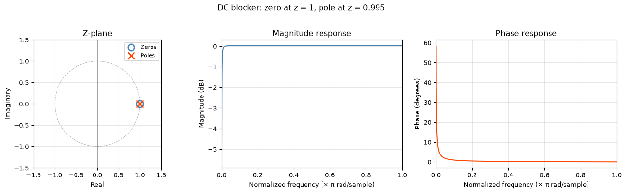
DC blocker
Classic high-pass configuration: set the zero at angle 0 degrees, radius 1.0 (a zero at \(z = 1\)), and the pole at angle 0 degrees, radius 0.995. This blocks DC while passing everything else. The closer the pole is to the zero, the narrower the transition band.
Allpass filter
Set a zero outside the unit circle (e.g., radius 1.11, angle 60 degrees) and a pole inside at the reciprocal radius (radius 0.9, angle 60 degrees). The magnitude response is approximately flat – only the phase changes. This is the allpass principle: for every zero at radius \(r\), place a pole at \(1/r\) at the same angle.
Connection to filter design
Classical filter design functions like scipy.signal.butter, cheby1, and ellip work by computing pole and zero locations that satisfy a given magnitude specification:
Butterworth places poles evenly on a circle in the s-plane, then maps them to the z-plane via the bilinear transform. For a lowpass design, all zeros end up at \(z = -1\) (Nyquist). The result is a maximally flat passband.
Chebyshev Type I allows ripple in the passband, which lets the poles move onto an ellipse – achieving a sharper transition for the same filter order.
Elliptic (Cauer) adds zeros in the stopband too, producing equiripple in both passband and stopband. This gives the sharpest transition of any classical design for a given order.
The explorer above shows the fundamental mechanism: every feature in the frequency response – every peak, notch, and slope – traces back to a specific pole or zero in the z-plane.
For reproducible work, here is the same computation in Python using scipy.signal.
Static pole-zero plot in Python
import numpy as npimport matplotlib.pyplot as pltfrom scipy.signal import freqz, tf2zpk# Define a simple filter: DC blocker# H(z) = (1 - z^{-1}) / (1 - 0.995 z^{-1})b = [1, -1] # numerator coefficients (zero at z=1)a = [1, -0.995] # denominator coefficients (pole at z=0.995)# Get poles and zerosz, p, k = tf2zpk(b, a)# Frequency responsew, h = freqz(b, a, worN=1024)fig, axes = plt.subplots(1, 3, figsize=(14, 4))# Z-planeax = axes[0]theta = np.linspace(0, 2* np.pi, 200)ax.plot(np.cos(theta), np.sin(theta), 'k--', alpha=0.3, linewidth=0.8)ax.plot(np.real(z), np.imag(z), 'o', markersize=10, markerfacecolor='none', markeredgecolor='steelblue', markeredgewidth=2, label='Zeros')ax.plot(np.real(p), np.imag(p), 'x', markersize=10, markeredgecolor='orangered', markeredgewidth=2, label='Poles')ax.axhline(0, color='grey', linewidth=0.5)ax.axvline(0, color='grey', linewidth=0.5)ax.set_xlim(-1.5, 1.5)ax.set_ylim(-1.5, 1.5)ax.set_aspect('equal')ax.set_xlabel('Real')ax.set_ylabel('Imaginary')ax.set_title('Z-plane')ax.legend(fontsize=8)ax.grid(True, alpha=0.3)# Magnitudeax = axes[1]ax.plot(w / np.pi, 20* np.log10(np.abs(h)), 'steelblue', linewidth=1.5)ax.set_xlabel('Normalized frequency (× π rad/sample)')ax.set_ylabel('Magnitude (dB)')ax.set_title('Magnitude response')ax.set_xlim(0, 1)ax.grid(True, alpha=0.3)# Phaseax = axes[2]ax.plot(w / np.pi, np.angle(h, deg=True), 'orangered', linewidth=1.5)ax.set_xlabel('Normalized frequency (× π rad/sample)')ax.set_ylabel('Phase (degrees)')ax.set_title('Phase response')ax.set_xlim(0, 1)ax.grid(True, alpha=0.3)fig.suptitle('DC blocker: zero at z = 1, pole at z = 0.995', fontsize=12, y=1.02)fig.tight_layout()plt.show()
/tmp/ipykernel_3380/1530387719.py:41: RuntimeWarning: divide by zero encountered in log10
  ax.plot(w / np.pi, 20 * np.log10(np.abs(h)), 'steelblue', linewidth=1.5)
To explore interactively in a Jupyter notebook, wrap the above in a function and use ipywidgets sliders – or simply adjust b and a and re-run the cell.
Source Code
---title: "Pole-Zero Explorer"subtitle: "Interactive exploration of how pole and zero placement shapes the frequency response"---The frequency response of a digital filter is completely determined by the locations of its poles and zeros in the z-plane. This interactive tool lets you explore that relationship by placing and moving poles and zeros, watching the magnitude and phase response change in real time.::: {.callout-note title="Prerequisites"}This page assumes familiarity with:- [The z-domain](../../basics/04-z-domain.qmd): transfer functions, poles, zeros, and the unit circle- [Filter design](../../basics/06-filter-design.qmd): how filter specifications map to pole-zero placement:::## Interactive explorerUse the sliders below to position poles and zeros in the z-plane. The transfer function is:$$H(z) = \frac{\prod_i (z - z_i)}{\prod_i (z - p_i)}$$where the frequency response is $H(e^{j\omega})$, evaluated on the unit circle. Since we want real-valued filter coefficients, poles and zeros appear in conjugate pairs.### Controls```{ojs}//| echo: false// --- Pole controls ---viewof poleRadius = Inputs.range([0, 1.3], { value: 0.95, step: 0.005, label: "Pole radius"})viewof poleAngle = Inputs.range([0, 180], { value: 45, step: 1, label: "Pole angle (degrees)"})// --- Zero controls ---viewof zeroRadius = Inputs.range([0, 2.0], { value: 1.0, step: 0.005, label: "Zero radius"})viewof zeroAngle = Inputs.range([0, 180], { value: 180, step: 1, label: "Zero angle (degrees)"})// --- Second pair toggle ---viewof showSecondPair = Inputs.toggle({ label: "Add second pole-zero pair", value: false})``````{ojs}//| echo: false// Second pair controls (only visible when toggled on)viewof poleRadius2 = Inputs.range([0, 1.3], { value: 0.9, step: 0.005, label: "Pole 2 radius", disabled: !showSecondPair})viewof poleAngle2 = Inputs.range([0, 180], { value: 90, step: 1, label: "Pole 2 angle (degrees)", disabled: !showSecondPair})viewof zeroRadius2 = Inputs.range([0, 2.0], { value: 1.0, step: 0.005, label: "Zero 2 radius", disabled: !showSecondPair})viewof zeroAngle2 = Inputs.range([0, 180], { value: 0, step: 1, label: "Zero 2 angle (degrees)", disabled: !showSecondPair})```### Preset configurations```{ojs}//| echo: false// Preset buttons using Inputs.buttonviewof preset = Inputs.radio( ["Custom", "DC blocker", "Resonator", "Notch filter", "Allpass"], { value: "Custom", label: "Preset" })``````{ojs}//| echo: false// Apply presets by updating the description textpresetDescription = { const descriptions = { "Custom": "Adjust the sliders freely.", "DC blocker": "Zero at z=1 (angle 0, radius 1), pole at z=0.995 (angle 0, radius 0.995). Blocks the DC component.", "Resonator": "Pole near the unit circle at 45 degrees (radius 0.99, angle 45). Creates a sharp resonance peak.", "Notch filter": "Zero on the unit circle at 60 degrees. Creates a deep null at that frequency.", "Allpass": "Zero outside the unit circle (radius 1.11), pole inside at the reciprocal radius (0.9), same angle. Magnitude is flat; only phase changes." }; return descriptions[preset];}```::: {.callout-tip title="Preset hint"}```{ojs}//| echo: falsemd`${presetDescription}**To apply a preset**, set the sliders to match. The presets suggest configurations. The sliders give you full control.````:::### Z-plane and frequency response```{ojs}//| echo: false// Convert angles from degrees to radianspoleAngleRad = poleAngle * Math.PI / 180zeroAngleRad = zeroAngle * Math.PI / 180poleAngleRad2 = poleAngle2 * Math.PI / 180zeroAngleRad2 = zeroAngle2 * Math.PI / 180// Build arrays of poles and zeros (conjugate pairs)poles = { const p = []; // First pair p.push({ re: poleRadius * Math.cos(poleAngleRad), im: poleRadius * Math.sin(poleAngleRad) }); if (poleAngle > 0 && poleAngle < 180) { p.push({ re: poleRadius * Math.cos(poleAngleRad), im: -poleRadius * Math.sin(poleAngleRad) }); } // Second pair (if enabled) if (showSecondPair) { p.push({ re: poleRadius2 * Math.cos(poleAngleRad2), im: poleRadius2 * Math.sin(poleAngleRad2) }); if (poleAngle2 > 0 && poleAngle2 < 180) { p.push({ re: poleRadius2 * Math.cos(poleAngleRad2), im: -poleRadius2 * Math.sin(poleAngleRad2) }); } } return p;}zeros = { const z = []; // First pair z.push({ re: zeroRadius * Math.cos(zeroAngleRad), im: zeroRadius * Math.sin(zeroAngleRad) }); if (zeroAngle > 0 && zeroAngle < 180) { z.push({ re: zeroRadius * Math.cos(zeroAngleRad), im: -zeroRadius * Math.sin(zeroAngleRad) }); } // Second pair (if enabled) if (showSecondPair) { z.push({ re: zeroRadius2 * Math.cos(zeroAngleRad2), im: zeroRadius2 * Math.sin(zeroAngleRad2) }); if (zeroAngle2 > 0 && zeroAngle2 < 180) { z.push({ re: zeroRadius2 * Math.cos(zeroAngleRad2), im: -zeroRadius2 * Math.sin(zeroAngleRad2) }); } } return z;}// Check stabilityisStable = poles.every(p => Math.sqrt(p.re * p.re + p.im * p.im) < 1.0)``````{ojs}//| echo: false// Stability indicatormd`**System is ${isStable ? "stable" : "UNSTABLE"}** ${isStable ? "" : "(pole outside unit circle — magnitude response diverges)"}```````{ojs}//| echo: false// Compute frequency response: H(e^{jw}) = prod(e^{jw} - z_i) / prod(e^{jw} - p_i)freqResponse = { const N = 512; const result = []; for (let k = 0; k <= N; k++) { const w = Math.PI * k / N; // 0 to pi const ejw_re = Math.cos(w); const ejw_im = Math.sin(w); // Numerator: product of (e^{jw} - z_i) let num_re = 1, num_im = 0; for (const z of zeros) { const diff_re = ejw_re - z.re; const diff_im = ejw_im - z.im; const new_re = num_re * diff_re - num_im * diff_im; const new_im = num_re * diff_im + num_im * diff_re; num_re = new_re; num_im = new_im; } // Denominator: product of (e^{jw} - p_i) let den_re = 1, den_im = 0; for (const p of poles) { const diff_re = ejw_re - p.re; const diff_im = ejw_im - p.im; const new_re = den_re * diff_re - den_im * diff_im; const new_im = den_re * diff_im + den_im * diff_re; den_re = new_re; den_im = new_im; } // H = num / den (complex division) const den_mag2 = den_re * den_re + den_im * den_im; const h_re = (num_re * den_re + num_im * den_im) / den_mag2; const h_im = (num_im * den_re - num_re * den_im) / den_mag2; const mag = Math.sqrt(h_re * h_re + h_im * h_im); const mag_dB = 20 * Math.log10(Math.max(mag, 1e-10)); const phase = Math.atan2(h_im, h_re) * 180 / Math.PI; result.push({ frequency: w / Math.PI, // normalized 0 to 1 magnitude_dB: mag_dB, phase_deg: phase }); } return result;}``````{ojs}//| echo: false// --- Z-plane plot ---{ // Unit circle points const circlePoints = []; for (let i = 0; i <= 100; i++) { const angle = 2 * Math.PI * i / 100; circlePoints.push({ x: Math.cos(angle), y: Math.sin(angle) }); } return Plot.plot({ title: "Z-plane", width: 450, height: 450, aspectRatio: 1, x: { domain: [-1.6, 1.6], label: "Real" }, y: { domain: [-1.6, 1.6], label: "Imaginary" }, marks: [ // Axes Plot.ruleX([0], { stroke: "#999", strokeWidth: 0.5 }), Plot.ruleY([0], { stroke: "#999", strokeWidth: 0.5 }), // Unit circle Plot.line(circlePoints, { x: "x", y: "y", stroke: "#999", strokeWidth: 1, strokeDasharray: "4,3" }), // Zeros (open circles) Plot.dot(zeros, { x: "re", y: "im", r: 8, stroke: "steelblue", strokeWidth: 2, fill: "none", symbol: "circle" }), // Poles (crosses) Plot.dot(poles, { x: "re", y: "im", r: 8, stroke: "orangered", strokeWidth: 2, fill: "none", symbol: "times" }), // Legend markers Plot.text([{ x: 1.1, y: 1.45 }], { x: "x", y: "y", text: d => "x Poles", fill: "orangered", fontSize: 12, textAnchor: "start" }), Plot.text([{ x: 1.1, y: 1.25 }], { x: "x", y: "y", text: d => "o Zeros", fill: "steelblue", fontSize: 12, textAnchor: "start" }) ] });}``````{ojs}//| echo: false// --- Magnitude response plot ---Plot.plot({ title: "Magnitude response", width: 640, height: 300, x: { label: "Normalized frequency (× π rad/sample)", domain: [0, 1] }, y: { label: "Magnitude (dB)", domain: [ Math.min(-40, Math.min(...freqResponse.map(d => d.magnitude_dB)) - 5), Math.max(20, Math.max(...freqResponse.map(d => d.magnitude_dB)) + 5) ]}, marks: [ Plot.ruleY([0], { stroke: "#999", strokeWidth: 0.5, strokeDasharray: "4,3" }), Plot.line(freqResponse, { x: "frequency", y: "magnitude_dB", stroke: "steelblue", strokeWidth: 2 }), Plot.gridY({ stroke: "#ddd", strokeWidth: 0.5 }), Plot.gridX({ stroke: "#ddd", strokeWidth: 0.5 }) ]})``````{ojs}//| echo: false// --- Phase response plot ---Plot.plot({ title: "Phase response", width: 640, height: 250, x: { label: "Normalized frequency (× π rad/sample)", domain: [0, 1] }, y: { label: "Phase (degrees)", domain: [-180, 180] }, marks: [ Plot.ruleY([0], { stroke: "#999", strokeWidth: 0.5, strokeDasharray: "4,3" }), Plot.line(freqResponse, { x: "frequency", y: "phase_deg", stroke: "orangered", strokeWidth: 2 }), Plot.gridY({ stroke: "#ddd", strokeWidth: 0.5 }), Plot.gridX({ stroke: "#ddd", strokeWidth: 0.5 }) ]})```## Guided explorationsTry these configurations and observe how the frequency response changes.::: {.callout-tip title="Resonance sharpness"}Set the pole angle to 45 degrees and sweep the radius from 0.5 to 0.99. Watch how the resonance peak narrows and grows as the pole approaches the unit circle. At radius 0.99, the peak is extremely sharp -- this is how a digital resonator works.:::::: {.callout-tip title="Notch depth"}Place a zero on the unit circle (radius = 1.0) at any angle. The magnitude drops to exactly zero at that frequency -- a perfect notch. Now move the zero slightly off the unit circle (radius = 0.95 or 1.05) and watch the notch become shallower. Only zeros exactly on the unit circle produce true nulls.:::::: {.callout-tip title="Instability"}Move the pole outside the unit circle (radius > 1.0). The system becomes unstable: the magnitude response diverges. In a real filter, this would cause the output to grow without bound. This is why filter design tools always constrain poles to lie strictly inside the unit circle.:::::: {.callout-tip title="DC blocker"}Classic high-pass configuration: set the zero at angle 0 degrees, radius 1.0 (a zero at $z = 1$), and the pole at angle 0 degrees, radius 0.995. This blocks DC while passing everything else. The closer the pole is to the zero, the narrower the transition band.:::::: {.callout-tip title="Allpass filter"}Set a zero outside the unit circle (e.g., radius 1.11, angle 60 degrees) and a pole inside at the reciprocal radius (radius 0.9, angle 60 degrees). The magnitude response is approximately flat -- only the phase changes. This is the allpass principle: for every zero at radius $r$, place a pole at $1/r$ at the same angle.:::## Connection to filter designClassical filter design functions like `scipy.signal.butter`, `cheby1`, and `ellip` work by computing pole and zero locations that satisfy a given magnitude specification:- **Butterworth** places poles evenly on a circle in the s-plane, then maps them to the z-plane via the bilinear transform. For a lowpass design, all zeros end up at $z = -1$ (Nyquist). The result is a maximally flat passband.- **Chebyshev Type I** allows ripple in the passband, which lets the poles move onto an ellipse -- achieving a sharper transition for the same filter order.- **Elliptic (Cauer)** adds zeros in the stopband too, producing equiripple in both passband and stopband. This gives the sharpest transition of any classical design for a given order.The explorer above shows the fundamental mechanism: every feature in the frequency response -- every peak, notch, and slope -- traces back to a specific pole or zero in the z-plane.For the full treatment, see [Filter design](../../basics/06-filter-design.qmd).## Python equivalentFor reproducible work, here is the same computation in Python using `scipy.signal`.```{python}#| code-fold: true#| code-summary: "Static pole-zero plot in Python"import numpy as npimport matplotlib.pyplot as pltfrom scipy.signal import freqz, tf2zpk# Define a simple filter: DC blocker# H(z) = (1 - z^{-1}) / (1 - 0.995 z^{-1})b = [1, -1] # numerator coefficients (zero at z=1)a = [1, -0.995] # denominator coefficients (pole at z=0.995)# Get poles and zerosz, p, k = tf2zpk(b, a)# Frequency responsew, h = freqz(b, a, worN=1024)fig, axes = plt.subplots(1, 3, figsize=(14, 4))# Z-planeax = axes[0]theta = np.linspace(0, 2* np.pi, 200)ax.plot(np.cos(theta), np.sin(theta), 'k--', alpha=0.3, linewidth=0.8)ax.plot(np.real(z), np.imag(z), 'o', markersize=10, markerfacecolor='none', markeredgecolor='steelblue', markeredgewidth=2, label='Zeros')ax.plot(np.real(p), np.imag(p), 'x', markersize=10, markeredgecolor='orangered', markeredgewidth=2, label='Poles')ax.axhline(0, color='grey', linewidth=0.5)ax.axvline(0, color='grey', linewidth=0.5)ax.set_xlim(-1.5, 1.5)ax.set_ylim(-1.5, 1.5)ax.set_aspect('equal')ax.set_xlabel('Real')ax.set_ylabel('Imaginary')ax.set_title('Z-plane')ax.legend(fontsize=8)ax.grid(True, alpha=0.3)# Magnitudeax = axes[1]ax.plot(w / np.pi, 20* np.log10(np.abs(h)), 'steelblue', linewidth=1.5)ax.set_xlabel('Normalized frequency (× π rad/sample)')ax.set_ylabel('Magnitude (dB)')ax.set_title('Magnitude response')ax.set_xlim(0, 1)ax.grid(True, alpha=0.3)# Phaseax = axes[2]ax.plot(w / np.pi, np.angle(h, deg=True), 'orangered', linewidth=1.5)ax.set_xlabel('Normalized frequency (× π rad/sample)')ax.set_ylabel('Phase (degrees)')ax.set_title('Phase response')ax.set_xlim(0, 1)ax.grid(True, alpha=0.3)fig.suptitle('DC blocker: zero at z = 1, pole at z = 0.995', fontsize=12, y=1.02)fig.tight_layout()plt.show()```To explore interactively in a Jupyter notebook, wrap the above in a function and use `ipywidgets` sliders -- or simply adjust `b` and `a` and re-run the cell.