Filter design by flocking, where gradients get stuck
Nature’s optimiser
A flock of starlings has no leader and no plan, yet it moves as one, wheeling around predators and settling on a roost. Each bird follows a few simple rules: match your neighbours, avoid collisions, and stay with the group (Reynolds 1987). Field measurements show each bird tracks a roughly fixed number of nearest neighbours rather than a fixed distance, which is what keeps the flock cohesive as it stretches and turns (Ballerini et al. 2008). Kennedy and Eberhart turned that idea into an optimiser: a swarm of candidate solutions, each pulled toward its own best memory and the swarm’s best find, searching a problem space the way a flock searches the sky (Kennedy and Eberhart 1995).
This page uses Particle Swarm Optimization (PSO) for a job that gradient methods do badly: designing IIR filters, whose error surfaces have many local minima. We contrast it with the gradient descent that underlies LMS adaptive filtering, show PSO escaping a trap that defeats the gradient, and use it to design a stable biquad. The embedded companion page asks the harder question: can the swarm itself run on a microcontroller?
Prerequisites
This topic assumes familiarity with IIR filters and stability and the z-domain. It is a natural companion to adaptive filtering, which solves the convex (FIR) case with gradients; here we take on the non-convex case.
Why gradients are not always enough
The LMS algorithm adjusts filter coefficients by walking downhill on the mean-squared-error surface. For an FIR filter that surface is a single quadratic bowl: there is one minimum, and walking downhill always finds it. LMS is the right tool, and a swarm would be overkill.
The picture changes for IIR filters. Because the coefficients appear in the denominator, the error surface as a function of the coefficients is non-convex: it has multiple local minima separated by ridges. A gradient method walks into whichever valley it started nearest and stops, even if a far deeper valley exists elsewhere. The same happens with any objective that is not differentiable, such as matching a magnitude mask with a hard stopband constraint.
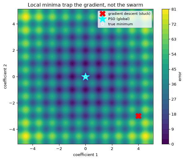
The Rastrigin function is the textbook caricature of such a surface: a single global minimum at the origin, buried in a regular lattice of local minima. It makes the failure of gradient descent visible.
Figure 1: The Rastrigin error surface (a stand-in for an IIR coefficient surface). Gradient descent from a poor start (red) stalls in the nearest local minimum; the PSO swarm (cyan) reaches the global minimum at the origin.
The PSO algorithm
A swarm is a set of particles, each a candidate solution \(x_i\) with a velocity \(v_i\). Every particle remembers the best position it has personally visited, \(p_i\) (its cognitive memory), and the whole swarm shares the best position anyone has found, \(g\) (the social knowledge). Each step, the velocity is nudged toward both, then the particle moves:
where \(r_1, r_2\) are fresh uniform random numbers in \([0, 1]\) drawn every step. The three weights set the character of the search:
\(\omega\) (inertia) keeps a particle moving in its current direction; high \(\omega\) explores, low \(\omega\) converges. The inertia term was not in the original swarm; Shi and Eberhart added it to balance exploration against convergence (Shi and Eberhart 1998).
\(c_1\) (cognitive) pulls a particle back toward its own best find.
\(c_2\) (social) pulls it toward the swarm’s best.
There is no gradient anywhere in this update. The swarm only ever evaluates the objective, which is why it works on surfaces that are non-convex, noisy, or not even differentiable. The implementation is in pso.py; the core loop is about a dozen lines.
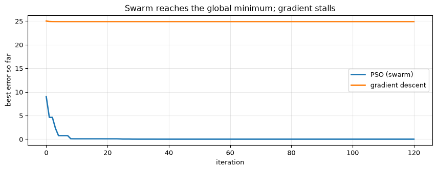
Figure 2: Convergence on the Rastrigin surface. The swarm drives the error to zero; gradient descent flattens out early at the value of its local minimum.
PSO for filter design
To design a filter with PSO, a particle is a coefficient vector and the fitness is how badly that filter misses the target. For a biquad the particle is \([b_0, b_1, b_2, a_1, a_2]\) and the fitness is the mean-squared error between its magnitude response and a desired one.
The one subtlety unique to IIR design is stability: a coefficient set with poles outside the unit circle is not just a bad filter, it is an unusable one. We keep the swarm honest with a stability wall, returning a large penalty for any unstable particle (the second-order Schur-Cohn conditions \(|a_2| < 1\) and \(|a_1| < 1 + a_2\)). The swarm learns to avoid that region.
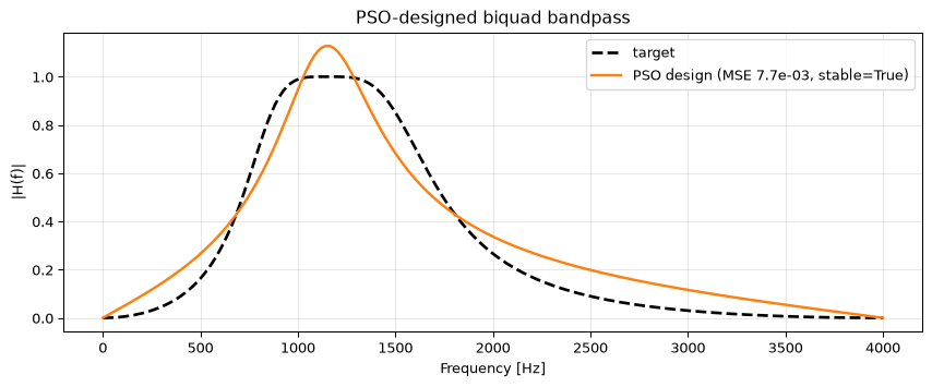
Figure 3: A biquad designed by PSO to match a target bandpass magnitude response. The swarm finds a stable coefficient set whose response tracks the target.
For this simple, closed-form-designable bandpass a conventional design (scipy.signal.butter) would of course be faster and exact. PSO earns its place when there is no closed-form designer: matching an arbitrary measured response, designing under a non-standard error norm, jointly optimising a multi-section filter with coupled constraints, or tuning a filter against a hardware-in-the-loop measurement where the only thing you can compute is the objective, not its gradient.
Cousins, briefly
PSO is one member of a family of nature-inspired, gradient-free optimisers, and the others show up in filter and signal work too:
Genetic algorithms (GA) evolve a population by selection, crossover, and mutation. They handle discrete and mixed search spaces well, for example choosing FIR tap quantisation levels or filter structures, where PSO’s continuous velocity update is a less natural fit.
Ant colony optimization (ACO) builds solutions from pheromone-weighted paths and suits combinatorial problems such as sensor or frequency assignment in spectrum sensing.
All three trade the guarantees of convex optimisation for the ability to search rugged, non-differentiable spaces. Which one wins is problem-specific and usually settled empirically.
Open questions and honest limits
PSO is powerful precisely because it assumes so little, and that same generality is the source of its limits.
No convergence guarantee. Unlike gradient descent on a convex function, PSO offers no proof it will find the global optimum, or any bound on how close it gets. It usually works well; it can also stagnate.
Hyperparameter sensitivity. The inertia and acceleration weights (\(\omega, c_1, c_2\)) strongly affect behaviour. Poor choices give premature convergence (the swarm collapses too early) or no convergence at all. Constriction-factor and adaptive-inertia variants reduce but do not remove this tuning burden.
Stochastic, so not repeatable without a seed. Two runs differ unless the random generator is fixed. Reporting a single lucky run is dishonest; the right practice is multiple seeded restarts and a distribution of outcomes.
Cost. Each iteration evaluates the objective once per particle. For an expensive fitness (a long simulation, or a filtering pass over real data) the population cost adds up, which is exactly the tension explored on the embedded page.
None of this disqualifies PSO. It marks where it is the right tool (rugged surfaces, no gradient, design-time budget) and where a gradient method or a closed-form designer is simply better.
References
Ballerini, M., N. Cabibbo, R. Candelier, A. Cavagna, E. Cisbani, I. Giardina, V. Lecomte, et al. 2008. “Interaction Ruling Animal Collective Behavior Depends on Topological Rather Than Metric Distance.”Proceedings of the National Academy of Sciences 105 (4): 1232–37.
Kennedy, James, and Russell Eberhart. 1995. “Particle Swarm Optimization.” In Proceedings of the IEEE International Conference on Neural Networks (ICNN), 4:1942–48. https://doi.org/10.1109/ICNN.1995.488968.
Reynolds, Craig W. 1987. “Flocks, Herds and Schools: A Distributed Behavioral Model.” In Proceedings of the 14th Annual Conference on Computer Graphics and Interactive Techniques (SIGGRAPH), 25–34.
Shi, Yuhui, and Russell Eberhart. 1998. “A Modified Particle Swarm Optimizer.” In Proceedings of the IEEE International Conference on Evolutionary Computation (ICEC), 69–73. https://doi.org/10.1109/ICEC.1998.699146.
Source Code
---title: "Particle Swarm Optimization for Filter Design"subtitle: "Filter design by flocking, where gradients get stuck"---::: {.callout-tip title="Nature's optimiser" appearance="simple"}A flock of starlings has no leader and no plan, yet it moves as one, wheeling around predators and settling on a roost. Each bird follows a few simple rules: match your neighbours, avoid collisions, and stay with the group [@reynolds1987flocks]. Field measurements show each bird tracks a roughly fixed number of nearest neighbours rather than a fixed distance, which is what keeps the flock cohesive as it stretches and turns [@ballerini2008interaction]. Kennedy and Eberhart turned that idea into an optimiser: a swarm of candidate solutions, each pulled toward its own best memory and the swarm's best find, searching a problem space the way a flock searches the sky [@kennedy1995particle].:::This page uses Particle Swarm Optimization (PSO) for a job that gradient methods do badly: designing **IIR filters**, whose error surfaces have many local minima. We contrast it with the gradient descent that underlies [LMS adaptive filtering](../adaptive-filtering/index.qmd), show PSO escaping a trap that defeats the gradient, and use it to design a stable biquad. The [embedded companion page](embedded.qmd) asks the harder question: can the swarm itself run on a microcontroller?::: {.callout-note title="Prerequisites"}This topic assumes familiarity with [IIR filters and stability](../../basics/06-filter-design.qmd) and the [z-domain](../../basics/04-z-domain.qmd). It is a natural companion to [adaptive filtering](../adaptive-filtering/index.qmd), which solves the convex (FIR) case with gradients; here we take on the non-convex case.:::---## Why gradients are not always enoughThe [LMS algorithm](../adaptive-filtering/index.qmd) adjusts filter coefficients by walking downhill on the mean-squared-error surface. For an **FIR** filter that surface is a single quadratic bowl: there is one minimum, and walking downhill always finds it. LMS is the right tool, and a swarm would be overkill.The picture changes for **IIR** filters. Because the coefficients appear in the denominator, the error surface as a function of the coefficients is **non-convex**: it has multiple local minima separated by ridges. A gradient method walks into whichever valley it started nearest and stops, even if a far deeper valley exists elsewhere. The same happens with any objective that is not differentiable, such as matching a magnitude mask with a hard stopband constraint.The Rastrigin function is the textbook caricature of such a surface: a single global minimum at the origin, buried in a regular lattice of local minima. It makes the failure of gradient descent visible.```{python}#| label: fig-surface#| fig-cap: "The Rastrigin error surface (a stand-in for an IIR coefficient surface). Gradient descent from a poor start (red) stalls in the nearest local minimum; the PSO swarm (cyan) reaches the global minimum at the origin."import numpy as npimport matplotlib.pyplot as pltfrom pso import pso, gradient_descentdef rastrigin(x): x = np.asarray(x)return10*len(x) + np.sum(x**2-10* np.cos(2* np.pi * x))bounds = [(-5.12, 5.12)] *2gbest, _, _ = pso(rastrigin, bounds, n_particles=40, n_iters=200, rng=np.random.default_rng(3))x_gd, _, _ = gradient_descent(rastrigin, [4.0, -3.0], bounds)g = np.linspace(-5.12, 5.12, 300)X, Y = np.meshgrid(g, g)Z =20+ X**2-10*np.cos(2*np.pi*X) + Y**2-10*np.cos(2*np.pi*Y)fig, ax = plt.subplots(figsize=(6.5, 5.5))cs = ax.contourf(X, Y, Z, levels=30, cmap="viridis")ax.plot(*x_gd, "X", color="red", ms=14, label="gradient descent (stuck)")ax.plot(*gbest, "*", color="cyan", ms=20, label="PSO (global)")ax.plot(0, 0, "o", color="white", ms=6, mfc="none", label="true minimum")ax.set_xlabel("coefficient 1"); ax.set_ylabel("coefficient 2")ax.set_title("Local minima trap the gradient, not the swarm")ax.legend(loc="upper right", fontsize=8)fig.colorbar(cs, ax=ax, label="error")fig.tight_layout(); plt.show()```---## The PSO algorithmA swarm is a set of **particles**, each a candidate solution $x_i$ with a velocity $v_i$. Every particle remembers the best position it has personally visited, $p_i$ (its *cognitive* memory), and the whole swarm shares the best position anyone has found, $g$ (the *social* knowledge). Each step, the velocity is nudged toward both, then the particle moves:$$v_i \leftarrow \underbrace{\omega\, v_i}_{\text{inertia}} + \underbrace{c_1 r_1 (p_i - x_i)}_{\text{cognitive}} + \underbrace{c_2 r_2 (g - x_i)}_{\text{social}}, \qquad x_i \leftarrow x_i + v_i,$$where $r_1, r_2$ are fresh uniform random numbers in $[0, 1]$ drawn every step. The three weights set the character of the search:- $\omega$ (**inertia**) keeps a particle moving in its current direction; high $\omega$ explores, low $\omega$ converges. The inertia term was not in the original swarm; Shi and Eberhart added it to balance exploration against convergence [@shi1998modified].- $c_1$ (**cognitive**) pulls a particle back toward its own best find.- $c_2$ (**social**) pulls it toward the swarm's best.There is no gradient anywhere in this update. The swarm only ever evaluates the objective, which is why it works on surfaces that are non-convex, noisy, or not even differentiable. The implementation is in [`pso.py`](pso.py); the core loop is about a dozen lines.```{python}#| label: fig-convergence#| fig-cap: "Convergence on the Rastrigin surface. The swarm drives the error to zero; gradient descent flattens out early at the value of its local minimum."_, _, hist_pso = pso(rastrigin, bounds, n_particles=40, n_iters=120, rng=np.random.default_rng(3))_, _, hist_gd = gradient_descent(rastrigin, [4.0, -3.0], bounds, n_iters=120)fig, ax = plt.subplots(figsize=(9, 3.6))ax.plot(hist_pso, label="PSO (swarm)", lw=2)ax.plot(hist_gd, label="gradient descent", lw=2)ax.set_xlabel("iteration"); ax.set_ylabel("best error so far")ax.set_title("Swarm reaches the global minimum; gradient stalls")ax.legend(); ax.grid(True, alpha=0.3)fig.tight_layout(); plt.show()```---## PSO for filter designTo design a filter with PSO, a particle **is** a coefficient vector and the fitness is how badly that filter misses the target. For a biquad the particle is $[b_0, b_1, b_2, a_1, a_2]$ and the fitness is the mean-squared error between its magnitude response and a desired one.The one subtlety unique to IIR design is **stability**: a coefficient set with poles outside the unit circle is not just a bad filter, it is an unusable one. We keep the swarm honest with a stability wall, returning a large penalty for any unstable particle (the second-order Schur-Cohn conditions $|a_2| < 1$ and $|a_1| < 1 + a_2$). The swarm learns to avoid that region.```{python}#| label: fig-iir#| fig-cap: "A biquad designed by PSO to match a target bandpass magnitude response. The swarm finds a stable coefficient set whose response tracks the target."from scipy import signalfrom pso import design_iir_pso, iir_is_stablefs =8000freqs = np.linspace(0, fs/2, 200)sos_target = signal.butter(2, [800, 1600], btype="band", fs=fs, output="sos")_, h_target = signal.sosfreqz(sos_target, worN=freqs, fs=fs)target_mag = np.abs(h_target)sos, err, _ = design_iir_pso(freqs, target_mag, fs, rng=np.random.default_rng(2))_, h_pso = signal.sosfreqz(sos, worN=freqs, fs=fs)stable = iir_is_stable(sos[0, 4], sos[0, 5])fig, ax = plt.subplots(figsize=(9, 3.8))ax.plot(freqs, target_mag, "k--", lw=2, label="target")ax.plot(freqs, np.abs(h_pso), color="C1", lw=1.8, label=f"PSO design (MSE {err:.1e}, stable={stable})")ax.set_xlabel("Frequency [Hz]"); ax.set_ylabel("|H(f)|")ax.set_title("PSO-designed biquad bandpass")ax.legend(); ax.grid(True, alpha=0.3)fig.tight_layout(); plt.show()```For this simple, closed-form-designable bandpass a conventional design (`scipy.signal.butter`) would of course be faster and exact. PSO earns its place when there is **no closed-form designer**: matching an arbitrary measured response, designing under a non-standard error norm, jointly optimising a multi-section filter with coupled constraints, or tuning a filter against a hardware-in-the-loop measurement where the only thing you can compute is the objective, not its gradient.---## Cousins, brieflyPSO is one member of a family of nature-inspired, gradient-free optimisers, and the others show up in filter and signal work too:- **Genetic algorithms (GA)** evolve a population by selection, crossover, and mutation. They handle discrete and mixed search spaces well, for example choosing FIR tap quantisation levels or filter structures, where PSO's continuous velocity update is a less natural fit.- **Ant colony optimization (ACO)** builds solutions from pheromone-weighted paths and suits combinatorial problems such as sensor or frequency assignment in spectrum sensing.All three trade the guarantees of convex optimisation for the ability to search rugged, non-differentiable spaces. Which one wins is problem-specific and usually settled empirically.---## Open questions and honest limitsPSO is powerful precisely because it assumes so little, and that same generality is the source of its limits.- **No convergence guarantee.** Unlike gradient descent on a convex function, PSO offers no proof it will find the global optimum, or any bound on how close it gets. It usually works well; it can also stagnate.- **Hyperparameter sensitivity.** The inertia and acceleration weights ($\omega, c_1, c_2$) strongly affect behaviour. Poor choices give premature convergence (the swarm collapses too early) or no convergence at all. Constriction-factor and adaptive-inertia variants reduce but do not remove this tuning burden.- **Stochastic, so not repeatable without a seed.** Two runs differ unless the random generator is fixed. Reporting a single lucky run is dishonest; the right practice is multiple seeded restarts and a distribution of outcomes.- **Cost.** Each iteration evaluates the objective once per particle. For an expensive fitness (a long simulation, or a filtering pass over real data) the population cost adds up, which is exactly the tension explored on the [embedded page](embedded.qmd).None of this disqualifies PSO. It marks where it is the right tool (rugged surfaces, no gradient, design-time budget) and where a gradient method or a closed-form designer is simply better.---## References::: {#refs}:::