A causal digital filter delays different frequency components by different amounts. This is not just a time shift. It distorts the waveform shape. Peaks spread, sharp edges soften asymmetrically, and the temporal relationships between signal components change. For many applications (biomedical signal analysis, vibration monitoring, feature extraction) this phase distortion is unacceptable.
Forward-backward filtering eliminates phase distortion entirely by filtering the signal twice: once forward in time, once backward. The result has the squared magnitude response of the original filter and exactly zero phase shift at all frequencies. The price: it requires the entire signal in advance. You cannot do this in real time.
Prerequisites
This topic assumes familiarity with filter design (IIR filters, group delay) and frequency-domain analysis. The group delay discussion provides the theoretical background on why linear-phase FIR filters are sometimes preferred over IIR filters.
Why phase matters
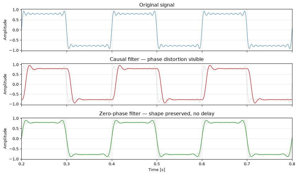
Consider a signal composed of two frequency components with a specific temporal relationship, say, a narrow pulse built from harmonics. A filter that shifts these harmonics by different amounts reassembles them into a different shape.
import numpy as npimport matplotlib.pyplot as pltfrom scipy import signal as sigfs =1000t = np.arange(2000) / fs# Pulse-like signal from harmonicsx = np.zeros_like(t)for k inrange(1, 20, 2): x += (1.0/ k) * np.sin(2* np.pi * k *5* t)# Lowpass IIR filtersos = sig.butter(4, 50, fs=fs, output='sos')# Causal filtering (forward only)y_causal = sig.sosfilt(sos, x)# Zero-phase filtering (forward-backward)y_zerophase = sig.sosfiltfilt(sos, x)fig, axes = plt.subplots(3, 1, figsize=(10, 6), sharex=True)axes[0].plot(t, x, 'C0', linewidth=0.8)axes[0].set_title('Original signal')axes[0].set_ylabel('Amplitude')axes[1].plot(t, x, 'C7', linewidth=0.5, alpha=0.5)axes[1].plot(t, y_causal, 'C3', linewidth=1.2)axes[1].set_title('Causal filter — phase distortion visible')axes[1].set_ylabel('Amplitude')axes[2].plot(t, x, 'C7', linewidth=0.5, alpha=0.5)axes[2].plot(t, y_zerophase, 'C2', linewidth=1.2)axes[2].set_title('Zero-phase filter — shape preserved, no delay')axes[2].set_ylabel('Amplitude')axes[2].set_xlabel('Time [s]')for ax in axes: ax.set_xlim(0.2, 0.8) ax.grid(True, alpha=0.3)fig.tight_layout()plt.show()
Figure 1: Causal filtering introduces phase distortion (time shift and waveform asymmetry). Zero-phase filtering preserves the original waveform shape.
The causal filter shifts and distorts the waveform. The zero-phase filter preserves the shape and timing of every feature.
How forward-backward filtering works
The algorithm is straightforward:
Forward pass: filter \(x[n]\) with \(H(z)\) to produce \(y_f[n]\)
Reverse: time-reverse \(y_f[n]\) to get \(y_f[-n]\)
Backward pass: filter \(y_f[-n]\) with \(H(z)\) again to produce \(y_b[n]\)
Reverse again: time-reverse \(y_b[n]\) to get the output \(y[n]\)
The phase of \(H(e^{j\omega})\) is exactly cancelled by the conjugate phase of the backward pass. What remains is the squared magnitude, always real and non-negative, hence zero phase.
Tip
The squared magnitude means the effective filter is “sharper” than you might expect. A 4th-order Butterworth filtered forward-backward has an 8th-order magnitude rolloff. Design for the single-pass order, knowing the effective order will be doubled.
SciPy implementation
SciPy provides two functions for zero-phase filtering:
scipy.signal.filtfilt(b, a, x): for transfer function form
scipy.signal.sosfiltfilt(sos, x): for second-order sections (preferred for numerical stability)
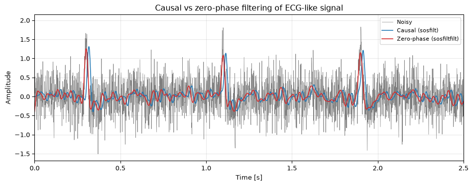
Figure 2: Comparison of causal vs zero-phase IIR lowpass on noisy ECG-like data. The zero-phase output has no delay and preserves peak timing, critical for biomedical applications.
Magnitude response comparison
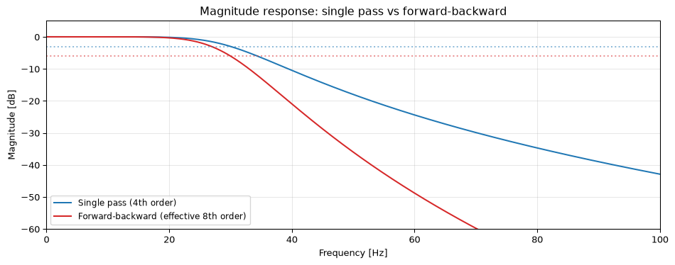
The forward-backward pass squares the magnitude response. This has practical consequences for filter specification:
Figure 3: Single-pass vs forward-backward magnitude response. The -3 dB point of the single-pass filter becomes the -6 dB point after forward-backward filtering. The effective rolloff is twice as steep.
If you want the -3 dB point of the forward-backward filter at a specific frequency \(f_c\), design the single-pass filter with a slightly higher cutoff. SciPy’s sosfiltfilt does not adjust for this automatically. You need to compensate yourself. For a Butterworth filter of order \(N\), the correction factor is:
This comes from requiring the forward–backward magnitude \(|H(\omega_c)|^2 = 1/\sqrt{2}\) (its \(-3\) dB point); for a Butterworth response \(|H(\omega)|^2 = 1/\!\left(1 + (\omega/\omega_\text{design})^{2N}\right)\) this gives \((\omega_c/\omega_\text{design})^{2N} = \sqrt{2} - 1\). The correction is modest but not negligible, about 12% at \(N = 4\), falling to ~6% at \(N = 8\), and is often tuned empirically.
FIR alternative: linear phase
Forward-backward filtering is not the only way to avoid phase distortion. A symmetric FIR filter has exactly linear phase, which corresponds to a pure time delay. The waveform shape is preserved, just shifted.
The trade-off:
Property
Forward-backward IIR
Linear-phase FIR
Phase distortion
Zero
Zero (constant delay)
Time delay
None
\((N-1)/2\) samples
Real-time capable
No
Yes
Filter order for sharp cutoff
Low (effective 2N)
High (hundreds of taps)
Edge effects
Yes (startup/end transients)
Yes (group delay at edges)
For offline analysis, forward-backward IIR is usually preferable: lower order, no delay, sharp cutoff. For real-time applications, a linear-phase FIR is the standard choice: you accept a fixed delay but get causal operation.
Edge effects and padding
Forward-backward filtering requires handling signal boundaries. When the forward pass reaches the end of the signal, the filter’s internal state contains transient energy that has nowhere to go. The backward pass then starts from this corrupted state, and the transient propagates back into the signal.
SciPy’s filtfilt and sosfiltfilt mitigate this by padding the signal before filtering and trimming afterwards. The padlen parameter controls how many samples of padding are added (default is 3 * max(len(a), len(b))). The padding method reflects the signal at the boundaries.
For short signals or aggressive filters (low cutoff, high order), the default padding may not be sufficient. Increasing padlen or manually padding the signal can help, but there is no perfect solution. Some edge corruption is inherent to the method.
Open questions
Minimum-phase alternative. Rather than achieving zero phase via forward-backward filtering, an alternative is to design a minimum-phase filter that concentrates its group delay at low frequencies and has the fastest possible impulse response. Minimum-phase filters are causal and have less delay than linear-phase FIR filters of comparable performance, but they still introduce some phase distortion. Whether this distortion is acceptable depends on the application.
Non-causal filtering in real-time. Forward-backward filtering is fundamentally non-causal, but some real-time systems approximate it using a look-ahead buffer: delay the output by \(D\) samples and use future input samples to approximate the backward pass. This gives “nearly zero” phase within the passband at the cost of a fixed latency. How much latency is needed for a given approximation quality is application-dependent and not well characterised in the literature for arbitrary filter designs.
Source Code
---title: "Zero-Phase Filtering"subtitle: "Filtering without phase distortion"---A causal digital filter delays different frequency components by different amounts. This is not just a time shift. It distorts the waveform shape. Peaks spread, sharp edges soften asymmetrically, and the temporal relationships between signal components change. For many applications (biomedical signal analysis, vibration monitoring, feature extraction) this phase distortion is unacceptable.**Forward-backward filtering** eliminates phase distortion entirely by filtering the signal twice: once forward in time, once backward. The result has the squared magnitude response of the original filter and exactly zero phase shift at all frequencies. The price: it requires the entire signal in advance. You cannot do this in real time.::: {.callout-note title="Prerequisites"}This topic assumes familiarity with [filter design](../../basics/06-filter-design.qmd) (IIR filters, group delay) and [frequency-domain analysis](../../basics/05-frequency-domain.qmd). The [group delay discussion](../../basics/06-filter-design.qmd) provides the theoretical background on why linear-phase FIR filters are sometimes preferred over IIR filters.:::---## Why phase mattersConsider a signal composed of two frequency components with a specific temporal relationship, say, a narrow pulse built from harmonics. A filter that shifts these harmonics by different amounts reassembles them into a different shape.```{python}#| label: fig-phase-distortion#| fig-cap: "Causal filtering introduces phase distortion (time shift and waveform asymmetry). Zero-phase filtering preserves the original waveform shape."import numpy as npimport matplotlib.pyplot as pltfrom scipy import signal as sigfs =1000t = np.arange(2000) / fs# Pulse-like signal from harmonicsx = np.zeros_like(t)for k inrange(1, 20, 2): x += (1.0/ k) * np.sin(2* np.pi * k *5* t)# Lowpass IIR filtersos = sig.butter(4, 50, fs=fs, output='sos')# Causal filtering (forward only)y_causal = sig.sosfilt(sos, x)# Zero-phase filtering (forward-backward)y_zerophase = sig.sosfiltfilt(sos, x)fig, axes = plt.subplots(3, 1, figsize=(10, 6), sharex=True)axes[0].plot(t, x, 'C0', linewidth=0.8)axes[0].set_title('Original signal')axes[0].set_ylabel('Amplitude')axes[1].plot(t, x, 'C7', linewidth=0.5, alpha=0.5)axes[1].plot(t, y_causal, 'C3', linewidth=1.2)axes[1].set_title('Causal filter — phase distortion visible')axes[1].set_ylabel('Amplitude')axes[2].plot(t, x, 'C7', linewidth=0.5, alpha=0.5)axes[2].plot(t, y_zerophase, 'C2', linewidth=1.2)axes[2].set_title('Zero-phase filter — shape preserved, no delay')axes[2].set_ylabel('Amplitude')axes[2].set_xlabel('Time [s]')for ax in axes: ax.set_xlim(0.2, 0.8) ax.grid(True, alpha=0.3)fig.tight_layout()plt.show()```The causal filter shifts and distorts the waveform. The zero-phase filter preserves the shape and timing of every feature.---## How forward-backward filtering worksThe algorithm is straightforward:1. **Forward pass:** filter $x[n]$ with $H(z)$ to produce $y_f[n]$2. **Reverse:** time-reverse $y_f[n]$ to get $y_f[-n]$3. **Backward pass:** filter $y_f[-n]$ with $H(z)$ again to produce $y_b[n]$4. **Reverse again:** time-reverse $y_b[n]$ to get the output $y[n]$The effective transfer function is:$$H_{\text{eff}}(e^{j\omega}) = H(e^{j\omega}) \cdot H(e^{-j\omega}) = |H(e^{j\omega})|^2$$The phase of $H(e^{j\omega})$ is exactly cancelled by the conjugate phase of the backward pass. What remains is the squared magnitude, always real and non-negative, hence zero phase.::: {.callout-tip}The squared magnitude means the effective filter is "sharper" than you might expect. A 4th-order Butterworth filtered forward-backward has an 8th-order magnitude rolloff. Design for the single-pass order, knowing the effective order will be doubled.:::---## SciPy implementationSciPy provides two functions for zero-phase filtering:- `scipy.signal.filtfilt(b, a, x)`: for transfer function form- `scipy.signal.sosfiltfilt(sos, x)`: for second-order sections (preferred for numerical stability)```{python}#| label: fig-filtfilt-comparison#| fig-cap: "Comparison of causal vs zero-phase IIR lowpass on noisy ECG-like data. The zero-phase output has no delay and preserves peak timing, critical for biomedical applications."# Simulate ECG-like signalrng = np.random.default_rng(123)t_ecg = np.arange(3000) / fsecg = np.zeros_like(t_ecg)for beat in np.arange(0.3, 2.7, 0.8): ecg +=1.5* np.exp(-((t_ecg - beat) /0.01)**2) # R peak ecg -=0.3* np.exp(-((t_ecg - beat -0.05) /0.03)**2) # T waveecg +=0.4* rng.standard_normal(len(t_ecg))# 30 Hz lowpasssos_lp = sig.butter(4, 30, fs=fs, output='sos')ecg_causal = sig.sosfilt(sos_lp, ecg)ecg_zp = sig.sosfiltfilt(sos_lp, ecg)fig, ax = plt.subplots(figsize=(10, 4))ax.plot(t_ecg, ecg, 'C7', linewidth=0.5, label='Noisy')ax.plot(t_ecg, ecg_causal, 'C0', linewidth=1.2, label='Causal (sosfilt)')ax.plot(t_ecg, ecg_zp, 'C3', linewidth=1.2, label='Zero-phase (sosfiltfilt)')ax.set_xlim(0, 2.5)ax.set_xlabel('Time [s]')ax.set_ylabel('Amplitude')ax.legend(fontsize=8)ax.grid(True, alpha=0.3)ax.set_title('Causal vs zero-phase filtering of ECG-like signal')fig.tight_layout()plt.show()```---## Magnitude response comparisonThe forward-backward pass squares the magnitude response. This has practical consequences for filter specification:```{python}#| label: fig-magnitude-squared#| fig-cap: "Single-pass vs forward-backward magnitude response. The -3 dB point of the single-pass filter becomes the -6 dB point after forward-backward filtering. The effective rolloff is twice as steep."w, H_single = sig.sosfreqz(sos_lp, worN=4096, fs=fs)H_fb = np.abs(H_single)**2# Forward-backward = squared magnitudefig, ax = plt.subplots(figsize=(10, 4))ax.plot(w, 20*np.log10(np.maximum(np.abs(H_single), 1e-10)),'C0', linewidth=1.5, label='Single pass (4th order)')ax.plot(w, 20*np.log10(np.maximum(H_fb, 1e-10)),'C3', linewidth=1.5, label='Forward-backward (effective 8th order)')ax.axhline(-3, color='C0', linestyle=':', alpha=0.5)ax.axhline(-6, color='C3', linestyle=':', alpha=0.5)ax.set_xlabel('Frequency [Hz]')ax.set_ylabel('Magnitude [dB]')ax.set_xlim(0, 100)ax.set_ylim(-60, 5)ax.legend(fontsize=9)ax.grid(True, alpha=0.3)ax.set_title('Magnitude response: single pass vs forward-backward')fig.tight_layout()plt.show()```If you want the -3 dB point of the forward-backward filter at a specific frequency $f_c$, design the single-pass filter with a slightly higher cutoff. SciPy's `sosfiltfilt` does not adjust for this automatically. You need to compensate yourself. For a Butterworth filter of order $N$, the correction factor is:$$f_{c,\text{design}} = f_c \cdot \left(\sqrt{2} - 1\right)^{-1/(2N)}$$This comes from requiring the forward–backward magnitude $|H(\omega_c)|^2 = 1/\sqrt{2}$ (its $-3$ dB point); for a Butterworth response $|H(\omega)|^2 = 1/\!\left(1 + (\omega/\omega_\text{design})^{2N}\right)$ this gives $(\omega_c/\omega_\text{design})^{2N} = \sqrt{2} - 1$. The correction is modest but not negligible, about 12% at $N = 4$, falling to ~6% at $N = 8$, and is often tuned empirically.---## FIR alternative: linear phaseForward-backward filtering is not the only way to avoid phase distortion. A **symmetric FIR filter** has exactly linear phase, which corresponds to a pure time delay. The waveform shape is preserved, just shifted.The trade-off:| Property | Forward-backward IIR | Linear-phase FIR ||----------|:-:|:-:|| Phase distortion | Zero | Zero (constant delay) || Time delay | None | $(N-1)/2$ samples || Real-time capable | No | Yes || Filter order for sharp cutoff | Low (effective 2N) | High (hundreds of taps) || Edge effects | Yes (startup/end transients) | Yes (group delay at edges) |For offline analysis, forward-backward IIR is usually preferable: lower order, no delay, sharp cutoff. For real-time applications, a linear-phase FIR is the standard choice: you accept a fixed delay but get causal operation.---## Edge effects and paddingForward-backward filtering requires handling signal boundaries. When the forward pass reaches the end of the signal, the filter's internal state contains transient energy that has nowhere to go. The backward pass then starts from this corrupted state, and the transient propagates back into the signal.SciPy's `filtfilt` and `sosfiltfilt` mitigate this by **padding** the signal before filtering and trimming afterwards. The `padlen` parameter controls how many samples of padding are added (default is `3 * max(len(a), len(b))`). The padding method reflects the signal at the boundaries.For short signals or aggressive filters (low cutoff, high order), the default padding may not be sufficient. Increasing `padlen` or manually padding the signal can help, but there is no perfect solution. Some edge corruption is inherent to the method.---## Open questions**Minimum-phase alternative.** Rather than achieving zero phase via forward-backward filtering, an alternative is to design a minimum-phase filter that concentrates its group delay at low frequencies and has the fastest possible impulse response. Minimum-phase filters are causal and have less delay than linear-phase FIR filters of comparable performance, but they still introduce some phase distortion. Whether this distortion is acceptable depends on the application.**Non-causal filtering in real-time.** Forward-backward filtering is fundamentally non-causal, but some real-time systems approximate it using a look-ahead buffer: delay the output by $D$ samples and use future input samples to approximate the backward pass. This gives "nearly zero" phase within the passband at the cost of a fixed latency. How much latency is needed for a given approximation quality is application-dependent and not well characterised in the literature for arbitrary filter designs.