The chapters before this one built up the signal processing: sampling, filters, transforms, multirate, correlation. All of it was Python, running on a laptop with effectively unlimited time and memory. This closing chapter is about the other half of the workshop’s title, the metal: what changes when the same algorithms have to run on a small processor, in real time, on a power budget.
The good news is that the math does not change. A biquad is a biquad whether it runs in NumPy or on a Cortex-M4. What changes is the cost model. On a laptop you rarely count multiplies; on a microcontroller every cycle, every byte of RAM, and every microsecond of latency is visible. This chapter is the bridge: it explains the hardware landscape the workshop’s embedded companion pages target, so those pages can get on with the code.
Three places DSP runs
Historically there were two answers to “what chip do I run my DSP on,” and they pulled in opposite directions.
A general-purpose microcontroller is built for control: reading sensors, driving peripherals, handling interrupts, sipping power. It is excellent at talking to the world and mediocre at arithmetic, because it lacks the registers and instructions that make tight numerical loops fast.
A dedicated digital signal processor (the Analog Devices SHARC is the classic teaching example) is the mirror image. It is built to do multiply-accumulate all day: it can fetch two operands and compute in a single cycle, loop with no per-iteration overhead, address circular buffers in hardware, and carry extra guard bits in a wide accumulator so sums do not overflow. Some even bolt on fixed-function blocks for FIR, IIR, and FFT. The price is power draw, cost, and a programming model tuned for throughput rather than everyday tasks (Yiu 2014, ch. 21).
For years a product that needed both, say a connected audio device, carried both chips. The Cortex-M4 collapsed that split: it is a microcontroller with DSP extensions, a single-cycle MAC, SIMD (single instruction, multiple data: one operation applied to several packed values at once) on 8- and 16-bit data, saturating arithmetic, and (on the M4F) a single-precision floating-point unit, while keeping the low interrupt overhead and low power of an MCU. It is not as fast as a high-end dedicated DSP, but for the sample rates and filter orders in this workshop it is comfortably enough, and it is deterministic and cheap. That middle ground is where most of the workshop’s embedded pages live (the NUCLEO-F446RE is a Cortex-M4F).
General MCU
Cortex-M4(F)
Dedicated DSP (SHARC)
Single-cycle MAC
no
yes
yes
Circular / bit-reversed addressing
no
no (do it in software)
yes, in hardware
Double-width accumulator
no
partial (64-bit SMLAL, no guard bits)
yes (guard bits)
Floating-point
sometimes
yes (M4F, single precision)
yes
Interrupt overhead
low
low
high
Power
low
low
higher
Best at
control, peripherals
the middle ground
maximum throughput
Note
This workshop targets the middle ground (ESP32-S3 and NUCLEO-F446RE by default, with a broader capability ladder when a page is specifically about what cheaper or smaller parts can manage). The point is not that the Cortex-M4 is always the right answer, but that it is a good default for “real DSP on a small, cheap, low-power part.”
The MAC is the universal kernel
Look back through the workshop and almost every algorithm reduces to the same inner operation: multiply two numbers and add the result to a running sum. An FIR filter is a dot product of the signal with its coefficients. A biquad is five multiply-accumulates per sample. Correlation and matched filtering are dot products at every lag. The DFT is a sum of products. The multiply-accumulate (MAC) is the heartbeat of DSP, which is exactly why the hardware above is organised around making it fast.
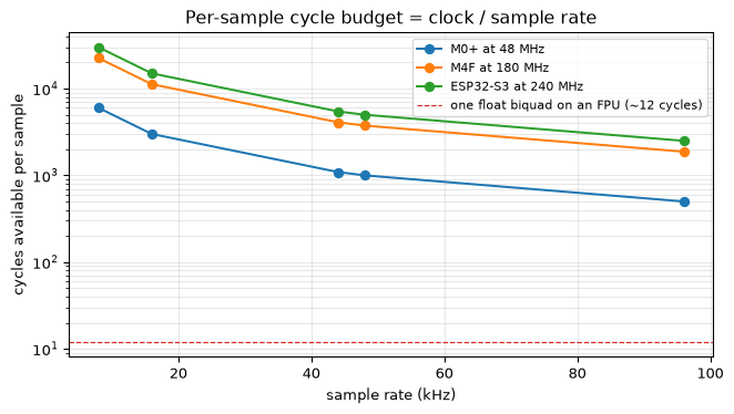
How fast matters in a specific, unforgiving way. Real-time DSP runs on a clock: a new sample arrives every \(1/f_s\) seconds, and the processing for it must finish before the next one lands. The figure of merit is therefore the per-sample cycle budget:
\[
\text{cycles per sample} = \frac{f_\text{clock}}{f_s}
\]
Show the code
import numpy as npimport matplotlib.pyplot as pltrates = np.array([8000, 16000, 44100, 48000, 96000])clocks = {"M0+ at 48 MHz": 48e6, "M4F at 180 MHz": 180e6, "ESP32-S3 at 240 MHz": 240e6}# Self-check: the budget at 180 MHz / 48 kHz is the 3750 cycles quoted on the biquad pageassertabs(180e6/48000-3750) <1e-6fig, ax = plt.subplots(figsize=(7, 4))for name, fclk in clocks.items(): ax.plot(rates /1000, fclk / rates, "o-", label=name)ax.axhline(12, color="C3", ls="--", lw=0.9, label="one float biquad on an FPU (~12 cycles)")ax.set_xlabel("sample rate (kHz)")ax.set_ylabel("cycles available per sample")ax.set_yscale("log")ax.set_title("Per-sample cycle budget = clock / sample rate")ax.legend(fontsize=8)ax.grid(True, which="both", alpha=0.3)fig.tight_layout()plt.show()
Figure 1: The per-sample cycle budget (processor clock divided by sample rate) for three targets across common audio sample rates. Even the tightest pairing here (a 48 MHz part at 96 kHz) leaves hundreds of cycles per sample, and the faster parts leave thousands; a biquad costs about a dozen, so the headroom is large until the sample rate climbs or the algorithm grows.
The subtle part is the word budget. What matters is not the average processing load but the worst case: if one sample in a thousand takes longer than \(1/f_s\), that is a dropped sample, an audible click, a corrupted measurement. This is why determinism is prized in DSP hardware. A dedicated DSP completes a MAC in one cycle, every time. A Cortex-M4 is nearly as predictable. A general MCU, where the same multiply can take 3 to 7 cycles depending on the operands, makes the worst case hard to pin down. At a CD sample rate of 44.1 kHz the budget is 22.67 microseconds per sample; you want to know, not hope, that your code fits.
For a worked example of how the cycle count for one filter is actually built up (and why a biquad costs about a dozen cycles rather than the nine its arithmetic suggests), see Counting the cycles on the biquad page.
Addressing: the tricks a DSP has and an MCU fakes
Two memory-addressing tricks separate a dedicated DSP from a Cortex-M4, and both show up constantly in DSP code.
Circular addressing. An FIR filter keeps the last \(N\) samples in a delay line. The naive way to advance it, shifting every sample down by one each time a new one arrives, costs \(N\) memory moves per sample. A dedicated DSP instead wraps a pointer around a fixed buffer in hardware, so the data never moves. The Cortex-M4 has no such mode, so embedded C does it in software with a modulo index, the circular buffer shown in the FIR example. The idea is the same; only the bookkeeping moves from hardware into your loop.
Bit-reversed addressing. The fast Fourier transform leaves its outputs in bit-reversed order, and a dedicated DSP can read them back in natural order for free with a special addressing mode. Again the Cortex-M4 does it in software, which is why CMSIS-DSP’s FFT functions include an explicit reordering step.
Numbers: float or fixed point
On a part with a floating-point unit (the M4F, the ESP32-S3) the easy and usual choice is single-precision float: the dynamic range is enormous, overflow is a non-issue in practice, and the code reads like the Python. Reach for fixed-point only when you have to: on a part with no FPU (a Cortex-M0+, an AVR), or when power or throughput demands the integer SIMD path.
Fixed-point trades that comfort for control. Values are stored as scaled integers (Q15, Q31), every multiply needs thought about where the binary point lands, sums need a wide enough accumulator not to overflow, and on overflow you must choose between wrapping (which tears a waveform apart) and saturating (which clips it gently). Those mechanics are general to all fixed-point DSP, not just one filter, so they live in the finite word-length effects topic, with the biquad as a worked instance.
Getting samples in and out
None of the arithmetic matters until real samples flow through it. The standard real-time structure is a timer-paced chain: a hardware timer triggers the ADC at exactly \(f_s\), DMA (direct memory access, hardware that moves samples between the converter and memory without the CPU) carries each conversion into memory, the processing runs in the transfer-complete interrupt, and the result goes out to a DAC. Pacing the input with a timer rather than a software loop is what keeps the sampling jitter-free, and the output has to be paced just as carefully. The biquad real-time I/O section works the whole chain end to end on a NUCLEO-F446RE, and the multirate page shows the same scaffolding driving a sample-rate converter.
Libraries do the hard part
You rarely hand-optimise this code. ARM’s CMSIS-DSP library ships tuned MAC loops, FIR and biquad filters, FFTs, and statistics for the Cortex-M, in float and in Q15/Q31, applying every scheduling and unrolling trick by hand so you do not have to. Espressif’s ESP-DSP does the same for the Xtensa cores in the ESP32 family. The skill worth having is not writing the assembly; it is understanding the cost model well enough to choose the right algorithm, the right number format, and the right sample rate, and then to read the library’s results critically.
Going further
This chapter is the conceptual map, and it is also the end of the Basics path. Where you go next depends on which direction pulls harder.
More metal. The territory behind this map is in the per-topic embedded companions, each taking one algorithm all the way to working C on real hardware: the biquad (the fullest treatment, including the cycle budget and the real-time chain), multirate, Goertzel tone detection, matched filtering, and the bio-inspired topics that stretch across the capability ladder, gammatone and Gabor filters.
For the hardware itself, Joseph Yiu’s Definitive Guide to ARM Cortex-M3 and Cortex-M4 Processors(Yiu 2014) is the standard reference for the DSP extensions and how to write efficient code against them. For the signal-processing software forms, Julius Smith’s Introduction to Digital Filters(Smith 2007) is the canonical free treatment.
Yiu, Joseph. 2014. The Definitive Guide to ARM Cortex-M3 and Cortex-M4 Processors. 3rd ed. Oxford: Newnes.
Source Code
---title: "DSP on a microcontroller"subtitle: "Where the math meets the metal"description-meta: "What changes when DSP algorithms leave the laptop: the cost model of a small processor, and the hardware landscape for real-time filtering on an MCU."---The chapters before this one built up the signal processing: sampling, filters, transforms, multirate, correlation. All of it was Python, running on a laptop with effectively unlimited time and memory. This closing chapter is about the other half of the workshop's title, the **metal**: what changes when the same algorithms have to run on a small processor, in real time, on a power budget.The good news is that the math does not change. A biquad is a biquad whether it runs in NumPy or on a Cortex-M4. What changes is the cost model. On a laptop you rarely count multiplies; on a microcontroller every cycle, every byte of RAM, and every microsecond of latency is visible. This chapter is the bridge: it explains the hardware landscape the workshop's embedded companion pages target, so those pages can get on with the code.## Three places DSP runsHistorically there were two answers to "what chip do I run my DSP on," and they pulled in opposite directions.A **general-purpose microcontroller** is built for control: reading sensors, driving peripherals, handling interrupts, sipping power. It is excellent at talking to the world and mediocre at arithmetic, because it lacks the registers and instructions that make tight numerical loops fast.A **dedicated digital signal processor** (the Analog Devices SHARC is the classic teaching example) is the mirror image. It is built to do multiply-accumulate all day: it can fetch two operands and compute in a single cycle, loop with no per-iteration overhead, address circular buffers in hardware, and carry extra guard bits in a wide accumulator so sums do not overflow. Some even bolt on fixed-function blocks for FIR, IIR, and FFT. The price is power draw, cost, and a programming model tuned for throughput rather than everyday tasks [@yiu2014, ch. 21].For years a product that needed both, say a connected audio device, carried both chips. The **Cortex-M4** collapsed that split: it is a microcontroller with **DSP extensions**, a single-cycle MAC, SIMD (single instruction, multiple data: one operation applied to several packed values at once) on 8- and 16-bit data, saturating arithmetic, and (on the M4F) a single-precision floating-point unit, while keeping the low interrupt overhead and low power of an MCU. It is not as fast as a high-end dedicated DSP, but for the sample rates and filter orders in this workshop it is comfortably enough, and it is deterministic and cheap. That middle ground is where most of the workshop's embedded pages live (the NUCLEO-F446RE is a Cortex-M4F).| | General MCU | Cortex-M4(F) | Dedicated DSP (SHARC) ||---|---|---|---|| Single-cycle MAC | no | yes | yes || Circular / bit-reversed addressing | no | no (do it in software) | yes, in hardware || Double-width accumulator | no | partial (64-bit `SMLAL`, no guard bits) | yes (guard bits) || Floating-point | sometimes | yes (M4F, single precision) | yes || Interrupt overhead | low | low | high || Power | low | low | higher || Best at | control, peripherals | the middle ground | maximum throughput |::: {.callout-note}This workshop targets the middle ground (ESP32-S3 and NUCLEO-F446RE by default, with a broader capability ladder when a page is specifically about what cheaper or smaller parts can manage). The point is not that the Cortex-M4 is always the right answer, but that it is a good default for "real DSP on a small, cheap, low-power part.":::## The MAC is the universal kernelLook back through the workshop and almost every algorithm reduces to the same inner operation: multiply two numbers and add the result to a running sum. An FIR filter is a dot product of the signal with its coefficients. A [biquad](09-biquad/index.qmd) is five multiply-accumulates per sample. [Correlation and matched filtering](11-convolution-correlation-modulation.qmd) are dot products at every lag. The DFT is a sum of products. The **multiply-accumulate (MAC)** is the heartbeat of DSP, which is exactly why the hardware above is organised around making it fast.How fast matters in a specific, unforgiving way. Real-time DSP runs on a clock: a new sample arrives every $1/f_s$ seconds, and the processing for it must finish before the next one lands. The figure of merit is therefore the **per-sample cycle budget**:$$\text{cycles per sample} = \frac{f_\text{clock}}{f_s}$$```{python}#| label: fig-cycle-budget#| fig-cap: "The per-sample cycle budget (processor clock divided by sample rate) for three targets across common audio sample rates. Even the tightest pairing here (a 48 MHz part at 96 kHz) leaves hundreds of cycles per sample, and the faster parts leave thousands; a biquad costs about a dozen, so the headroom is large until the sample rate climbs or the algorithm grows."import numpy as npimport matplotlib.pyplot as pltrates = np.array([8000, 16000, 44100, 48000, 96000])clocks = {"M0+ at 48 MHz": 48e6, "M4F at 180 MHz": 180e6, "ESP32-S3 at 240 MHz": 240e6}# Self-check: the budget at 180 MHz / 48 kHz is the 3750 cycles quoted on the biquad pageassertabs(180e6/48000-3750) <1e-6fig, ax = plt.subplots(figsize=(7, 4))for name, fclk in clocks.items(): ax.plot(rates /1000, fclk / rates, "o-", label=name)ax.axhline(12, color="C3", ls="--", lw=0.9, label="one float biquad on an FPU (~12 cycles)")ax.set_xlabel("sample rate (kHz)")ax.set_ylabel("cycles available per sample")ax.set_yscale("log")ax.set_title("Per-sample cycle budget = clock / sample rate")ax.legend(fontsize=8)ax.grid(True, which="both", alpha=0.3)fig.tight_layout()plt.show()```The subtle part is the word *budget*. What matters is not the *average* processing load but the *worst case*: if one sample in a thousand takes longer than $1/f_s$, that is a dropped sample, an audible click, a corrupted measurement. This is why **determinism** is prized in DSP hardware. A dedicated DSP completes a MAC in one cycle, every time. A Cortex-M4 is nearly as predictable. A general MCU, where the same multiply can take 3 to 7 cycles depending on the operands, makes the worst case hard to pin down. At a CD sample rate of 44.1 kHz the budget is 22.67 microseconds per sample; you want to know, not hope, that your code fits.For a worked example of how the cycle count for one filter is actually built up (and why a biquad costs about a dozen cycles rather than the nine its arithmetic suggests), see [Counting the cycles](09-biquad/embedded.qmd#counting-the-cycles) on the biquad page.## Addressing: the tricks a DSP has and an MCU fakesTwo memory-addressing tricks separate a dedicated DSP from a Cortex-M4, and both show up constantly in DSP code.**Circular addressing.** An FIR filter keeps the last $N$ samples in a delay line. The naive way to advance it, shifting every sample down by one each time a new one arrives, costs $N$ memory moves per sample. A dedicated DSP instead wraps a pointer around a fixed buffer in hardware, so the data never moves. The Cortex-M4 has no such mode, so embedded C does it in software with a modulo index, the **circular buffer** shown in the [FIR example](09-biquad/embedded.qmd#fir-comparison). The idea is the same; only the bookkeeping moves from hardware into your loop.**Bit-reversed addressing.** The fast Fourier transform leaves its outputs in bit-reversed order, and a dedicated DSP can read them back in natural order for free with a special addressing mode. Again the Cortex-M4 does it in software, which is why CMSIS-DSP's FFT functions include an explicit reordering step.## Numbers: float or fixed pointOn a part with a floating-point unit (the M4F, the ESP32-S3) the easy and usual choice is single-precision `float`: the dynamic range is enormous, overflow is a non-issue in practice, and the code reads like the Python. Reach for **fixed-point** only when you have to: on a part with no FPU (a Cortex-M0+, an AVR), or when power or throughput demands the integer SIMD path.Fixed-point trades that comfort for control. Values are stored as scaled integers (Q15, Q31), every multiply needs thought about where the binary point lands, sums need a wide enough accumulator not to overflow, and on overflow you must choose between wrapping (which tears a waveform apart) and saturating (which clips it gently). Those mechanics are general to all fixed-point DSP, not just one filter, so they live in the [finite word-length effects](../topics/finite-wordlength/index.qmd) topic, with the biquad as a worked instance.## Getting samples in and outNone of the arithmetic matters until real samples flow through it. The standard real-time structure is a **timer-paced chain**: a hardware timer triggers the ADC at exactly $f_s$, DMA (direct memory access, hardware that moves samples between the converter and memory without the CPU) carries each conversion into memory, the processing runs in the transfer-complete interrupt, and the result goes out to a DAC. Pacing the input with a timer rather than a software loop is what keeps the sampling jitter-free, and the output has to be paced just as carefully. The [biquad real-time I/O section](09-biquad/embedded.qmd#real-time-io-clocking-samples-in-and-out) works the whole chain end to end on a NUCLEO-F446RE, and the [multirate page](10-multirate/embedded.qmd) shows the same scaffolding driving a sample-rate converter.## Libraries do the hard partYou rarely hand-optimise this code. ARM's **CMSIS-DSP** library ships tuned MAC loops, FIR and biquad filters, FFTs, and statistics for the Cortex-M, in float and in Q15/Q31, applying every scheduling and unrolling trick by hand so you do not have to. Espressif's **ESP-DSP** does the same for the Xtensa cores in the ESP32 family. The skill worth having is not writing the assembly; it is understanding the cost model well enough to choose the right algorithm, the right number format, and the right sample rate, and then to read the library's results critically.## Going furtherThis chapter is the conceptual map, and it is also the end of the Basics path. Where you go next depends on which direction pulls harder.**More metal.** The territory behind this map is in the per-topic embedded companions, each taking one algorithm all the way to working C on real hardware: the [biquad](09-biquad/embedded.qmd) (the fullest treatment, including the cycle budget and the real-time chain), [multirate](10-multirate/embedded.qmd), [Goertzel tone detection](../topics/goertzel/embedded.qmd), [matched filtering](../topics/matched-filtering/embedded.qmd), and the bio-inspired topics that stretch across the capability ladder, [gammatone](../topics/gammatone-filters/embedded.qmd) and [Gabor](../topics/gabor-filters/embedded.qmd) filters.**More theory.** The guided arcs in [Topics](../topics/index.qmd) continue where Basics stops: [feature extraction](../topics/feature-extraction.qmd) picks up from Chapter 5's frequency domain, [noise & stochastic processing](../topics/noise-and-stochastic-processing.qmd) builds on Chapters 3 and 5, and [estimation & detection](../topics/estimation-and-detection.qmd) reads best after the noise arc. The two branches meet again at that last arc's capstone, a [voice pitch estimator](../topics/voice-pitch-estimator/index.qmd) that runs as a complete instrument on an ESP32.For the hardware itself, Joseph Yiu's *Definitive Guide to ARM Cortex-M3 and Cortex-M4 Processors* [@yiu2014] is the standard reference for the DSP extensions and how to write efficient code against them. For the signal-processing software forms, Julius Smith's *Introduction to Digital Filters* [@smith2007filters] is the canonical free treatment.## References::: {#refs}:::