Convolution, Correlation, and Modulation

Three ways signals combine

Three operations keep showing up whenever two signals interact: convolution, correlation, and modulation. They look different at first, but they are close cousins, and one idea ties them together: an operation that is a sliding-and-summing in one domain becomes a simple multiplication in the other. Convolution in time is multiplication in frequency; multiplication in time (modulation) is convolution in frequency. Correlation sits right next to convolution, differing only by a time flip.

You have already met convolution in Chapter 2 as the way an LTI filter acts on a signal. Here we recap it briefly, then build out its two relatives and the frequency-domain duality that unifies them.

Prerequisites

This chapter assumes discrete-time systems (convolution as LTI filtering, impulse response) and the frequency domain (the Fourier view, spectra). The correlation section connects forward to matched filtering, where these ideas are pushed into a detection algorithm.

Convolution, recapped

Convolution is the operation that combines an input with a system’s impulse response to produce the output. For two discrete sequences it is the sliding weighted sum

\[(x * h)[n] = \sum_{m=-\infty}^{\infty} x[m]\,h[n-m] = \sum_{m=-\infty}^{\infty} x[n-m]\,h[m].\]

The two forms are equal because convolution is commutative: $x * h = h * x$. The mechanics are flip-and-slide: reverse one sequence, slide it past the other, and at each shift sum the overlapping products.

There is a second way to see it that is worth keeping in your pocket: convolving two sequences is multiplying two polynomials. If $x$ and $h$ are the coefficient lists of two polynomials in $z^{-1}$, then $x * h$ is the coefficient list of their product. That is exactly why a longer filter “spreads” a signal: multiplying polynomials of degree $M$ and $N$ gives one of degree $M + N$.

import numpy as np
import matplotlib.pyplot as plt

x = np.array([0, 2, 1, 3])
h = np.array([1, 2, -3])      # h[n] = delta[n] + 2 delta[n-1] - 3 delta[n-2]
y = np.convolve(x, h)

# Verify against the hand-worked answer from the exercise set
expected = np.array([0, 2, 5, -1, 3, -9])
assert np.array_equal(y, expected), y
print("x * h =", y, " (length", len(y), "=", len(x), "+", len(h), "- 1 )")

fig, axes = plt.subplots(1, 3, figsize=(11, 3))
for ax, sig, title in [(axes[0], x, 'x[n]'), (axes[1], h, 'h[n]'), (axes[2], y, 'y[n] = (x * h)[n]')]:
    ax.stem(np.arange(len(sig)), sig, basefmt='k-')
    ax.set_title(title)
    ax.set_xlabel('n')
    ax.grid(True, alpha=0.3)
    ax.axhline(0, color='k', linewidth=0.5)
fig.tight_layout()
plt.show()

x * h = [ 0  2  5 -1  3 -9]  (length 6 = 4 + 3 - 1 )

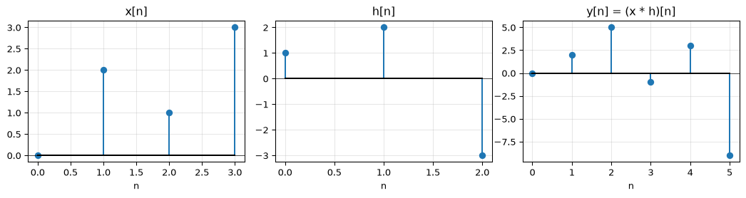
Figure 1: Flip-and-slide convolution of x = [0, 2, 1, 3] with h = [1, 2, -3]. Each output sample is the sum of the overlapping products at that shift; the result has length len(x) + len(h) - 1.

The algebra is worth doing once by hand. Flip $h$ to $[-3, 2, 1]$, slide it across $x$, and at each position sum the products: $y[2] = x[0]h[2] + x[1]h[1] + x[2]h[0] = 0 + 4 + 1 = 5$, and so on, giving $y = [0, 2, 5, -1, 3, -9]$.

A few properties earn their keep:

Property	Statement
Commutative	$x * h = h * x$
Associative	$x * (h * g) = (x * h) * g$
Distributive	$x * (h + g) = x * h + x * g$

The associativity is what lets you cascade filters in any order and lump them into one (the idea behind the cascade structures in the previous chapter).

The convolution theorem

The single most useful fact about convolution is its frequency-domain face. Convolution in time is multiplication in frequency:

\[x * h \;\longleftrightarrow\; X(\omega)\,H(\omega).\]

This is why filtering is so often described by a frequency response: passing a signal through a filter just multiplies its spectrum by $H(\omega)$. No new frequencies are created; the existing ones are only rescaled and phase-shifted. Hold on to this duality, because modulation is its mirror image.

Correlation

Correlation measures how similar two signals are as a function of how far you slide one past the other. Where convolution flips one signal before sliding, correlation does not. That single difference changes what the operation is for: convolution describes how a system reshapes a signal, while correlation asks “where does this pattern appear, and how strongly?”

Cross-correlation

For two real sequences, the cross-correlation at lag $\ell$ is the sliding dot product

\[(x \star h)[\ell] = \sum_{n=-\infty}^{\infty} x[n]\,h[n+\ell].\]

(For complex signals you conjugate the first: $x^*[n]\,h[n+\ell]$.) When the two signals line up, peaks meet peaks and troughs meet troughs; every product is positive and the sum is large. The lag where the cross-correlation peaks is the shift that best aligns them, which makes correlation the natural tool for finding a time delay:

\[\ell_\text{delay} = \arg\max_\ell\,(x \star h)[\ell].\]

rng = np.random.default_rng(0)

pulse = np.sin(2 * np.pi * np.linspace(0, 1, 20)) * np.hanning(20)
true_delay = 60
record = np.zeros(200)
record[true_delay:true_delay + len(pulse)] += pulse
record += 0.3 * rng.standard_normal(len(record))

# Slide the template across the record (full cross-correlation), then read the peak lag
xc = np.correlate(record, pulse, mode='valid')
est_delay = int(np.argmax(xc))
assert est_delay == true_delay, (est_delay, true_delay)
print("estimated delay =", est_delay, "samples (true:", true_delay, ")")

fig, axes = plt.subplots(2, 1, figsize=(10, 4.5))
axes[0].plot(record, 'C0', linewidth=0.7)
axes[0].axvspan(true_delay, true_delay + len(pulse), color='C1', alpha=0.2, label='pulse location')
axes[0].set_title('Noisy record with a hidden pulse')
axes[0].legend(fontsize=8); axes[0].set_ylabel('amplitude')
axes[1].plot(xc, 'C3', linewidth=1)
axes[1].axvline(est_delay, color='k', linestyle='--', linewidth=0.8)
axes[1].set_title(f'Cross-correlation peaks at lag {est_delay}')
axes[1].set_xlabel('lag'); axes[1].set_ylabel('similarity')
for ax in axes: ax.grid(True, alpha=0.3)
fig.tight_layout()
plt.show()

estimated delay = 60 samples (true: 60 )

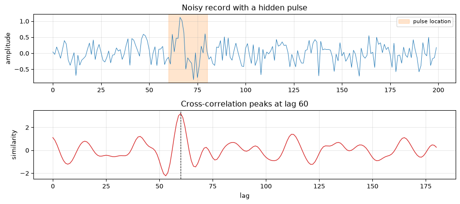
Figure 2: Cross-correlation finds an unknown delay. A short pulse is buried in noise 60 samples into a longer record; the cross-correlation of the record with a clean copy of the pulse peaks exactly at lag 60.

This is exactly the principle behind matched filtering: correlating a noisy record against a known template is the optimal way to detect that template in white noise. It is also how a microphone array estimates direction (correlate the two channels, read off the inter-microphone delay), which the beamforming topic builds on.

Autocorrelation

Autocorrelation is the cross-correlation of a signal with itself:

\[R_x[\ell] = \sum_{n=-\infty}^{\infty} x[n]\,x[n+\ell].\]

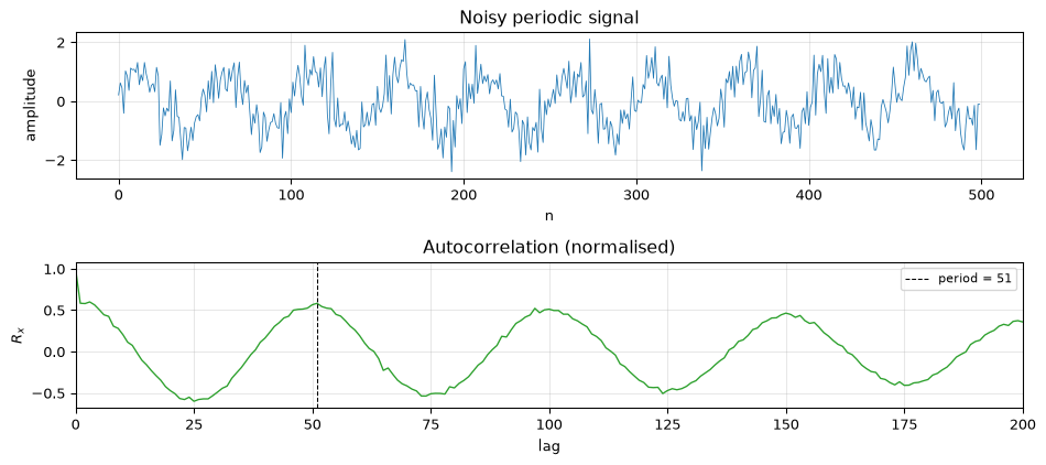
It answers “how self-similar is this signal at a lag of $\ell$?”, which is the question you ask to find hidden periodicity. A periodic signal repeats, so its autocorrelation peaks again at every multiple of the period, even when noise hides the period in the raw waveform. Two properties fall out immediately:

It is symmetric: $R_x[\ell] = R_x[-\ell]$.
Its largest value is at zero lag: $|R_x[\ell]| \le R_x[0]$, because nothing matches a signal better than itself perfectly aligned.

rng = np.random.default_rng(1)
period = 50
n = np.arange(500)
sig = np.sin(2 * np.pi * n / period) + 0.6 * rng.standard_normal(len(n))

# Unbiased-ish autocorrelation via full correlation, normalised to R[0] = 1
ac = np.correlate(sig, sig, mode='full')
ac = ac[ac.size // 2:]          # keep non-negative lags
ac = ac / ac[0]

# Largest peak after lag 0 should land on the true period
search = ac[30:120]      # look past the central lobe for the first period peak
est_period = int(np.argmax(search)) + 30
assert ac[0] == 1.0 and abs(est_period - period) <= 1, (est_period, ac[0])
print("R_x[0] =", ac[0], " estimated period =", est_period, "(true:", period, ")")

fig, axes = plt.subplots(2, 1, figsize=(10, 4.5))
axes[0].plot(n, sig, 'C0', linewidth=0.6)
axes[0].set_title('Noisy periodic signal'); axes[0].set_ylabel('amplitude'); axes[0].set_xlabel('n')
lags = np.arange(len(ac))
axes[1].plot(lags, ac, 'C2', linewidth=1)
axes[1].axvline(est_period, color='k', linestyle='--', linewidth=0.8, label=f'period = {est_period}')
axes[1].set_title('Autocorrelation (normalised)'); axes[1].set_xlabel('lag'); axes[1].set_ylabel('$R_x$')
axes[1].set_xlim(0, 200); axes[1].legend(fontsize=8)
for ax in axes: ax.grid(True, alpha=0.3)
fig.tight_layout()
plt.show()

R_x[0] = 1.0  estimated period = 51 (true: 50 )

Figure 3: Autocorrelation exposes a period that is hard to see in noise. The waveform (top) is a 50-sample-period sine buried in noise; its autocorrelation (bottom) is symmetric, peaks at lag 0, and shows clear secondary peaks at every multiple of the period.

This is the autocorrelation route to pitch detection: the fundamental period shows up as the first strong autocorrelation peak away from zero, even when the fundamental is weaker than its harmonics.

Correlation is convolution with a flip

Correlation is not a separate machine; it is convolution with one signal reversed (and conjugated, for complex data):

\[x \star h = x^*(-n) * h.\]

For a symmetric kernel ($h[-n] = h[n]$) the flip does nothing, so convolution and correlation give the same result. That is the case worth remembering: when people say “convolving with a Gaussian,” correlation and convolution coincide because the Gaussian is symmetric. The frequency-domain version mirrors the convolution theorem,

\[x \star h \;\longleftrightarrow\; X^*(\omega)\,H(\omega),\]

so a cross-correlation is just as cheap to compute through the FFT as a convolution.

Modulation

Modulation is the mirror image of convolution. Where convolution multiplies spectra, multiplying two signals in time convolves their spectra:

\[x[n]\,c[n] \;\longleftrightarrow\; \tfrac{1}{2\pi}\,X(\omega) * C(\omega).\]

(The constant depends on your Fourier convention; the structure is what matters.) The most familiar case is amplitude modulation (AM), where a slow message rides on the amplitude of a fast carrier so it can be sent over the air.

Take a carrier $c(t) = A\sin(2\pi f_c t)$ and a message $m(t) = M\cos(2\pi f_m t + \phi)$ with $f_m \ll f_c$. Standard AM transmits the carrier multiplied by $(1 + m(t))$:

\[y(t) = \bigl[1 + M\cos(2\pi f_m t + \phi)\bigr]\,A\sin(2\pi f_c t).\]

We insist that $M < 1$ so that $1 + m(t)$ never goes negative. If $M > 1$ the envelope crosses zero and folds over: this is overmodulation, and a simple envelope detector can no longer recover the message. The value $M$ (for a single-tone message) is the modulation index, or depth of modulation.

Expand the product with the identity $2\sin a\cos b = \sin(a+b) + \sin(a-b)$ and the modulated signal splits into three pure tones:

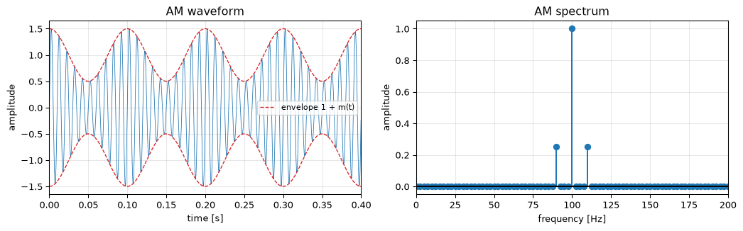
\[y(t) = A\sin(2\pi f_c t) + \frac{AM}{2}\Bigl[\sin\bigl(2\pi (f_c + f_m)t + \phi\bigr) + \sin\bigl(2\pi (f_c - f_m)t - \phi\bigr)\Bigr].\]

So the spectrum is the unchanged carrier at $f_c$ plus two sidebands at $f_c \pm f_m$, each of amplitude $AM/2$. That is the convolution-in-frequency picture made concrete: multiplying the message by the carrier took the message spectrum and copied it up to sit around $\pm f_c$.

fs = 4000
t = np.arange(0, 0.4, 1 / fs)
A, M, fc, fm = 1.0, 0.5, 100, 10

carrier = A * np.sin(2 * np.pi * fc * t)
message = M * np.cos(2 * np.pi * fm * t)
y = (1 + message) * carrier

# Spectrum
Y = np.abs(np.fft.rfft(y)) * 2 / len(y)
f = np.fft.rfftfreq(len(y), 1 / fs)

# Verify the three predicted lines: carrier at fc (amp ~A), sidebands at fc +/- fm (amp ~A*M/2)
def amp_at(freq):
    return Y[np.argmin(np.abs(f - freq))]
assert abs(amp_at(fc) - A) < 0.05, amp_at(fc)
for sf in (fc - fm, fc + fm):
    assert abs(amp_at(sf) - A * M / 2) < 0.05, (sf, amp_at(sf))
print(f"carrier {amp_at(fc):.2f} (~{A}), sidebands {amp_at(fc-fm):.2f}/{amp_at(fc+fm):.2f} (~{A*M/2})")

fig, axes = plt.subplots(1, 2, figsize=(11, 3.5))
axes[0].plot(t, y, 'C0', linewidth=0.6)
axes[0].plot(t, 1 + message, 'C3--', linewidth=1, label='envelope 1 + m(t)')
axes[0].plot(t, -(1 + message), 'C3--', linewidth=1)
axes[0].set_title('AM waveform'); axes[0].set_xlabel('time [s]'); axes[0].set_ylabel('amplitude')
axes[0].legend(fontsize=8); axes[0].set_xlim(0, 0.4)
axes[1].stem(f, Y, basefmt='k-')
axes[1].set_title('AM spectrum'); axes[1].set_xlabel('frequency [Hz]'); axes[1].set_ylabel('amplitude')
axes[1].set_xlim(0, 200)
for ax in axes: ax.grid(True, alpha=0.3)
fig.tight_layout()
plt.show()

carrier 1.00 (~1.0), sidebands 0.25/0.25 (~0.25)

Figure 4: Amplitude modulation. Left: a 100 Hz carrier whose envelope traces the 10 Hz message (modulation index 0.5). Right: the spectrum is the carrier at 100 Hz plus two sidebands at 90 and 110 Hz, each of amplitude A*M/2.

A real message is not one tone but a band of them. By Fourier decomposition each component spawns its own pair of sidebands, so the whole message spectrum appears twice in the modulated signal: shifted up to sit just above $f_c$ (the upper sideband) and reflected just below it (the lower sideband), with the carrier standing tall in the middle. The carrier carries no information itself, yet it holds more power than both sidebands combined, which is why power-efficient schemes (suppressed-carrier, single-sideband) drop or halve it.

Exercises

Exercise 1: Convolution by hand

A system has impulse response $h[n] = \delta[n] + 2\delta[n-1] - 3\delta[n-2]$. Compute its response to the input $x = [0, 2, 1, 3]$ (samples at $n = 0,1,2,3$) by convolution.

Solution. Flip $h$ to $[-3, 2, 1]$, slide it across $x$, and sum the overlapping products at each shift:

\[ \begin{aligned} y[0] &= x[0]h[0] = 0\\ y[1] &= x[0]h[1] + x[1]h[0] = 0 + 2 = 2\\ y[2] &= x[0]h[2] + x[1]h[1] + x[2]h[0] = 0 + 4 + 1 = 5\\ y[3] &= x[1]h[2] + x[2]h[1] + x[3]h[0] = -6 + 2 + 3 = -1\\ y[4] &= x[2]h[2] + x[3]h[1] = -3 + 6 = 3\\ y[5] &= x[3]h[2] = -9 \end{aligned} \]

So $y = [0, 2, 5, -1, 3, -9]$, length $4 + 3 - 1 = 6$. (This is the worked example computed in the first code cell above.)

Exercise 2: Amplitude modulation

A carrier $10\cos(2\pi\,10^6 t)\ \text{V}$ is amplitude modulated by a second wave $0.3\cos(2\pi\,10^3 t)\ \text{V}$. Find (a) the depth of modulation, (b) the upper and lower side frequencies, (c) the amplitude of the side frequencies, and (d) the combined sideband power as a fraction of the carrier power.

Solution. Carrier amplitude $A = 10$, carrier frequency $f_c = 10^6\ \text{Hz}$, modulation index $M = 0.3$, message frequency $f_m = 10^3\ \text{Hz}$.

Depth of modulation $= M = 0.3 = \mathbf{30\%}$ (the modulating amplitude relative to the $1$ in $1 + m(t)$).
Side frequencies $f_c \pm f_m = 10^6 \pm 10^3 = \mathbf{1.001\ \text{MHz}}$ and $\mathbf{0.999\ \text{MHz}}$.
Side-frequency amplitude $= \dfrac{AM}{2} = \dfrac{10 \cdot 0.3}{2} = \mathbf{1.5\ \text{V}}$.
With carrier power $P_c = A^2/R = 10^2/R$ and each sideband $P_s = (AM/2)^2/R = 1.5^2/R$, the combined sideband power relative to the carrier is

\[\frac{2P_s}{P_c} = 2\cdot\frac{1.5^2}{10^2} = 0.045 = \mathbf{4.5\%}.\]

Almost all the transmitted power sits in the (information-free) carrier, the headline weakness of standard AM.

Exercise 3: Sketch the convolutions

Sketch $y[n] = x[n] * h[n]$ for:

$x = [1, 1]$ and $h = [1, \tfrac{1}{2}]$ (both starting at $n=0$).
$x = [1, 1]$ and $h = [1, 1, 1, 1]$.
$x = \delta[n] - \delta[n-2]$ and $h = [1, 1, 1, 1]$.

Solutions.

$y = [1, \tfrac{3}{2}, \tfrac{1}{2}]$.
$y = [1, 2, 2, 2, 1]$ (a trapezoid: the running sum of a 2-wide box over a 4-wide box).
$y = h[n] - h[n-2] = [1, 1, 0, 0, -1, -1]$ (the box, minus a copy shifted by 2).

You can confirm any of these with np.convolve, for example np.convolve([1, 1], [1, 1, 1, 1]).

Going further

The three operations are one family seen from different sides, and each opens into a topic of its own.

Correlation as a detector. Sliding a known template past a noisy record and reading the peak is the cheapest good detector there is. Pushed to its optimal form it becomes the matched filter; applied to a signal against itself it becomes the autocorrelation pitch tracker in pitch detection.
Modulation as frequency shifting. Multiplying by a carrier moves a spectrum bodily up the frequency axis. The same trick run in reverse (multiply by a carrier, then lowpass) shifts a band back down to baseband, the heart of every radio receiver and of the lock-in amplifier. The short-time Fourier transform leans on the dual idea of windowing as multiplication in time.
The duality itself. Convolution in one domain is multiplication in the other, full stop. Once that is reflex, half of DSP is reading a problem in whichever domain makes the operation a multiply.

References

The operations and their properties follow standard treatments in Oppenheim and Schafer (Oppenheim and Schafer 2010) and Proakis and Manolakis (Proakis and Manolakis 2007); the AM analysis is the classic single-tone derivation found in any communications text.

Oppenheim, Alan V., and Ronald W. Schafer. 2010. Discrete-Time Signal Processing. 3rd ed. Pearson.

Proakis, John G., and Dimitris G. Manolakis. 2007. Digital Signal Processing: Principles, Algorithms, and Applications. 4th ed. Pearson.

--- title: "Convolution, Correlation, and Modulation" subtitle: "Three ways signals combine" --- Three operations keep showing up whenever two signals interact: **convolution**, **correlation**, and **modulation**. They look different at first, but they are close cousins, and one idea ties them together: an operation that is a sliding-and-summing in one domain becomes a simple multiplication in the other. Convolution in time is multiplication in frequency; multiplication in time (modulation) is convolution in frequency. Correlation sits right next to convolution, differing only by a time flip. You have already met convolution in [Chapter 2](02-discrete-time.qmd) as the way an LTI filter acts on a signal. Here we recap it briefly, then build out its two relatives and the frequency-domain duality that unifies them. ::: {.callout-note title="Prerequisites"} This chapter assumes [discrete-time systems](02-discrete-time.qmd) (convolution as LTI filtering, impulse response) and the [frequency domain](05-frequency-domain.qmd) (the Fourier view, spectra). The correlation section connects forward to [matched filtering](../topics/matched-filtering/index.qmd), where these ideas are pushed into a detection algorithm. ::: <hr> ## Convolution, recapped Convolution is the operation that combines an input with a system's impulse response to produce the output. For two discrete sequences it is the sliding weighted sum $$(x * h)[n] = \sum_{m=-\infty}^{\infty} x[m]\,h[n-m] = \sum_{m=-\infty}^{\infty} x[n-m]\,h[m].$$ The two forms are equal because convolution is **commutative**: $x * h = h * x$. The mechanics are flip-and-slide: reverse one sequence, slide it past the other, and at each shift sum the overlapping products. There is a second way to see it that is worth keeping in your pocket: **convolving two sequences is multiplying two polynomials**. If $x$ and $h$ are the coefficient lists of two polynomials in $z^{-1}$, then $x * h$ is the coefficient list of their product. That is exactly why a longer filter "spreads" a signal: multiplying polynomials of degree $M$ and $N$ gives one of degree $M + N$. ```{python} #| label: fig-conv-mechanics #| fig-cap: "Flip-and-slide convolution of x = [0, 2, 1, 3] with h = [1, 2, -3]. Each output sample is the sum of the overlapping products at that shift; the result has length len(x) + len(h) - 1." import numpy as np import matplotlib.pyplot as plt x = np.array([0, 2, 1, 3]) h = np.array([1, 2, -3]) # h[n] = delta[n] + 2 delta[n-1] - 3 delta[n-2] y = np.convolve(x, h) # Verify against the hand-worked answer from the exercise set expected = np.array([0, 2, 5, -1, 3, -9]) assert np.array_equal(y, expected), y print("x * h =", y, " (length", len(y), "=", len(x), "+", len(h), "- 1 )") fig, axes = plt.subplots(1, 3, figsize=(11, 3)) for ax, sig, title in [(axes[0], x, 'x[n]'), (axes[1], h, 'h[n]'), (axes[2], y, 'y[n] = (x * h)[n]')]: ax.stem(np.arange(len(sig)), sig, basefmt='k-') ax.set_title(title) ax.set_xlabel('n') ax.grid(True, alpha=0.3) ax.axhline(0, color='k', linewidth=0.5) fig.tight_layout() plt.show() ``` The algebra is worth doing once by hand. Flip $h$ to $[-3, 2, 1]$, slide it across $x$, and at each position sum the products: $y[2] = x[0]h[2] + x[1]h[1] + x[2]h[0] = 0 + 4 + 1 = 5$, and so on, giving $y = [0, 2, 5, -1, 3, -9]$. A few properties earn their keep: | Property | Statement | |---|---| | Commutative | $x * h = h * x$ | | Associative | $x * (h * g) = (x * h) * g$ | | Distributive | $x * (h + g) = x * h + x * g$ | The associativity is what lets you cascade filters in any order and lump them into one (the idea behind the [cascade structures](07-filter-structures.qmd) in the previous chapter). ::: {.callout-important title="The convolution theorem"} The single most useful fact about convolution is its frequency-domain face. Convolution in time is **multiplication** in frequency: $$x * h \;\longleftrightarrow\; X(\omega)\,H(\omega).$$ This is why filtering is so often described by a frequency response: passing a signal through a filter just multiplies its spectrum by $H(\omega)$. No new frequencies are created; the existing ones are only rescaled and phase-shifted. Hold on to this duality, because modulation is its mirror image. ::: <hr> ## Correlation **Correlation** measures how similar two signals are as a function of how far you slide one past the other. Where convolution flips one signal before sliding, correlation does not. That single difference changes what the operation is *for*: convolution describes how a system reshapes a signal, while correlation asks "where does this pattern appear, and how strongly?" ### Cross-correlation For two real sequences, the cross-correlation at lag $\ell$ is the sliding dot product $$(x \star h)[\ell] = \sum_{n=-\infty}^{\infty} x[n]\,h[n+\ell].$$ (For complex signals you conjugate the first: $x^*[n]\,h[n+\ell]$.) When the two signals line up, peaks meet peaks and troughs meet troughs; every product is positive and the sum is large. The lag where the cross-correlation peaks is the shift that best aligns them, which makes correlation the natural tool for finding a **time delay**: $$\ell_\text{delay} = \arg\max_\ell\,(x \star h)[\ell].$$ ```{python} #| label: fig-xcorr-delay #| fig-cap: "Cross-correlation finds an unknown delay. A short pulse is buried in noise 60 samples into a longer record; the cross-correlation of the record with a clean copy of the pulse peaks exactly at lag 60." rng = np.random.default_rng(0) pulse = np.sin(2 * np.pi * np.linspace(0, 1, 20)) * np.hanning(20) true_delay = 60 record = np.zeros(200) record[true_delay:true_delay + len(pulse)] += pulse record += 0.3 * rng.standard_normal(len(record)) # Slide the template across the record (full cross-correlation), then read the peak lag xc = np.correlate(record, pulse, mode='valid') est_delay = int(np.argmax(xc)) assert est_delay == true_delay, (est_delay, true_delay) print("estimated delay =", est_delay, "samples (true:", true_delay, ")") fig, axes = plt.subplots(2, 1, figsize=(10, 4.5)) axes[0].plot(record, 'C0', linewidth=0.7) axes[0].axvspan(true_delay, true_delay + len(pulse), color='C1', alpha=0.2, label='pulse location') axes[0].set_title('Noisy record with a hidden pulse') axes[0].legend(fontsize=8); axes[0].set_ylabel('amplitude') axes[1].plot(xc, 'C3', linewidth=1) axes[1].axvline(est_delay, color='k', linestyle='--', linewidth=0.8) axes[1].set_title(f'Cross-correlation peaks at lag {est_delay}') axes[1].set_xlabel('lag'); axes[1].set_ylabel('similarity') for ax in axes: ax.grid(True, alpha=0.3) fig.tight_layout() plt.show() ``` This is exactly the principle behind [matched filtering](../topics/matched-filtering/index.qmd): correlating a noisy record against a known template is the optimal way to detect that template in white noise. It is also how a microphone array estimates direction (correlate the two channels, read off the inter-microphone delay), which the [beamforming](../topics/beamforming/index.qmd) topic builds on. ### Autocorrelation **Autocorrelation** is the cross-correlation of a signal with itself: $$R_x[\ell] = \sum_{n=-\infty}^{\infty} x[n]\,x[n+\ell].$$ It answers "how self-similar is this signal at a lag of $\ell$?", which is the question you ask to find hidden periodicity. A periodic signal repeats, so its autocorrelation peaks again at every multiple of the period, even when noise hides the period in the raw waveform. Two properties fall out immediately: - It is **symmetric**: $R_x[\ell] = R_x[-\ell]$. - Its **largest value is at zero lag**: $|R_x[\ell]| \le R_x[0]$, because nothing matches a signal better than itself perfectly aligned. ```{python} #| label: fig-autocorr #| fig-cap: "Autocorrelation exposes a period that is hard to see in noise. The waveform (top) is a 50-sample-period sine buried in noise; its autocorrelation (bottom) is symmetric, peaks at lag 0, and shows clear secondary peaks at every multiple of the period." rng = np.random.default_rng(1) period = 50 n = np.arange(500) sig = np.sin(2 * np.pi * n / period) + 0.6 * rng.standard_normal(len(n)) # Unbiased-ish autocorrelation via full correlation, normalised to R[0] = 1 ac = np.correlate(sig, sig, mode='full') ac = ac[ac.size // 2:] # keep non-negative lags ac = ac / ac[0] # Largest peak after lag 0 should land on the true period search = ac[30:120] # look past the central lobe for the first period peak est_period = int(np.argmax(search)) + 30 assert ac[0] == 1.0 and abs(est_period - period) <= 1, (est_period, ac[0]) print("R_x[0] =", ac[0], " estimated period =", est_period, "(true:", period, ")") fig, axes = plt.subplots(2, 1, figsize=(10, 4.5)) axes[0].plot(n, sig, 'C0', linewidth=0.6) axes[0].set_title('Noisy periodic signal'); axes[0].set_ylabel('amplitude'); axes[0].set_xlabel('n') lags = np.arange(len(ac)) axes[1].plot(lags, ac, 'C2', linewidth=1) axes[1].axvline(est_period, color='k', linestyle='--', linewidth=0.8, label=f'period = {est_period}') axes[1].set_title('Autocorrelation (normalised)'); axes[1].set_xlabel('lag'); axes[1].set_ylabel('$R_x$') axes[1].set_xlim(0, 200); axes[1].legend(fontsize=8) for ax in axes: ax.grid(True, alpha=0.3) fig.tight_layout() plt.show() ``` This is the autocorrelation route to [pitch detection](../topics/pitch-detection/index.qmd): the fundamental period shows up as the first strong autocorrelation peak away from zero, even when the fundamental is weaker than its harmonics. ### Correlation is convolution with a flip Correlation is not a separate machine; it is convolution with one signal reversed (and conjugated, for complex data): $$x \star h = x^*(-n) * h.$$ For a **symmetric** kernel ($h[-n] = h[n]$) the flip does nothing, so convolution and correlation give the same result. That is the case worth remembering: when people say "convolving with a Gaussian," correlation and convolution coincide because the Gaussian is symmetric. The frequency-domain version mirrors the convolution theorem, $$x \star h \;\longleftrightarrow\; X^*(\omega)\,H(\omega),$$ so a cross-correlation is just as cheap to compute through the FFT as a convolution. <hr> ## Modulation Modulation is the mirror image of convolution. Where convolution multiplies spectra, **multiplying two signals in time convolves their spectra**: $$x[n]\,c[n] \;\longleftrightarrow\; \tfrac{1}{2\pi}\,X(\omega) * C(\omega).$$ (The constant depends on your Fourier convention; the structure is what matters.) The most familiar case is **amplitude modulation (AM)**, where a slow message rides on the amplitude of a fast carrier so it can be sent over the air. Take a carrier $c(t) = A\sin(2\pi f_c t)$ and a message $m(t) = M\cos(2\pi f_m t + \phi)$ with $f_m \ll f_c$. Standard AM transmits the carrier multiplied by $(1 + m(t))$: $$y(t) = \bigl[1 + M\cos(2\pi f_m t + \phi)\bigr]\,A\sin(2\pi f_c t).$$ We insist that $M < 1$ so that $1 + m(t)$ never goes negative. If $M > 1$ the envelope crosses zero and folds over: this is **overmodulation**, and a simple envelope detector can no longer recover the message. The value $M$ (for a single-tone message) is the **modulation index**, or depth of modulation. Expand the product with the identity $2\sin a\cos b = \sin(a+b) + \sin(a-b)$ and the modulated signal splits into three pure tones: $$y(t) = A\sin(2\pi f_c t) + \frac{AM}{2}\Bigl[\sin\bigl(2\pi (f_c + f_m)t + \phi\bigr) + \sin\bigl(2\pi (f_c - f_m)t - \phi\bigr)\Bigr].$$ So the spectrum is the unchanged carrier at $f_c$ plus two **sidebands** at $f_c \pm f_m$, each of amplitude $AM/2$. That is the convolution-in-frequency picture made concrete: multiplying the message by the carrier took the message spectrum and copied it up to sit around $\pm f_c$. ```{python} #| label: fig-am #| fig-cap: "Amplitude modulation. Left: a 100 Hz carrier whose envelope traces the 10 Hz message (modulation index 0.5). Right: the spectrum is the carrier at 100 Hz plus two sidebands at 90 and 110 Hz, each of amplitude A*M/2." fs = 4000 t = np.arange(0, 0.4, 1 / fs) A, M, fc, fm = 1.0, 0.5, 100, 10 carrier = A * np.sin(2 * np.pi * fc * t) message = M * np.cos(2 * np.pi * fm * t) y = (1 + message) * carrier # Spectrum Y = np.abs(np.fft.rfft(y)) * 2 / len(y) f = np.fft.rfftfreq(len(y), 1 / fs) # Verify the three predicted lines: carrier at fc (amp ~A), sidebands at fc +/- fm (amp ~A*M/2) def amp_at(freq): return Y[np.argmin(np.abs(f - freq))] assert abs(amp_at(fc) - A) < 0.05, amp_at(fc) for sf in (fc - fm, fc + fm): assert abs(amp_at(sf) - A * M / 2) < 0.05, (sf, amp_at(sf)) print(f"carrier {amp_at(fc):.2f} (~{A}), sidebands {amp_at(fc-fm):.2f}/{amp_at(fc+fm):.2f} (~{A*M/2})") fig, axes = plt.subplots(1, 2, figsize=(11, 3.5)) axes[0].plot(t, y, 'C0', linewidth=0.6) axes[0].plot(t, 1 + message, 'C3--', linewidth=1, label='envelope 1 + m(t)') axes[0].plot(t, -(1 + message), 'C3--', linewidth=1) axes[0].set_title('AM waveform'); axes[0].set_xlabel('time [s]'); axes[0].set_ylabel('amplitude') axes[0].legend(fontsize=8); axes[0].set_xlim(0, 0.4) axes[1].stem(f, Y, basefmt='k-') axes[1].set_title('AM spectrum'); axes[1].set_xlabel('frequency [Hz]'); axes[1].set_ylabel('amplitude') axes[1].set_xlim(0, 200) for ax in axes: ax.grid(True, alpha=0.3) fig.tight_layout() plt.show() ``` A real message is not one tone but a band of them. By Fourier decomposition each component spawns its own pair of sidebands, so the whole message spectrum appears twice in the modulated signal: shifted up to sit just above $f_c$ (the **upper sideband**) and reflected just below it (the **lower sideband**), with the carrier standing tall in the middle. The carrier carries no information itself, yet it holds more power than both sidebands combined, which is why power-efficient schemes (suppressed-carrier, single-sideband) drop or halve it. <hr> ## Exercises ::: {.callout-tip collapse="true" title="Exercise 1: Convolution by hand"} A system has impulse response $h[n] = \delta[n] + 2\delta[n-1] - 3\delta[n-2]$. Compute its response to the input $x = [0, 2, 1, 3]$ (samples at $n = 0,1,2,3$) by convolution. **Solution.** Flip $h$ to $[-3, 2, 1]$, slide it across $x$, and sum the overlapping products at each shift: $$ \begin{aligned} y[0] &= x[0]h[0] = 0\\ y[1] &= x[0]h[1] + x[1]h[0] = 0 + 2 = 2\\ y[2] &= x[0]h[2] + x[1]h[1] + x[2]h[0] = 0 + 4 + 1 = 5\\ y[3] &= x[1]h[2] + x[2]h[1] + x[3]h[0] = -6 + 2 + 3 = -1\\ y[4] &= x[2]h[2] + x[3]h[1] = -3 + 6 = 3\\ y[5] &= x[3]h[2] = -9 \end{aligned} $$ So $y = [0, 2, 5, -1, 3, -9]$, length $4 + 3 - 1 = 6$. (This is the worked example computed in the first code cell above.) ::: ::: {.callout-tip collapse="true" title="Exercise 2: Amplitude modulation"} A carrier $10\cos(2\pi\,10^6 t)\ \text{V}$ is amplitude modulated by a second wave $0.3\cos(2\pi\,10^3 t)\ \text{V}$. Find (a) the depth of modulation, (b) the upper and lower side frequencies, (c) the amplitude of the side frequencies, and (d) the combined sideband power as a fraction of the carrier power. **Solution.** Carrier amplitude $A = 10$, carrier frequency $f_c = 10^6\ \text{Hz}$, modulation index $M = 0.3$, message frequency $f_m = 10^3\ \text{Hz}$. a. Depth of modulation $= M = 0.3 = \mathbf{30\%}$ (the modulating amplitude relative to the $1$ in $1 + m(t)$). b. Side frequencies $f_c \pm f_m = 10^6 \pm 10^3 = \mathbf{1.001\ \text{MHz}}$ and $\mathbf{0.999\ \text{MHz}}$. c. Side-frequency amplitude $= \dfrac{AM}{2} = \dfrac{10 \cdot 0.3}{2} = \mathbf{1.5\ \text{V}}$. d. With carrier power $P_c = A^2/R = 10^2/R$ and each sideband $P_s = (AM/2)^2/R = 1.5^2/R$, the combined sideband power relative to the carrier is $$\frac{2P_s}{P_c} = 2\cdot\frac{1.5^2}{10^2} = 0.045 = \mathbf{4.5\%}.$$ Almost all the transmitted power sits in the (information-free) carrier, the headline weakness of standard AM. ::: ::: {.callout-tip collapse="true" title="Exercise 3: Sketch the convolutions"} Sketch $y[n] = x[n] * h[n]$ for: a. $x = [1, 1]$ and $h = [1, \tfrac{1}{2}]$ (both starting at $n=0$). b. $x = [1, 1]$ and $h = [1, 1, 1, 1]$. c. $x = \delta[n] - \delta[n-2]$ and $h = [1, 1, 1, 1]$. **Solutions.** a. $y = [1, \tfrac{3}{2}, \tfrac{1}{2}]$. b. $y = [1, 2, 2, 2, 1]$ (a trapezoid: the running sum of a 2-wide box over a 4-wide box). c. $y = h[n] - h[n-2] = [1, 1, 0, 0, -1, -1]$ (the box, minus a copy shifted by 2). You can confirm any of these with `np.convolve`, for example `np.convolve([1, 1], [1, 1, 1, 1])`. ::: <hr> ## Going further The three operations are one family seen from different sides, and each opens into a topic of its own. - **Correlation as a detector.** Sliding a known template past a noisy record and reading the peak is the cheapest good detector there is. Pushed to its optimal form it becomes the [matched filter](../topics/matched-filtering/index.qmd); applied to a signal against itself it becomes the autocorrelation pitch tracker in [pitch detection](../topics/pitch-detection/index.qmd). - **Modulation as frequency shifting.** Multiplying by a carrier moves a spectrum bodily up the frequency axis. The same trick run in reverse (multiply by a carrier, then lowpass) shifts a band back down to baseband, the heart of every radio receiver and of the lock-in amplifier. The short-time Fourier transform leans on the dual idea of windowing as multiplication in time. - **The duality itself.** Convolution in one domain is multiplication in the other, full stop. Once that is reflex, half of DSP is reading a problem in whichever domain makes the operation a multiply. <hr> ## References The operations and their properties follow standard treatments in Oppenheim and Schafer [@oppenheim2010discrete] and Proakis and Manolakis [@proakis2007digital]; the AM analysis is the classic single-tone derivation found in any communications text. ::: {#refs} :::

Property	Statement
Commutative	\(x * h = h * x\)
Associative	\(x * (h * g) = (x * h) * g\)
Distributive	\(x * (h + g) = x * h + x * g\)