The arc in one system: bandpass front end, periodogram, cepstral pitch, and a voicing decision, running on a microcontroller
Every page of the estimation & detection arc so far studied one idea at a time: an estimator here, a detector there, a robustness trick in a third place. This capstone puts them in one machine. The task: track the fundamental frequency of a speaking voice, 50 to 400 Hz, in real time, on a low-power microcontroller, and know when to keep quiet because nobody is speaking. The application that motivated it is speech therapy for Parkinson’s disease: a large fraction of people with Parkinson’s develop reduced loudness and a monotone voice, intelligibility improves when they train louder speech at a controlled pitch, and a wearable pitch monitor is the feedback such training wants (Parkinson’s Foundation, Radboudumc Voice Trainer).
The system is a classical pipeline, deliberately: bandpass front end, averaged periodogram, cepstral pitch readout, and a two-feature voice activity detector, with a Hampel gate guarding the pitch track. Each stage is a page of this arc doing its job in a running system, and the embedded companion is not an afterthought here: the hardware implementation (an ESP32 with an I2S MEMS microphone) is where this design comes from, the one piece of the arc where the metal predates the page. The embedded page walks the real-time architecture; this page builds the estimator and shows that every design number in it can be defended.
The chain runs through most of the arc: PSD estimation for the periodogram and its conventions, pitch detection for cepstrum-versus-autocorrelation (this page commits to the cepstrum and does not re-fight that comparison), detection theory for thresholds and false alarms, outlier detection for the Hampel filter, recursive estimation for the exponential-forgetting variance floor behind the streaming periodogram and the VAD’s trackers, and statistical features for the VAD’s feature vocabulary.
Code
The implementation is vpe.py. Save test_vpe.py beside it and pytest test_vpe.py runs the checks on it.
The estimation chain
A front end that knows what it is looking for
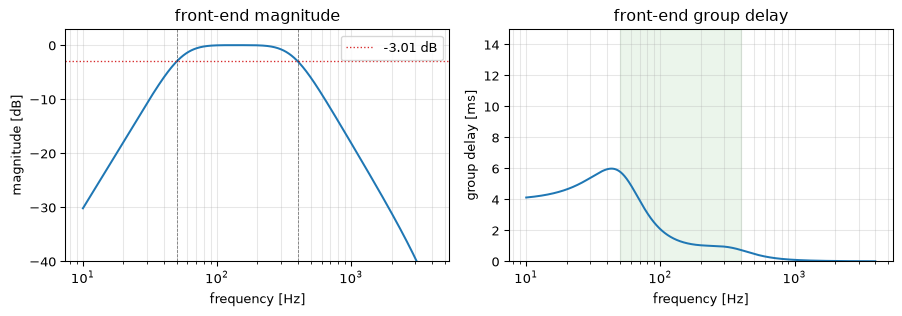
Speaking pitch lives between roughly 50 Hz (a low male voice) and 400 Hz (a high female or child voice). Everything below is rumble, mains hum, and handling noise; everything far above is vocal-tract detail the pitch estimator does not need. The front end is a second-order Butterworth bandpass over exactly that band, realised as two second-order sections (biquads). On the metal the coefficients are computed offline by a SciPy design script and pasted into the biquad cascade (this page keeps SciPy’s un-negated a1, a2; the workshop’s convention negates them); design_front_end is that script, kept importable.
Figure 1: The 50-400 Hz front end: two cascaded biquads, 40 dB/decade skirts on both sides. Left: magnitude response; the band edges sit at -3.01 dB by Butterworth construction, asserted below rather than read off the plot. Right: group delay; in the heart of the passband the filter delays the signal by a few milliseconds, worst near the low edge, negligible against the 64 ms analysis hop.
band-edge gains: -3.01 dB, -3.01 dB
From the archive: how the passband found its width
This system began as the author’s 2022 wearable prototype (a TinyPico ESP32 with an SPH0645 I2S MEMS microphone), and the front end carries its design history in its own source: the C header keeps three generations of coefficient sets as comments, a 40-1000 Hz band, then 40-500, then the 50-400 that shipped, each with its offline-computed SOS coefficients. The band narrowed as the project learned what the later stages actually needed: the cepstrum wants harmonic structure, not bandwidth, and everything admitted above the pitch band is noise the detector must then reject. The project log also records the class being renamed from pitch detector to pitch estimator midway: the arc’s founding distinction (is the quantity present, versus what is its value), discovered independently by a build that needed both answers at once.
The periodogram, averaged the streaming way
The spectral engine is the arc’s standard one: 2048-sample frames at 16 kHz (128 ms, more than six periods of even a 50 Hz voice, so the harmonic ripple the next section reads is well formed), Hamming-windowed (Harris 1978), DC removed per frame, 50% overlap, one-sided periodogram with the factor-of-two interior-bin convention the PSD page established (DC and Nyquist appear once in the double-sided spectrum, every other bin twice; test_vpe.py pins Parseval, sum(P) == sum(x**2), at 1e-10).
Instead of Welch’s fixed block average (Welch 1967), the streaming implementation smooths exponentially: \(\hat{P}_k = \alpha \hat{P}_{k-1} + (1-\alpha) P_k\) per frame. That is a scalar recursive estimator per bin, and the recursive-estimation page already priced it: an EMA with weight \(\alpha\) on the old value has the variance of a plain average over \((1+\alpha)/(1-\alpha)\) frames, so the hardware default \(\alpha = 0.1\) buys only a light touch (about 1.2 frames’ worth) and leaves the real averaging to the overlap; cranking \(\alpha\) toward 1 trades tracking speed for variance exactly as that page’s floor formula says. It is the same fast-attack knob the VAD will reuse below.
Cepstral pitch: read the quefrency axis the right way around
A voiced frame has a log-spectrum that is periodic in frequency: harmonics at \(f_0, 2f_0, 3f_0, \ldots\) ripple the log-periodogram with period \(f_0\). The cepstrum (Noll 1967) takes one more Fourier transform to find that ripple:
and a ripple with period \(f_0\) in frequency lands at quefrency\(q = f_s / f_0\) samples. Quefrency is time-like: it counts samples of period, not cycles of frequency. Two conventions follow, and both are load-bearing enough that the module docstring states them and the tests pin them:
a cepstral peak at index \(q\) means \(f_0 = f_s / q\), not \(q \cdot \Delta f\);
the search window for a 50-400 Hz pitch band is \(q \in [f_s/400,\; f_s/50] = [40, 320]\) at 16 kHz: higher pitch means smaller quefrency, so the window bounds flip relative to a frequency search.
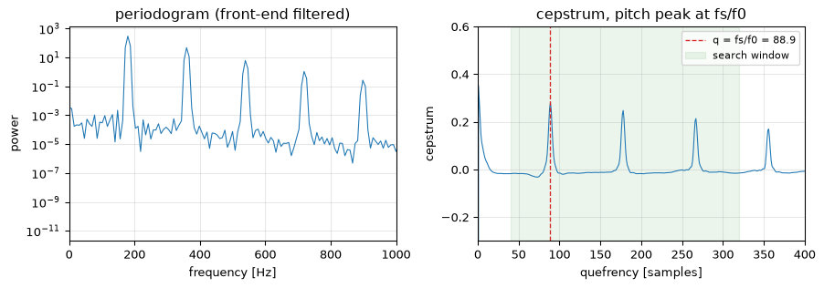
Two practical refinements complete the readout. The quefrency grid’s pitch resolution is \(f_0^2/f_s\) (differentiate \(f_0 = f_s/q\): one quefrency sample moves the pitch by \(f_s/q^2 = f_0^2/f_s\), so 5.6 Hz at 300 Hz and 16 kHz, worse the higher the pitch), so a three-point parabolic fit interpolates below the grid. And the cepstrum of real voiced speech peaks at \(q_0\)and its rahmonics \(2q_0, 3q_0, \ldots\); window leakage can push a rahmonic a hair above the fundamental, which would halve the reported pitch, so the reader walks down the rahmonic ladder when a comparable peak sits at half the winning quefrency (the octave-error guard every practical pitch tracker carries in some form (Mauch and Dixon 2014)).
The test signal in every figure on this page is the same synthetic vowel: harmonics of \(f_0\) at \(1/n\) amplitudes up to 4 kHz, fixed phases, plus white noise 40 dB down. That is a deliberately generous stand-in for voiced speech (the honest-limits section below discounts the margins it produces), but it has the one property ground truth requires: its \(f_0\) is exact.
Figure 2: The estimation chain on one voiced frame (synthetic vowel, f0 = 180 Hz, harmonics through 4 kHz, front-end filtered). Left: the one-sided periodogram; the front end has removed everything outside the pitch band, and the in-band harmonics at 180 and 360 Hz stand alone. Right: the cepstrum of the same frame; the pitch peak stands at quefrency q = fs/f0 = 88.9 samples (marked), with its rahmonic at 2q. The full readout recovers f0 within 1%, asserted below.
true f0: 180.0 Hz, estimated: 180.0 Hz
The ground-truth battery in test_vpe.py runs this recovery across the speaking range (100 to 300 Hz, with and without the front end, on and off the quefrency grid) and requires 2% or better everywhere; the same test doubles as the reference specification for the embedded implementation.
Why the cepstrum and not autocorrelation?
The pitch-detection page compares the families honestly; this system’s reasons are architectural. The cepstrum reuses the FFT machinery the periodogram already paid for (a second transform of the log-spectrum, and on a real even sequence at that, so the same real-FFT kernel serves), it separates excitation from vocal-tract envelope so the MFCC front end comes almost free later, and its peak location is immune to the formant-dominated spectral tilts that bias naive spectral peak picking. What it costs is the log’s noise sensitivity, which is exactly why the periodogram is floored and averaged before the log ever runs.
The detection chain: knowing when to say nothing
An estimator that always answers is a liability in this application: silence, breath, and unvoiced consonants have no \(f_0\), and a therapy display flashing random pitches during pauses is worse than useless. Deciding whether there is a pitch is a detection problem, and the detection-theory page’s machinery applies verbatim. The system fuses two features, one from each domain the pipeline already computes (Drugman et al. 2018):
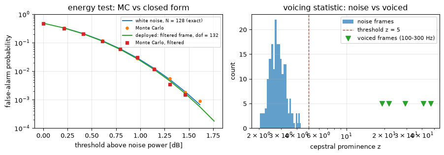
Energy against an adaptive threshold. The frame’s average power is the test statistic. Its distribution under noise is not guessed at: for \(N\) independent white-noise samples, \(N \bar{x^2} / \sigma^2 \sim \chi^2_N\), so a threshold’s false-alarm rate has a closed form. The catch, and the kind of detail this arc exists to keep honest, is that the VAD sees the frame after the 50-400 Hz front end, and filtered noise is no longer 2048 independent samples: the front end’s Welch-Satterthwaite equivalent bandwidth, \(B_{\mathrm{eq}} = \bigl(\int |H|^2 \mathrm{d}f\bigr)^2 / \int |H|^4 \mathrm{d}f = 516\) Hz, gives the deployed statistic an effective \(2 B_{\mathrm{eq}} T \approx 132\) degrees of freedom, four times more spread than the raw sample count suggests. A threshold 1 dB above the noise power is crossed by about 2% of noise-only frames (one every few seconds at the 64 ms hop), and comfortable margin starts near 2 dB; the figure below measures exactly this, Monte Carlo against the \(\chi^2_{132}\) tail. The threshold itself adapts: two trackers with fast-attack, slow-decay asymmetry follow the noise floor (attack downward) and the speech peaks (attack upward), and the threshold sits a fixed fraction \(\beta\) of the tracked dynamic range above the floor. That is the CFAR idea in miniature: estimate the local noise level, place the threshold relative to it, keep the false-alarm behaviour stable while the environment moves (Rohling 1983). What the simple tracker gives up against a true CFAR is the calibrated false-alarm rate; what it gains is two state variables and no window of reference cells. Two more of its time constants deserve price tags: the trackers’ relaxation weight (0.9999 per hop) means they forget over \(10^4\) hops, roughly ten minutes, deliberately session-scale memory, so a newly raised noise floor (a fan switching on) leans on the threshold for minutes; and until the first loud speech arrives, floor and ceiling both hug the noise level, the threshold sits essentially at the noise power, and the energy gate passes about half of all noise frames. At startup, silence rejection rests almost entirely on the second feature, which is the deeper reason the two are AND-gated.
Cepstral prominence. Energy alone cannot tell voiced speech from a slammed door. The cepstrum can: voicing means a peak in the pitch-band quefrency window, so the second feature is that peak’s height above the surrounding cepstral samples, in robust units (median and MAD, the outlier-detection page’s toolkit pointed the other way): a z-score for voicing. Under noise the floored cepstrum’s samples are approximately Gaussian with variance \(\pi^2 / (6 N_{\mathrm{fft}})\) (the log-periodogram’s bins are log-exponential with variance \(\pi^2/6\), and the IDFT averages them; tested by Monte Carlo), so the maximum of the roughly 280 samples in the search window sits where extreme-value behaviour puts the maximum of \(M\) Gaussians, near \(\sqrt{2 \ln M} = \sqrt{2 \ln 280} \approx 3.4\) (the same \(\sqrt{2 \ln N}\) that sets the wavelet page’s universal threshold (Donoho and Johnstone 1994)), and essentially never reaches the default threshold of 5. Voiced frames clear it several times over.
Show the code
rng = np.random.default_rng(5)n_small, n_mc =128, 20000powers = np.mean(rng.normal(size=(n_mc, n_small)) **2, axis=1)thresholds = np.linspace(1.05, 1.45, 9)p_mc = [(powers > t).mean() for t in thresholds]p_cf = chi2.sf(n_small * thresholds, df=n_small)# the DEPLOYED statistic: frame power after the 50-400 Hz front endf_bw = np.linspace(0, FS /2, 100001)_, h_bw = signal.sosfreqz(sos, worN=f_bw, fs=FS)S_bw = np.abs(h_bw) **2b_eq = np.trapezoid(S_bw, f_bw) **2/ np.trapezoid(S_bw **2, f_bw)dof =2* b_eq * NFFT / FSxf = signal.sosfilt(sos, rng.normal(size=2000* NFFT))p_filt = np.mean(xf.reshape(-1, NFFT) **2, axis=1)thr_f = np.linspace(1.0, 1.5, 11)pf_mc = [(p_filt > t * p_filt.mean()).mean() for t in thr_f]pf_cf = chi2.sf(dof * thr_f, df=dof)fig, axes = plt.subplots(1, 2, figsize=(9.5, 3.4))axes[0].semilogy(10* np.log10(thresholds), p_cf, 'C0-', label=f'white noise, N = {n_small} (exact)')axes[0].semilogy(10* np.log10(thresholds), p_mc, 'C1o', ms=4, label='Monte Carlo')axes[0].semilogy(10* np.log10(thr_f), pf_cf, 'C2-', label=f'deployed: filtered frame, dof = {dof:.0f}')axes[0].semilogy(10* np.log10(thr_f), pf_mc, 'C3s', ms=4, label='Monte Carlo, filtered')axes[0].set_ylim(1e-4, 1)axes[0].set_xlabel('threshold above noise power [dB]')axes[0].set_ylabel('false-alarm probability')axes[0].set_title('energy test: MC vs closed form'); axes[0].legend(fontsize=7)z_noise = []for _ inrange(200): p_n = one_sided_periodogram(rng.normal(size=NFFT), win) z_noise.append(cepstral_prominence(power_cepstrum(p_n, NFFT), FS))z_noise = np.array(z_noise)z_voiced = []f0s_demo = [100, 150, 200, 250, 300]for f0 in f0s_demo: xv = signal.sosfilt(sos, voiced(float(f0))) p_v = one_sided_periodogram(xv[-NFFT:], win) z_voiced.append(cepstral_prominence(power_cepstrum(p_v, NFFT), FS))axes[1].hist(z_noise, bins=25, alpha=0.7, label='noise frames')axes[1].axvline(5, color='C3', ls='--', lw=1, label='threshold z = 5')axes[1].plot(z_voiced, np.full(len(z_voiced), 5.0), 'C2v', ms=8, label='voiced frames (100-300 Hz)')axes[1].set_xscale('log')axes[1].set_xlabel('cepstral prominence z'); axes[1].set_ylabel('count')axes[1].set_title('voicing statistic: noise vs voiced'); axes[1].legend(fontsize=8)for ax in axes: ax.grid(True, alpha=0.3)fig.tight_layout(); plt.show()assert np.max(np.abs(np.array(p_mc) - p_cf)) <0.01assert np.max(np.abs(np.array(pf_mc) - pf_cf)) <0.02# deployed statisticprint(f"front-end B_eq = {b_eq:.0f} Hz -> effective dof = {dof:.0f}; "f"P_FA at 1 dB: {float(np.interp(10**0.1, thr_f, pf_cf)):.3f}")assert120< dof <145print(f"noise prominence: mean {z_noise.mean():.2f}, max {z_noise.max():.2f}; "f"voiced minimum {min(z_voiced):.1f}")assert z_noise.max() <5.0# the caption's exact claimassertmin(z_voiced) >2.5* z_noise.max() # separation from the noise maximumassertmin(z_voiced) >3*5.0# comfortably above the threshold
Figure 3: Both detection features, calibrated for the statistic the system actually computes. Left: false-alarm rate of the energy test versus threshold. The upper pair is the white-noise special case (20000 frames of N = 128 independent samples, Monte Carlo dots against the exact chi-square tail). The lower pair is the deployed statistic: 2000 front-end-filtered 2048-sample frames, whose effective degrees of freedom collapse to 2 B_eq T = 132; the dots follow the chi-square-132 tail, and both agreements are asserted below, the arc’s standing rule for detection statistics. Right: the voicing statistic; the cepstral prominence of 200 noise frames (histogram) never reaches the threshold at z = 5 (asserted), while voiced frames across the pitch range (markers) clear both the threshold and the largest noise excursion several-fold; the separation is asserted, not eyeballed.
front-end B_eq = 516 Hz -> effective dof = 132; P_FA at 1 dB: 0.024
noise prominence: mean 2.91, max 4.32; voiced minimum 19.2
The two features are AND-gated: energy says something is happening, prominence says it is periodic in the pitch band. Each covers the other’s blind spot (steady tonal interference can fool prominence but not the adaptive energy floor it raises; a door slam fools energy but not prominence), which is the modest, classical version of the feature-fusion idea that carries modern VAD design (Drugman et al. 2018).
Robustness: the Hampel gate on the pitch track
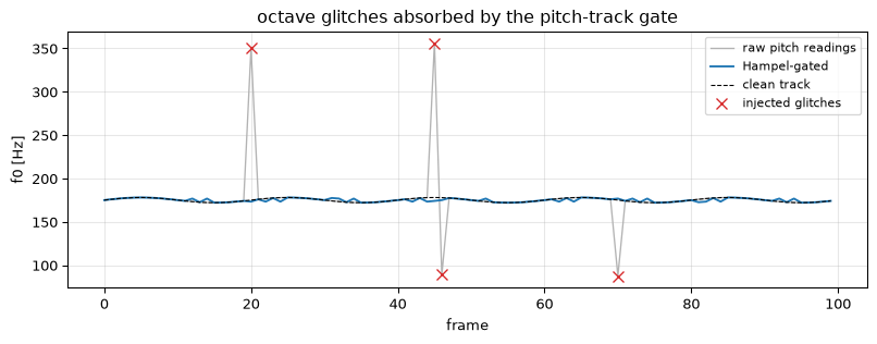
Even a gated estimator emits the occasional wild frame: an octave slip the rahmonic guard did not catch, a consonant transient, a breath. On a pitch track these are textbook impulsive outliers, and the outlier-detection page’s answer applies unchanged: a Hampel gate, eleven frames of memory, that replaces any reading more than \(k\) MADs from the window median by the median itself. Legitimate pitch movement (vibrato, intonation) has a healthy MAD and passes untouched; a lone octave jump is dozens of MADs out and is absorbed. The raw reading still enters the window, so a sustained change (a genuinely new pitch) works its way into the median within half a window rather than being suppressed forever.
Figure 4: The Hampel gate on a synthetic pitch track: 175 Hz with slow vibrato, plus four injected octave glitches (doubled or halved readings, marked). The raw track (grey) jumps by up to 175 Hz; the gated track (colour) stays within a few hertz of the clean track everywhere, asserted below. The gate costs eleven floats of state, which is why the same idea fits on the microcontroller.
max |error|: raw 178.0 Hz, gated 4.6 Hz
A gate like this is what separates a pitch readout that jumps an octave on a single bad frame from one steady enough to act on, which for a therapy display is the whole product; the median/MAD statistic it runs on is the same one the outlier-detection page develops in streaming form, at the same eleven-sample window size.
The whole machine, streaming
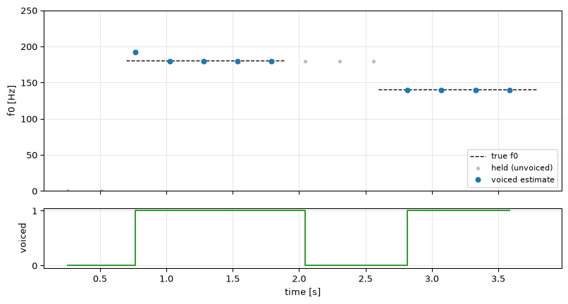
VoicePitchEstimator wires the stages together exactly as the embedded code does: consume a sample buffer, run the front end statefully across buffer boundaries, hop through 50%-overlapped frames, update the averaged periodogram, read the cepstral pitch, update the trackers, decide, gate, smooth. The pitch output holds through unvoiced stretches rather than decaying: the estimate is conditional on voicing, and the voiced flag, not a stale number, is what says whether to believe it.
Figure 5: A four-segment synthetic session through the full streaming estimator: noise, 1.2 s of voiced 180 Hz, noise, 1.2 s of voiced 140 Hz, processed in 4096-sample buffers as the hardware would. Top: the estimated track (colour where the VAD declares voicing, grey hold elsewhere) against truth (dashed). Bottom: the voiced flag. The estimate settles within 2% of truth in the second half of each voiced segment and the VAD stays quiet in both noise segments, all asserted below.
Honest limits: what classical buys, and where it stops
The pipeline above costs, per 128 ms frame, two 2048-point real FFTs, one biquad cascade pass, and a handful of scalar updates: well under a million cycles, a few percent of a 240 MHz microcontroller, with about 40 kB of working memory (the embedded page prices it stage by stage). It needs no training data, its failure modes are analysable (every threshold on this page came with a distribution), and each design number above was defended by a measurement or a closed form.
What the classical pipeline does not buy:
Adverse acoustics. The energy calibration assumed the noise entering the front end is broadly white (the equivalent-bandwidth correction above handles the front end itself, but not a coloured world); babble, reverberation, and competing speakers violate that, and the cepstral peak degrades gracefully but genuinely. Deep-learning estimators trained on exactly such data (CREPE (Kim et al. 2018), SPICE and successors) hold accuracy in conditions where any single-frame classical reader fails; probabilistic classical trackers (pYIN (Mauch and Dixon 2014)) close part of the gap by spreading the decision over time, at the price of Viterbi-style latency this real-time budget resists.
Irregular voicing. Creak, fry, and the breathy phonation that is precisely characteristic of Parkinsonian speech weaken the harmonic ripple the cepstrum reads. That is an uncomfortable, honest fact for this application: the population the device targets is the one that stresses the estimator most, and a serious deployment would validate against pathological-speech corpora, not synthetic vowels.
Octave ambiguity is managed, not solved. The rahmonic guard and the Hampel gate handle the common slips; a determined half-period voice (strong even harmonics, weak fundamental) can still fool a frame-local reader, which is why heavyweight trackers integrate over time.
The trade this system makes is the microcontroller trade: transparency, testability, and a cycle budget three orders of magnitude below a neural estimator, in exchange for robustness margins that a data-driven method wins in hostile conditions. Knowing which side of that trade an application sits on is the engineering decision; this page’s contribution is that every term of it is now measurable.
Going further
The MFCC door. The cepstrum computed here is one liftering step away from the MFCC page’s features: the low-quefrency half this page discards as “vocal tract” is exactly what speech recognition keeps. One pipeline, two applications, split at a quefrency.
A principled CFAR VAD. The min/max trackers work, but the detection-theory page’s cell-averaging CFAR would make the false-alarm rate a design constant rather than an emergent property; the cost is a window of noise reference frames and the care to exclude speech from it.
Time integration. Everything on this page is frame-local plus light smoothing. The next rung is a proper hidden-state model over frames: pitch continuity as a transition prior, voicing as a hidden switch (pYIN’s HMM (Mauch and Dixon 2014), or the model-based-filtering page’s Kalman machinery with a voicing gate).
The hardware. The embedded companion walks the ESP32 implementation this design shipped on: I2S microphone capture, the FreeRTOS task and mutex structure, the fixed-point-free float budget, and what would change on a NUCLEO-F446RE.
Donoho, David L., and Iain M. Johnstone. 1994. “Ideal Spatial Adaptation by Wavelet Shrinkage.”Biometrika 81 (3): 425–55.
Drugman, Thomas, Goeric Huybrechts, Viacheslav Klimkov, and Alexis Moinet. 2018. “Traditional Machine Learning for Pitch Detection.”IEEE Signal Processing Letters 25 (11): 1745–49. https://doi.org/10.1109/LSP.2018.2874155.
Harris, Fredric J. 1978. “On the Use of Windows for Harmonic Analysis with the Discrete Fourier Transform.”Proceedings of the IEEE 66 (1): 51–83.
Kim, Jong Wook, Justin Salamon, Peter Li, and Juan Pablo Bello. 2018. “CREPE: A Convolutional Representation for Pitch Estimation.” In Proceedings of the IEEE International Conference on Acoustics, Speech and Signal Processing (ICASSP), 161–65. https://doi.org/10.1109/ICASSP.2018.8461329.
Mauch, Matthias, and Simon Dixon. 2014. “PYIN: A Fundamental Frequency Estimator Using Probabilistic Threshold Distributions.”Proceedings of the IEEE International Conference on Acoustics, Speech and Signal Processing (ICASSP), 659–63. https://doi.org/10.1109/ICASSP.2014.6853678.
Noll, A. Michael. 1967. “Cepstrum Pitch Determination.”The Journal of the Acoustical Society of America 41 (2): 293–309. https://doi.org/10.1121/1.1910339.
Rohling, Hermann. 1983. “Radar CFAR Thresholding in Clutter and Multiple Target Situations.”IEEE Transactions on Aerospace and Electronic Systems AES-19 (4): 608–21. https://doi.org/10.1109/TAES.1983.309350.
Welch, Peter D. 1967. “The Use of Fast Fourier Transform for the Estimation of Power Spectra: A Method Based on Time Averaging over Short, Modified Periodograms.”IEEE Transactions on Audio and Electroacoustics 15 (2): 70–73.
Source Code
---title: "A Voice Pitch Estimator"subtitle: "The arc in one system: bandpass front end, periodogram, cepstral pitch, and a voicing decision, running on a microcontroller"description-meta: "One system end to end: bandpass front end, periodogram, cepstral pitch estimate and a voicing decision, tracking a speaking voice."bibliography: ../../references.bib---Every page of the [estimation & detection arc](../estimation-and-detection.qmd) so far studied one idea at a time: an estimator here, a detector there, a robustness trick in a third place. This capstone puts them in one machine. The task: track the fundamental frequency of a speaking voice, 50 to 400 Hz, in real time, on a low-power microcontroller, and know when to keep quiet because nobody is speaking. The application that motivated it is speech therapy for Parkinson's disease: a large fraction of people with Parkinson's develop reduced loudness and a monotone voice, intelligibility improves when they train louder speech at a controlled pitch, and a wearable pitch monitor is the feedback such training wants ([Parkinson's Foundation](https://www.parkinson.org/library/fact-sheets/speech-therapy), [Radboudumc Voice Trainer](https://www.radboudumc.nl/en/afdelingen/revalidatie/voice-trainer/voice-trainer)).The system is a classical pipeline, deliberately: bandpass front end, averaged periodogram, cepstral pitch readout, and a two-feature voice activity detector, with a Hampel gate guarding the pitch track. Each stage is a page of this arc doing its job in a running system, and the embedded companion is not an afterthought here: the hardware implementation (an ESP32 with an I2S MEMS microphone) is where this design comes from, the one piece of the arc where the metal predates the page. The [embedded page](embedded.qmd) walks the real-time architecture; this page builds the estimator and shows that every design number in it can be defended.::: {.callout-note title="Prerequisites"}Part of the [estimation & detection arc](../estimation-and-detection.qmd); the overview gives the reading order.The chain runs through most of the arc: [PSD estimation](../psd-estimation/index.qmd) for the periodogram and its conventions, [pitch detection](../pitch-detection/index.qmd) for cepstrum-versus-autocorrelation (this page commits to the cepstrum and does not re-fight that comparison), [detection theory](../detection-theory/index.qmd) for thresholds and false alarms, [outlier detection](../outlier-detection/index.qmd) for the Hampel filter, [recursive estimation](../recursive-estimation/index.qmd) for the exponential-forgetting variance floor behind the streaming periodogram and the VAD's trackers, and [statistical features](../statistical-features/index.qmd) for the VAD's feature vocabulary.:::::: {.callout-tip title="Code"}The implementation is [`vpe.py`](vpe.py). Save [`test_vpe.py`](test_vpe.py) beside it and `pytest test_vpe.py` runs the checks on it.:::```{python}#| echo: falseimport numpy as npimport matplotlib.pyplot as pltfrom scipy import signalfrom scipy.stats import chi2from vpe import (VoicePitchEstimator, HampelGate, cepstral_pitch, cepstral_prominence, design_front_end, frame_power, one_sided_periodogram, power_cepstrum)FS, NFFT =16000.0, 2048def voiced(f0, dur=0.5, fs=FS, n_harm=None, noise=0.01, seed=0): rng = np.random.default_rng(seed) t = np.arange(int(fs * dur)) / fsif n_harm isNone: n_harm =int(4000// f0) x =sum((1.0/ n) * np.cos(2* np.pi * n * f0 * t +0.7* n)for n inrange(1, n_harm +1))return x + noise * rng.normal(size=x.size)```<hr>## The estimation chain### A front end that knows what it is looking forSpeaking pitch lives between roughly 50 Hz (a low male voice) and 400 Hz (a high female or child voice). Everything below is rumble, mains hum, and handling noise; everything far above is vocal-tract detail the pitch estimator does not need. The front end is a second-order Butterworth bandpass over exactly that band, realised as two [second-order sections](../../basics/09-biquad/index.qmd) (biquads). On the metal the coefficients are computed offline by a SciPy design script and pasted into the biquad cascade (this page keeps SciPy's un-negated `a1`, `a2`; [the workshop's convention](../../basics/09-biquad/embedded.qmd#negated-coefficients) negates them); `design_front_end` is that script, kept importable.```{python}#| label: fig-front-end#| fig-cap: "The 50-400 Hz front end: two cascaded biquads, 40 dB/decade skirts on both sides. Left: magnitude response; the band edges sit at -3.01 dB by Butterworth construction, asserted below rather than read off the plot. Right: group delay; in the heart of the passband the filter delays the signal by a few milliseconds, worst near the low edge, negligible against the 64 ms analysis hop."sos = design_front_end(FS, (50.0, 400.0))f = np.logspace(np.log10(10), np.log10(4000), 2000)_, h = signal.sosfreqz(sos, worN=f, fs=FS)b, a = signal.sos2tf(sos)w_gd, gd = signal.group_delay((b, a), w=f, fs=FS)fig, axes = plt.subplots(1, 2, figsize=(9.5, 3.4))axes[0].semilogx(f, 20* np.log10(np.abs(h) +1e-15))axes[0].axhline(-3.01, color='C3', ls=':', lw=1, label='-3.01 dB')for edge in (50, 400): axes[0].axvline(edge, color='k', ls='--', lw=0.6, alpha=0.5)axes[0].set_ylim(-40, 3)axes[0].set_xlabel('frequency [Hz]'); axes[0].set_ylabel('magnitude [dB]')axes[0].set_title('front-end magnitude'); axes[0].legend()axes[1].semilogx(f, gd *1000/ FS)axes[1].axvspan(50, 400, color='green', alpha=0.08)axes[1].set_xlabel('frequency [Hz]'); axes[1].set_ylabel('group delay [ms]')axes[1].set_ylim(0, 15)axes[1].set_title('front-end group delay')for ax in axes: ax.grid(True, alpha=0.3, which='both')fig.tight_layout(); plt.show()_, h_edges = signal.sosfreqz(sos, worN=[50.0, 400.0], fs=FS)print("band-edge gains:", ", ".join(f"{20*np.log10(abs(g)):.2f} dB"for g in h_edges))assert np.allclose(np.abs(h_edges), 1/ np.sqrt(2), rtol=1e-3)gd_pass_ms = gd[(f >100) & (f <300)] *1000/ FSassert gd_pass_ms.max() <10```::: {.callout-note title="From the archive: how the passband found its width"}This system began as the author's 2022 wearable prototype (a TinyPico ESP32 with an SPH0645 I2S MEMS microphone), and the front end carries its design history in its own source: the C header keeps three generations of coefficient sets as comments, a 40-1000 Hz band, then 40-500, then the 50-400 that shipped, each with its offline-computed SOS coefficients. The band narrowed as the project learned what the later stages actually needed: the cepstrum wants harmonic *structure*, not bandwidth, and everything admitted above the pitch band is noise the detector must then reject. The project log also records the class being renamed from pitch *detector* to pitch *estimator* midway: the arc's founding distinction (is the quantity present, versus what is its value), discovered independently by a build that needed both answers at once.:::### The periodogram, averaged the streaming wayThe spectral engine is the arc's standard one: 2048-sample frames at 16 kHz (128 ms, more than six periods of even a 50 Hz voice, so the harmonic ripple the next section reads is well formed), Hamming-windowed [@harris1978use], DC removed per frame, 50% overlap, one-sided periodogram with the factor-of-two interior-bin convention the [PSD page](../psd-estimation/index.qmd) established (DC and Nyquist appear once in the double-sided spectrum, every other bin twice; `test_vpe.py` pins Parseval, `sum(P) == sum(x**2)`, at 1e-10).Instead of Welch's fixed block average [@welch1967use], the streaming implementation smooths exponentially: $\hat{P}_k = \alpha \hat{P}_{k-1} + (1-\alpha) P_k$ per frame. That is a scalar recursive estimator per bin, and the [recursive-estimation page](../recursive-estimation/index.qmd) already priced it: an EMA with weight $\alpha$ on the old value has the variance of a plain average over $(1+\alpha)/(1-\alpha)$ frames, so the hardware default $\alpha = 0.1$ buys only a light touch (about 1.2 frames' worth) and leaves the real averaging to the overlap; cranking $\alpha$ toward 1 trades tracking speed for variance exactly as that page's floor formula says. It is the same fast-attack knob the VAD will reuse below.### Cepstral pitch: read the quefrency axis the right way aroundA voiced frame has a log-spectrum that is *periodic in frequency*: harmonics at $f_0, 2f_0, 3f_0, \ldots$ ripple the log-periodogram with period $f_0$. The cepstrum [@noll1967cepstrum] takes one more Fourier transform to find that ripple:$$c[q] \;=\; \mathrm{IDFT}\bigl\{\, \log \hat{P}[k] \,\bigr\}[q],$$and a ripple with period $f_0$ in frequency lands at **quefrency** $q = f_s / f_0$ samples. Quefrency is time-like: it counts samples of period, not cycles of frequency. Two conventions follow, and both are load-bearing enough that the module docstring states them and the tests pin them:* a cepstral peak at index $q$ means $f_0 = f_s / q$, not $q \cdot \Delta f$;* the search window for a 50-400 Hz pitch band is $q \in [f_s/400,\; f_s/50] = [40, 320]$ at 16 kHz: *higher* pitch means *smaller* quefrency, so the window bounds flip relative to a frequency search.Two practical refinements complete the readout. The quefrency grid's pitch resolution is $f_0^2/f_s$ (differentiate $f_0 = f_s/q$: one quefrency sample moves the pitch by $f_s/q^2 = f_0^2/f_s$, so 5.6 Hz at 300 Hz and 16 kHz, worse the higher the pitch), so a three-point parabolic fit interpolates below the grid. And the cepstrum of real voiced speech peaks at $q_0$ *and* its rahmonics $2q_0, 3q_0, \ldots$; window leakage can push a rahmonic a hair above the fundamental, which would halve the reported pitch, so the reader walks down the rahmonic ladder when a comparable peak sits at half the winning quefrency (the octave-error guard every practical pitch tracker carries in some form [@mauch2014pyin]).The test signal in every figure on this page is the same synthetic vowel: harmonics of $f_0$ at $1/n$ amplitudes up to 4 kHz, fixed phases, plus white noise 40 dB down. That is a deliberately generous stand-in for voiced speech (the honest-limits section below discounts the margins it produces), but it has the one property ground truth requires: its $f_0$ is exact.```{python}#| label: fig-cepstrum#| fig-cap: "The estimation chain on one voiced frame (synthetic vowel, f0 = 180 Hz, harmonics through 4 kHz, front-end filtered). Left: the one-sided periodogram; the front end has removed everything outside the pitch band, and the in-band harmonics at 180 and 360 Hz stand alone. Right: the cepstrum of the same frame; the pitch peak stands at quefrency q = fs/f0 = 88.9 samples (marked), with its rahmonic at 2q. The full readout recovers f0 within 1%, asserted below."f0_true =180.0x = signal.sosfilt(sos, voiced(f0_true))win = np.hamming(NFFT)P = one_sided_periodogram(x[-NFFT:], win)c = power_cepstrum(P, NFFT)f0_est, peak = cepstral_pitch(c, FS)freqs = np.arange(P.size) * FS / NFFTqs = np.arange(c.size)fig, axes = plt.subplots(1, 2, figsize=(9.5, 3.4))axes[0].semilogy(freqs, P +1e-12, lw=0.8)axes[0].set_xlim(0, 1000)axes[0].set_xlabel('frequency [Hz]'); axes[0].set_ylabel('power')axes[0].set_title('periodogram (front-end filtered)')axes[1].plot(qs, c, lw=0.8)axes[1].axvline(FS / f0_true, color='C3', ls='--', lw=1, label=f'q = fs/f0 = {FS/f0_true:.1f}')axes[1].axvspan(40, 320, color='green', alpha=0.08, label='search window')axes[1].set_xlim(0, 400); axes[1].set_ylim(-0.3, max(0.6, 1.2* peak))axes[1].set_xlabel('quefrency [samples]'); axes[1].set_ylabel('cepstrum')axes[1].set_title('cepstrum, pitch peak at fs/f0'); axes[1].legend(fontsize=8)for ax in axes: ax.grid(True, alpha=0.3)fig.tight_layout(); plt.show()print(f"true f0: {f0_true} Hz, estimated: {f0_est:.1f} Hz")assertabs(f0_est / f0_true -1) <0.01```The ground-truth battery in `test_vpe.py` runs this recovery across the speaking range (100 to 300 Hz, with and without the front end, on and off the quefrency grid) and requires 2% or better everywhere; the same test doubles as the reference specification for the [embedded implementation](embedded.qmd).::: {.callout-tip title="Why the cepstrum and not autocorrelation?"}The [pitch-detection page](../pitch-detection/index.qmd) compares the families honestly; this system's reasons are architectural. The cepstrum reuses the FFT machinery the periodogram already paid for (a second transform of the log-spectrum, and on a real even sequence at that, so the same real-FFT kernel serves), it separates excitation from vocal-tract envelope so the [MFCC](../mfcc/index.qmd) front end comes almost free later, and its peak location is immune to the formant-dominated spectral tilts that bias naive spectral peak picking. What it costs is the log's noise sensitivity, which is exactly why the periodogram is floored and averaged before the log ever runs.:::<hr>## The detection chain: knowing when to say nothingAn estimator that always answers is a liability in this application: silence, breath, and unvoiced consonants have no $f_0$, and a therapy display flashing random pitches during pauses is worse than useless. Deciding *whether* there is a pitch is a detection problem, and the [detection-theory page's](../detection-theory/index.qmd) machinery applies verbatim. The system fuses two features, one from each domain the pipeline already computes [@drugman2018traditional]:**Energy against an adaptive threshold.** The frame's average power is the test statistic. Its distribution under noise is not guessed at: for $N$ independent white-noise samples, $N \bar{x^2} / \sigma^2 \sim \chi^2_N$, so a threshold's false-alarm rate has a closed form. The catch, and the kind of detail this arc exists to keep honest, is that the VAD sees the frame *after* the 50-400 Hz front end, and filtered noise is no longer 2048 independent samples: the front end's Welch-Satterthwaite equivalent bandwidth, $B_{\mathrm{eq}} = \bigl(\int |H|^2 \mathrm{d}f\bigr)^2 / \int |H|^4 \mathrm{d}f = 516$ Hz, gives the deployed statistic an effective $2 B_{\mathrm{eq}} T \approx 132$ degrees of freedom, four times more spread than the raw sample count suggests. A threshold 1 dB above the noise power is crossed by about 2% of noise-only frames (one every few seconds at the 64 ms hop), and comfortable margin starts near 2 dB; the figure below measures exactly this, Monte Carlo against the $\chi^2_{132}$ tail. The threshold itself adapts: two trackers with fast-attack, slow-decay asymmetry follow the noise floor (attack downward) and the speech peaks (attack upward), and the threshold sits a fixed fraction $\beta$ of the tracked dynamic range above the floor. That is the [CFAR idea](../detection-theory/index.qmd) in miniature: estimate the local noise level, place the threshold relative to it, keep the false-alarm behaviour stable while the environment moves [@rohling1983]. What the simple tracker gives up against a true CFAR is the *calibrated* false-alarm rate; what it gains is two state variables and no window of reference cells. Two more of its time constants deserve price tags: the trackers' relaxation weight (0.9999 per hop) means they forget over $10^4$ hops, roughly ten minutes, deliberately session-scale memory, so a newly raised noise floor (a fan switching on) leans on the threshold for minutes; and until the first loud speech arrives, floor and ceiling both hug the noise level, the threshold sits essentially *at* the noise power, and the energy gate passes about half of all noise frames. At startup, silence rejection rests almost entirely on the second feature, which is the deeper reason the two are AND-gated.**Cepstral prominence.** Energy alone cannot tell voiced speech from a slammed door. The cepstrum can: voicing means a *peak* in the pitch-band quefrency window, so the second feature is that peak's height above the surrounding cepstral samples, in robust units (median and MAD, the [outlier-detection page's](../outlier-detection/index.qmd) toolkit pointed the other way): a z-score for voicing. Under noise the floored cepstrum's samples are approximately Gaussian with variance $\pi^2 / (6 N_{\mathrm{fft}})$ (the log-periodogram's bins are log-exponential with variance $\pi^2/6$, and the IDFT averages them; tested by Monte Carlo), so the maximum of the roughly 280 samples in the search window sits where extreme-value behaviour puts the maximum of $M$ Gaussians, near $\sqrt{2 \ln M} = \sqrt{2 \ln 280} \approx 3.4$ (the same $\sqrt{2 \ln N}$ that sets the [wavelet page's](../wavelets/index.qmd) universal threshold [@donohojohnstone1994]), and essentially never reaches the default threshold of 5. Voiced frames clear it several times over.```{python}#| label: fig-vad#| fig-cap: "Both detection features, calibrated for the statistic the system actually computes. Left: false-alarm rate of the energy test versus threshold. The upper pair is the white-noise special case (20000 frames of N = 128 independent samples, Monte Carlo dots against the exact chi-square tail). The lower pair is the deployed statistic: 2000 front-end-filtered 2048-sample frames, whose effective degrees of freedom collapse to 2 B_eq T = 132; the dots follow the chi-square-132 tail, and both agreements are asserted below, the arc's standing rule for detection statistics. Right: the voicing statistic; the cepstral prominence of 200 noise frames (histogram) never reaches the threshold at z = 5 (asserted), while voiced frames across the pitch range (markers) clear both the threshold and the largest noise excursion several-fold; the separation is asserted, not eyeballed."rng = np.random.default_rng(5)n_small, n_mc =128, 20000powers = np.mean(rng.normal(size=(n_mc, n_small)) **2, axis=1)thresholds = np.linspace(1.05, 1.45, 9)p_mc = [(powers > t).mean() for t in thresholds]p_cf = chi2.sf(n_small * thresholds, df=n_small)# the DEPLOYED statistic: frame power after the 50-400 Hz front endf_bw = np.linspace(0, FS /2, 100001)_, h_bw = signal.sosfreqz(sos, worN=f_bw, fs=FS)S_bw = np.abs(h_bw) **2b_eq = np.trapezoid(S_bw, f_bw) **2/ np.trapezoid(S_bw **2, f_bw)dof =2* b_eq * NFFT / FSxf = signal.sosfilt(sos, rng.normal(size=2000* NFFT))p_filt = np.mean(xf.reshape(-1, NFFT) **2, axis=1)thr_f = np.linspace(1.0, 1.5, 11)pf_mc = [(p_filt > t * p_filt.mean()).mean() for t in thr_f]pf_cf = chi2.sf(dof * thr_f, df=dof)fig, axes = plt.subplots(1, 2, figsize=(9.5, 3.4))axes[0].semilogy(10* np.log10(thresholds), p_cf, 'C0-', label=f'white noise, N = {n_small} (exact)')axes[0].semilogy(10* np.log10(thresholds), p_mc, 'C1o', ms=4, label='Monte Carlo')axes[0].semilogy(10* np.log10(thr_f), pf_cf, 'C2-', label=f'deployed: filtered frame, dof = {dof:.0f}')axes[0].semilogy(10* np.log10(thr_f), pf_mc, 'C3s', ms=4, label='Monte Carlo, filtered')axes[0].set_ylim(1e-4, 1)axes[0].set_xlabel('threshold above noise power [dB]')axes[0].set_ylabel('false-alarm probability')axes[0].set_title('energy test: MC vs closed form'); axes[0].legend(fontsize=7)z_noise = []for _ inrange(200): p_n = one_sided_periodogram(rng.normal(size=NFFT), win) z_noise.append(cepstral_prominence(power_cepstrum(p_n, NFFT), FS))z_noise = np.array(z_noise)z_voiced = []f0s_demo = [100, 150, 200, 250, 300]for f0 in f0s_demo: xv = signal.sosfilt(sos, voiced(float(f0))) p_v = one_sided_periodogram(xv[-NFFT:], win) z_voiced.append(cepstral_prominence(power_cepstrum(p_v, NFFT), FS))axes[1].hist(z_noise, bins=25, alpha=0.7, label='noise frames')axes[1].axvline(5, color='C3', ls='--', lw=1, label='threshold z = 5')axes[1].plot(z_voiced, np.full(len(z_voiced), 5.0), 'C2v', ms=8, label='voiced frames (100-300 Hz)')axes[1].set_xscale('log')axes[1].set_xlabel('cepstral prominence z'); axes[1].set_ylabel('count')axes[1].set_title('voicing statistic: noise vs voiced'); axes[1].legend(fontsize=8)for ax in axes: ax.grid(True, alpha=0.3)fig.tight_layout(); plt.show()assert np.max(np.abs(np.array(p_mc) - p_cf)) <0.01assert np.max(np.abs(np.array(pf_mc) - pf_cf)) <0.02# deployed statisticprint(f"front-end B_eq = {b_eq:.0f} Hz -> effective dof = {dof:.0f}; "f"P_FA at 1 dB: {float(np.interp(10**0.1, thr_f, pf_cf)):.3f}")assert120< dof <145print(f"noise prominence: mean {z_noise.mean():.2f}, max {z_noise.max():.2f}; "f"voiced minimum {min(z_voiced):.1f}")assert z_noise.max() <5.0# the caption's exact claimassertmin(z_voiced) >2.5* z_noise.max() # separation from the noise maximumassertmin(z_voiced) >3*5.0# comfortably above the threshold```The two features are AND-gated: energy says *something* is happening, prominence says it is *periodic in the pitch band*. Each covers the other's blind spot (steady tonal interference can fool prominence but not the adaptive energy floor it raises; a door slam fools energy but not prominence), which is the modest, classical version of the feature-fusion idea that carries modern VAD design [@drugman2018traditional].<hr>## Robustness: the Hampel gate on the pitch trackEven a gated estimator emits the occasional wild frame: an octave slip the rahmonic guard did not catch, a consonant transient, a breath. On a pitch track these are textbook impulsive outliers, and the [outlier-detection page's](../outlier-detection/index.qmd) answer applies unchanged: a Hampel gate, eleven frames of memory, that replaces any reading more than $k$ MADs from the window median by the median itself. Legitimate pitch movement (vibrato, intonation) has a healthy MAD and passes untouched; a lone octave jump is dozens of MADs out and is absorbed. The raw reading still enters the window, so a *sustained* change (a genuinely new pitch) works its way into the median within half a window rather than being suppressed forever.```{python}#| label: fig-hampel#| fig-cap: "The Hampel gate on a synthetic pitch track: 175 Hz with slow vibrato, plus four injected octave glitches (doubled or halved readings, marked). The raw track (grey) jumps by up to 175 Hz; the gated track (colour) stays within a few hertz of the clean track everywhere, asserted below. The gate costs eleven floats of state, which is why the same idea fits on the microcontroller."n_frames =100t_fr = np.arange(n_frames)clean =175+3* np.sin(2* np.pi * t_fr /20)raw = clean.copy()glitch_at = [20, 45, 46, 70]raw[20] *=2; raw[45] *=2; raw[46] *=0.5; raw[70] *=0.5gate = HampelGate(window=11, k=4.0)gated = np.array([gate.process(v) for v in raw])fig, ax = plt.subplots(figsize=(8.5, 3.4))ax.plot(t_fr, raw, color='0.7', lw=1, label='raw pitch readings')ax.plot(t_fr, gated, 'C0', lw=1.4, label='Hampel-gated')ax.plot(t_fr, clean, 'k--', lw=0.8, label='clean track')ax.plot(glitch_at, raw[glitch_at], 'C3x', ms=8, label='injected glitches')ax.set_xlabel('frame'); ax.set_ylabel('f0 [Hz]')ax.set_title('octave glitches absorbed by the pitch-track gate')ax.legend(fontsize=8); ax.grid(True, alpha=0.3)fig.tight_layout(); plt.show()settled =slice(11, None) # once the window is fullerr_gated = np.abs(gated[settled] - clean[settled]).max()err_raw = np.abs(raw[settled] - clean[settled]).max()print(f"max |error|: raw {err_raw:.1f} Hz, gated {err_gated:.1f} Hz")assert err_raw >80assert err_gated <5```A gate like this is what separates a pitch readout that jumps an octave on a single bad frame from one steady enough to act on, which for a therapy display is the whole product; the median/MAD statistic it runs on is the same one the [outlier-detection page](../outlier-detection/index.qmd) develops in streaming form, at the same eleven-sample window size.<hr>## The whole machine, streaming`VoicePitchEstimator` wires the stages together exactly as the embedded code does: consume a sample buffer, run the front end statefully across buffer boundaries, hop through 50%-overlapped frames, update the averaged periodogram, read the cepstral pitch, update the trackers, decide, gate, smooth. The pitch output *holds* through unvoiced stretches rather than decaying: the estimate is conditional on voicing, and the voiced flag, not a stale number, is what says whether to believe it.```{python}#| label: fig-session#| fig-cap: "A four-segment synthetic session through the full streaming estimator: noise, 1.2 s of voiced 180 Hz, noise, 1.2 s of voiced 140 Hz, processed in 4096-sample buffers as the hardware would. Top: the estimated track (colour where the VAD declares voicing, grey hold elsewhere) against truth (dashed). Bottom: the voiced flag. The estimate settles within 2% of truth in the second half of each voiced segment and the VAD stays quiet in both noise segments, all asserted below."rng2 = np.random.default_rng(9)fs_i =int(FS)seg_noise =lambda n, s: 0.005* rng2.normal(size=int(n * fs_i))session = np.concatenate([ seg_noise(0.7, 1), voiced(180.0, dur=1.2, seed=2), seg_noise(0.7, 2), voiced(140.0, dur=1.2, seed=3),])truth = np.concatenate([ np.zeros(int(0.7* fs_i)), np.full(int(1.2* fs_i), 180.0), np.zeros(int(0.7* fs_i)), np.full(int(1.2* fs_i), 140.0),])est = VoicePitchEstimator()buf =4096times, f0s, flags = [], [], []for start inrange(0, session.size - buf +1, buf): voiced_flag, f0, _ = est.process(session[start: start + buf]) times.append((start + buf) / FS) f0s.append(f0); flags.append(voiced_flag)times, f0s, flags = np.array(times), np.array(f0s), np.array(flags)fig, axes = plt.subplots(2, 1, figsize=(8.5, 4.6), sharex=True, height_ratios=[3, 1])axes[0].plot(np.arange(truth.size) / FS, np.where(truth >0, truth, np.nan),'k--', lw=1, label='true f0')axes[0].plot(times[~flags], f0s[~flags], '.', color='0.75', ms=6, label='held (unvoiced)')axes[0].plot(times[flags], f0s[flags], 'C0o', ms=5, label='voiced estimate')axes[0].set_ylabel('f0 [Hz]'); axes[0].set_ylim(0, 250)axes[0].legend(fontsize=8, loc='lower right')axes[1].step(times, flags.astype(int), where='post', color='C2')axes[1].set_ylabel('voiced'); axes[1].set_xlabel('time [s]')axes[1].set_yticks([0, 1])for ax in axes: ax.grid(True, alpha=0.3)fig.tight_layout(); plt.show()def second_half(t0, t1):return (times > (t0 + t1) /2) & (times <= t1)for (t0, t1), f_true in [((0.7, 1.9), 180.0), ((2.6, 3.8), 140.0)]: sel = second_half(t0, t1) & flagsassert sel.any() err = np.abs(f0s[sel] / f_true -1).max()print(f"{f_true:.0f} Hz segment: settled error {100* err:.2f}%")assert err <0.02noise_sel = ((times >0.3) & (times <=0.7)) | ((times >2.3) & (times <=2.6))assertnot flags[noise_sel].any()```<hr>## Honest limits: what classical buys, and where it stopsThe pipeline above costs, per 128 ms frame, two 2048-point real FFTs, one biquad cascade pass, and a handful of scalar updates: well under a million cycles, a few percent of a 240 MHz microcontroller, with about 40 kB of working memory (the [embedded page](embedded.qmd) prices it stage by stage). It needs no training data, its failure modes are analysable (every threshold on this page came with a distribution), and each design number above was defended by a measurement or a closed form.What the classical pipeline does *not* buy:* **Adverse acoustics.** The energy calibration assumed the noise *entering* the front end is broadly white (the equivalent-bandwidth correction above handles the front end itself, but not a coloured world); babble, reverberation, and competing speakers violate that, and the cepstral peak degrades gracefully but genuinely. Deep-learning estimators trained on exactly such data (CREPE [@kim2018crepe], SPICE and successors) hold accuracy in conditions where any single-frame classical reader fails; probabilistic classical trackers (pYIN [@mauch2014pyin]) close part of the gap by spreading the decision over time, at the price of Viterbi-style latency this real-time budget resists.* **Irregular voicing.** Creak, fry, and the breathy phonation that is precisely characteristic of Parkinsonian speech weaken the harmonic ripple the cepstrum reads. That is an uncomfortable, honest fact for this application: the population the device targets is the one that stresses the estimator most, and a serious deployment would validate against pathological-speech corpora, not synthetic vowels.* **Octave ambiguity is managed, not solved.** The rahmonic guard and the Hampel gate handle the common slips; a determined half-period voice (strong even harmonics, weak fundamental) can still fool a frame-local reader, which is why heavyweight trackers integrate over time.The trade this system makes is the microcontroller trade: transparency, testability, and a cycle budget three orders of magnitude below a neural estimator, in exchange for robustness margins that a data-driven method wins in hostile conditions. Knowing which side of that trade an application sits on is the engineering decision; this page's contribution is that every term of it is now measurable.<hr>## Going further**The MFCC door.** The cepstrum computed here is one liftering step away from the [MFCC page's](../mfcc/index.qmd) features: the low-quefrency half this page discards as "vocal tract" is exactly what speech recognition keeps. One pipeline, two applications, split at a quefrency.**A principled CFAR VAD.** The min/max trackers work, but the [detection-theory page's](../detection-theory/index.qmd) cell-averaging CFAR would make the false-alarm rate a *design constant* rather than an emergent property; the cost is a window of noise reference frames and the care to exclude speech from it.**Time integration.** Everything on this page is frame-local plus light smoothing. The next rung is a proper hidden-state model over frames: pitch continuity as a transition prior, voicing as a hidden switch (pYIN's HMM [@mauch2014pyin], or the [model-based-filtering page's](../model-based-filtering/index.qmd) Kalman machinery with a voicing gate).**The hardware.** The [embedded companion](embedded.qmd) walks the ESP32 implementation this design shipped on: I2S microphone capture, the FreeRTOS task and mutex structure, the fixed-point-free float budget, and what would change on a NUCLEO-F446RE.**The whole arc.** The [estimation & detection overview](../estimation-and-detection.qmd) threads all eight pages in order and places this capstone in the ladder.## References::: {#refs}:::