A drift monitor riding the CFAR detector’s own block-energy stream, in integer arithmetic, on STM32F4 and ESP32-S3
The CFAR burst detector of the detection page holds its designed false-alarm rate on any board, at any gain setting, with no calibration constant anywhere in the chain, because the ratio it computes cancels the microphone sensitivity, the amplifier gain, and the noise level all at once.
That immunity is also a blind spot, and it is worth stating plainly: a detector engineered to be indifferent to the noise level cannot tell you when the noise level changes. The microphone port fills with dust, the preamp’s bias drifts with temperature, a cable develops a partial break, the enclosure gasket fails and the fan gets louder. The CFAR quietly re-learns each new floor within its reference window and carries on reporting bursts exactly as specified. Nothing is broken. Nothing is reported either, and for a device that is supposed to sit in a machine room for three years, the drift is the interesting signal.
This page adds the instrument that notices, on the stream the CFAR is already computing. It costs 276 bytes of state and a few tens of cycles per 8 ms block, needs no additional sampling, and its design numbers come from the main page. It is also the page where that theory stops being enough, twice, in ways worth the space.
How the integer pipeline is checked
The integer pipeline below is implemented in intcusum.py using only operations the C performs, including the truncating shifts, and test_intcusum.py pins its behaviour; the float reference is changedet.py. Save all three in one directory and pytest test_intcusum.py runs those checks: two of them compare the integer pipeline against the float one, so changedet.py has to be there too. Cycle counts are budgets from instruction counts, marked as such. The bench protocol at the end is what turns those budgets into measured figures, and the final section explains why on this particular detector that step is not optional.
The design, in numbers
Everything is inherited from the CFAR detector’s front end, which is the point: no new sampling, no new buffers, no new timing.
Sample rate\(f_s = 8\) kHz and block length\(M = 64\) samples, as on the CFAR page: 125 block energies per second, already being computed.
The statistic is \(\ln E\), the natural log of the block energy. A change in noise power is multiplicative; the log makes it additive, which is the form a CUSUM accumulates.
The energy is the CFAR’s own, taken one line early.energy_push computes the integer numerator \(N = M\sum x^2 - (\sum x)^2\) and then divides by \(M\) and casts to float. The drift monitor takes \(N\) itself, which keeps it in integers and costs nothing. This matters more than it looks: \(N\) removes the block mean, so it is exactly invariant to the ADC’s mid-rail pedestal. A raw sum of squares is not, and at mid-rail it is roughly 99.8% pedestal, which would leave a 1 dB drift moving the statistic by well under 1% of the CUSUM’s per-block slack. A monitor wired to the raw sum would be deaf to precisely the drift it exists to catch.
The in-control spread is known in closed form.\(\ln\) of a \(\chi^2_{M-1}\) variable has variance \(\psi'\!\left(\frac{M-1}{2}\right)\), so no calibration run is needed to know the noise on the statistic, only to know its mean. It is \(M-1\) and not \(M\) because the block mean was estimated from the block, the same degree of freedom the CFAR page spends on its own thresholds. The constant factor \(M\) in \(N\) is an additive constant in log space and is absorbed by the stored baseline, so it never has to be divided out.
What counts as a change: 1 dB. Chosen because the detection page measured that a one-decibel error in the assumed floor is exactly what turns a \(10^{-3}\) false-alarm rate into one in twenty. One decibel is the natural unit of “this matters”.
False-alarm budget: one per hour. A maintenance alert, not a per-block decision.
M, FS =64, 8000BPS = FS / M # blocks per secondSD =float(np.sqrt(polygamma(1, (M -1) /2))) # nats, exact; M-1, not Mdelta_1db = np.log(10**0.1) / SD # 1 dB, in sigma unitsprint(f"{BPS:.0f} blocks/s; log-energy sigma = {SD:.4f} nats "f"= {10* np.log10(np.e) * SD:.3f} dB")print(f"a 1 dB drift is {delta_1db:.2f} sigma of the block-to-block scatter\n")# Two-sided: design EACH arm for twice the target rate.target_h =3600* BPS *2k_d, h_d = design_cusum(delta_1db, target_h)print(f"k = {k_d:.4f}, h = {h_d:.4f} (each arm at ARL0 = {target_h:.0f} blocks)")print(f"\n{'drift':>7}{'delay [blocks]':>16}{'delay [ms]':>12}")for db in (0.5, 1.0, 2.0, 3.0): s = np.log(10** (db /10)) / SD a1 = arl_markov(k_d, h_d, s)print(f"{db:5.1f} dB {a1:16.1f}{a1 / BPS *1000:12.0f}")if db ==1.0:assert13< a1 <16, "the quoted ~14-block delay at 1 dB"assertabs(10* np.log10(np.e) * SD -0.780) <0.002assertabs(delta_1db -1.28) <0.01
125 blocks/s; log-energy sigma = 0.1796 nats = 0.780 dB
a 1 dB drift is 1.28 sigma of the block-to-block scatter

k = 0.6410, h = 9.3863  (each arm at ARL0 = 900000 blocks)

  drift   delay [blocks]   delay [ms]
  0.5 dB            111.3          891
  1.0 dB             15.3          122
  2.0 dB              5.5           44
  3.0 dB              3.5           28
A one-decibel drift is caught in about a tenth of a second while false alarms are an hour apart. That ratio, roughly \(3 \times 10^4\) between the two time scales, is the practical face of the main page’s logarithmic trade: moving from one false alarm per hour to one per day would cost about 30 ms more delay.
The one transcendental in the loop
The CUSUM is two adds and a compare. The logarithm is the expensive part, and on a Cortex-M4F logf from libm is roughly two orders of magnitude more work than everything else in the block combined. It is also completely unnecessary at this precision, because the answer only has to be small compared with the 0.178-nat scatter of the quantity being measured.
Take the exponent from the integer’s bit length and fit a cubic to the mantissa on \([0.5, 1)\):
\[\ln E = p \ln 2 + \ln m, \qquad E = m \cdot 2^{p}, \quad m \in [0.5, 1)\]
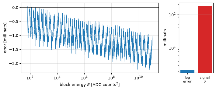
Figure 1: Error of the integer logarithm against the exact value, over the whole range 64 samples of a 12-bit ADC can produce (a few counts of noise up to full scale). The sawtooth is the cubic’s fit error repeating once per octave; the fuzz on it is Q12 truncation. The worst case is 2.2 millinats, which is 1.2% of the log-energy standard deviation drawn to scale on the right, so the approximation is invisible to the detector.
worst-case error 2.23 millinats = 1.239% of a log-energy sigma
Two details of that implementation are worth naming because both are places where an integer log goes quietly wrong.
It is not strictly monotone. Truncation in the Q12 Horner steps means adjacent energies occasionally produce a log that decreases by exactly one count, \(1/4096\) of a nat. That is a quarter of the polynomial’s own error and 0.14% of a sigma, so it is harmless here, but a routine that assumed monotonicity (a binary search, a sorted-order argument) would be wrong. The test pins the real property: monotone to within one count, never more.
\(\ln 0\) is a hardware state, not a hypothetical. A muted microphone, an unplugged input, or a DMA buffer read before the first conversion completes all deliver a block energy of exactly zero, and \(\ln 0\) has no representation. This workshop has met this exact hazard before, on the voice-pitch capstone’s cepstrum, and the fix has the same two halves: floor the argument, and saturate the accumulator, because they catch different failures.
INV_SD_Q8 =int(round(256.0/ SD))mu_demo = int_ln_q12(64*1000**2) # a plausible baselinez_if_unfloored = ((0- mu_demo) * INV_SD_Q8) >>12print(f"an unfloored ln(0) would push z to {z_if_unfloored /256:.0f} sigma "f"in one block")print(f"int16 Q8 holds {32767/256:.0f} sigma: one such block nearly fills "f"the accumulator")print(f"floored, ln(0) is treated as ln(1) = {int_ln_q12(0) /4096:.4f}")assert int_ln_q12(0) == int_ln_q12(1)assertabs(z_if_unfloored /256) >0.5* (32767/256), "genuinely close to full"
an unfloored ln(0) would push z to -100 sigma in one block
int16 Q8 holds 128 sigma: one such block nearly fills the accumulator
floored, ln(0) is treated as ln(1) = 0.0002
The floor turns a dead input into a large but sane downward deviation, which the lower CUSUM arm reports as what it is: the signal stopped. The saturating add is the backstop for everything the floor does not anticipate.
Fixed point is the boring part
It is tempting to expect trouble from Q8 arithmetic. There is none, and the reason is arithmetic rather than luck: the quantization step is \(1/256 \approx 0.004\) sigma, while the reference value \(k\) is 0.65 sigma, so the rounding is 0.6% of the smallest quantity in the recursion. Fed the same stream with the same design, the integer detector produces the same alarms at the same block indices as the float reference, which is what test_intcusum.py asserts rather than hopes.
Show the code
rng = np.random.default_rng(31)K_Q8, H_Q8 =int(round(k_d *256)), int(round(h_d *256))train = adc_block_energies(4000, 1000.0, rng)mu_q12 =int(round(np.mean([int_ln_q12(int(v)) for v in train])))mon = IntDriftMonitor(k_q8=K_Q8, h_q8=H_Q8, inv_sd_q8=INV_SD_Q8, mu_q12=mu_q12)for v in adc_block_energies(60000, 1000.0, rng): mon.push(int(v))print(f"K_Q8 = {K_Q8}, H_Q8 = {H_Q8}, INV_SD_Q8 = {INV_SD_Q8}")print(f"k quantized to {abs(K_Q8 /256- k_d) / k_d:.2%}, "f"h to {abs(H_Q8 /256- h_d) / h_d:.2%}")print(f"accumulator high-water mark over 8 minutes of quiet input: "f"{mon.peak} Q8 = {mon.peak /256:.1f} sigma "f"(int16 holds {32767/256:.0f})")assert mon.peak <32767//2, "int16 must not be marginal"
K_Q8 = 164, H_Q8 = 2403, INV_SD_Q8 = 1425
k quantized to 0.06%, h to 0.00%
accumulator high-water mark over 8 minutes of quiet input: 2168 Q8 = 8.5 sigma (int16 holds 128)
So the state is: two int16 arms, one int32 baseline, two int16 design constants, an int32 scale factor, two uint16 ring indices, and the ring itself. On a 32-bit target with natural alignment that is 276 bytes, of which the 128-entry int16 ring is 256; the ring is the only part that scales, but halving it to 64 entries is not free: it costs about a fifth of the false-alarm budget (measured below).
The firmware
The detector is pure arithmetic on a stream, so unlike the CFAR page there is nothing platform-specific here: the ADC setup, DMA, and block accumulation are already done by that page’s energy_push, on either default platform (NUCLEO-F446RE or ESP32-S3), and this code taps its accumulator. That is the whole argument for putting the drift monitor here rather than giving it its own sampling chain.
The tap needs one line of care, and it is the line where this design would most easily go wrong. energy_push ends by computing an int64_t numerator and then dividing by M and casting to float. The drift monitor wants the numerator, before the divide: it is an exact integer, it is what the \(\chi^2_{M-1}\) constants above describe, and because it has the block mean removed it is untouched by the ADC’s mid-rail pedestal. Handing over the float energy would force a cast back to integer; handing over the raw sumsq would be worse than useless, for the reason given in the design list. So energy_push gains one line:
/* Inside the CFAR page's energy_push(), the numerator already exists. Publish it; the divide and the float stay exactly as they were. */int64_t num =(int64_t)a->sumsq * M_BLOCK-(int64_t)a->sum *(int64_t)a->sum;*energy =(float)num /(float)M_BLOCK;/* CFAR, unchanged */*energy_n =(uint64_t)num;/* the drift monitor's */
That is the entire interface change: no new accumulator, no second pass over the samples, and nothing added to the per-sample path.
/* drift.c -- integer CUSUM drift monitor on a block-energy stream. * * Hooks onto the CFAR detector's energy_push(): whenever a block * completes, hand it the INTEGER energy numerator * N = M * sum(x^2) - (sum x)^2, * not the float energy and not the raw sum of squares. N has the * block mean removed, so it is exactly invariant to the ADC's * mid-rail pedestal, and it is chi-square with M-1 degrees of * freedom. No FPU, no libm, no division, no dynamic memory. */#include <stdint.h>#define REBASE_N 128/* power of two: the /N is a shift */#define REBASE_SHIFT 7#define Q8_MAX 32767/* ln(m) on [0.5,1), degree-3, coefficients in Q12 */#define LN_C3 3530#define LN_C2 (-11802)#define LN_C1 17202#define LN_C0 (-8929)#define LN2_Q12 2839/* round(ln(2) * 4096) */typedefstruct{int16_t k_q8, h_q8;/* design constants, sigma units */int32_t inv_sd_q8;/* round(256 / sd_nats) */int32_t mu_q12;/* baseline log-energy, Q12 nats */int16_t hi, lo;/* the two CUSUM arms, both >= 0 */int16_t hist[REBASE_N];/* recent log-energies, Q12 >> 4 */uint16_t head, filled;} drift_t;/* Natural log of a positive integer, Q12, integers only. */staticint32_t int_ln_q12(uint64_t e){int32_t t, p;uint32_t m_q15;if(e ==0u) e =1u;/* ln(0) is a real hardware state */ p =64- __builtin_clzll(e);/* e in [2^(p-1), 2^p) */ m_q15 =(p >=15)?(uint32_t)(e >>(p -15)):(uint32_t)(e <<(15- p)); t = LN_C3; t =((t *(int32_t)m_q15)>>15)+ LN_C2; t =((t *(int32_t)m_q15)>>15)+ LN_C1; t =((t *(int32_t)m_q15)>>15)+ LN_C0;return p * LN2_Q12 + t;}staticint16_t sat16(int32_t v){if(v <0)return0;/* the CUSUM floor at zero */if(v > Q8_MAX)return Q8_MAX;/* saturate; never wrap */return(int16_t)v;}void drift_init(drift_t *d,int16_t k_q8,int16_t h_q8,int32_t inv_sd_q8,int32_t mu_q12){uint16_t i; d->k_q8 = k_q8; d->h_q8 = h_q8; d->inv_sd_q8 = inv_sd_q8; d->mu_q12 = mu_q12; d->hi = d->lo =0; d->head = d->filled =0;for(i =0; i < REBASE_N; i++) d->hist[i]=0;}/* Returns +1 (floor rose), -1 (floor fell), or 0. Call once per block. */int drift_push(drift_t *d,uint64_t energy){int32_t ln_q12 = int_ln_q12(energy);int32_t z_q8, sum;int dir;uint16_t i; d->hist[d->head]=(int16_t)(ln_q12 >>4);/* Q8 nats: fits */ d->head =(uint16_t)((d->head +1u)&(REBASE_N -1u));if(d->filled < REBASE_N) d->filled++; z_q8 =((ln_q12 - d->mu_q12)* d->inv_sd_q8)>>12; d->hi = sat16((int32_t)d->hi + z_q8 - d->k_q8); d->lo = sat16((int32_t)d->lo - z_q8 - d->k_q8);if(d->hi < d->h_q8 && d->lo < d->h_q8)return0; dir =(d->hi >= d->h_q8)?+1:-1; d->hi = d->lo =0;/* Re-baseline from the ring, but ONLY once it lies entirely after * the change we just reported: otherwise the stale samples pull the * estimate back and the detector re-fires immediately. */if(d->filled >= REBASE_N){ sum =0;for(i =0; i < REBASE_N; i++) sum += d->hist[i]; d->mu_q12 =(sum >> REBASE_SHIFT)<<4;/* Q8 back to Q12 */ d->filled =0;/* refill before next */}return dir;}
The d->filled = 0 on the last line is the whole of the next section compressed into one statement, and it is the least obvious line in the file.
The baseline is where the difficulty actually lives
After a real drift, \(\mu_0\) is stale. Every subsequent block is genuinely far from it, so the statistic re-crosses the threshold immediately, and keeps doing so forever: a detector that reports the same change several times a second is worse than useless, because it buries the one report that mattered. The detector must adopt the new floor as normal, which means re-estimating \(\mu_0\) from recent data.
How much recent data is the design question, and it is not “as much as possible”.
Show the code
rng_r = np.random.default_rng(32)k_r, h_r = design_cusum(delta_1db, 2000.0)K_R, H_R =int(round(k_r *256)), int(round(h_r *256))n_pre, n_post, reps =400, 2500, 25train_r = adc_block_energies(4000, 1000.0, rng_r)mu_r =int(round(np.mean([int_ln_q12(int(v)) for v in train_r])))windows = (16, 32, 64, 128, 256, 512, 1024)rates = []for w in windows: total =0 r = np.random.default_rng(33)for _ inrange(reps): e = np.concatenate((adc_block_energies(n_pre, 1000.0, r), adc_block_energies(n_post, 1000.0*10** (1/20), r))) d = IntDriftMonitor(k_q8=K_R, h_q8=H_R, inv_sd_q8=INV_SD_Q8, mu_q12=mu_r, rebase_n=w)# count alarms once the window has had a chance to be clean total +=sum(1for i, _ in d.run(int(v) for v in e)if i >= n_pre +200) rates.append((n_post -200) * reps /max(total, 1))fig, ax = plt.subplots(figsize=(7.5, 3.6))ax.semilogx(windows, rates, 'C0-o', lw=1.4, ms=5, base=2)ax.axhline(1000, color='C2', ls=':', lw=1.2, label='design rate, two-sided (no drift)')ax.axvline(200, color='k', ls='--', lw=1, label='window longer than the time since the step')ax.set_xlabel('re-baselining window [blocks]')ax.set_ylabel('blocks per false alarm')ax.legend(fontsize=8); ax.grid(True, alpha=0.3, which='both')fig.tight_layout(); plt.show()for w, r_ inzip(windows, rates):print(f" {w:5d}-block window: 1 alarm per {r_:6.0f} blocks")best =int(np.argmax(rates))print(f"best: {windows[best]} blocks; worst-to-best penalty "f"{rates[best] / rates[-1]:.0f}x, "f"halving from {windows[best]} to {windows[best -1]} costs "f"{100* (1- rates[best -1] / rates[best]):.0f}%")assert rates[0] < rates[best], "a short window is too noisy"assert rates[-1] < rates[best], "an over-long window straddles the change"assert32<= windows[best] <=512, "the useful range"assert21< rates[best] / rates[-1] <28, "the caption's 24x asymmetry claim"assert0.16<1- rates[best -1] / rates[best] <0.28, \"the caption's 22% cost of halving the ring"
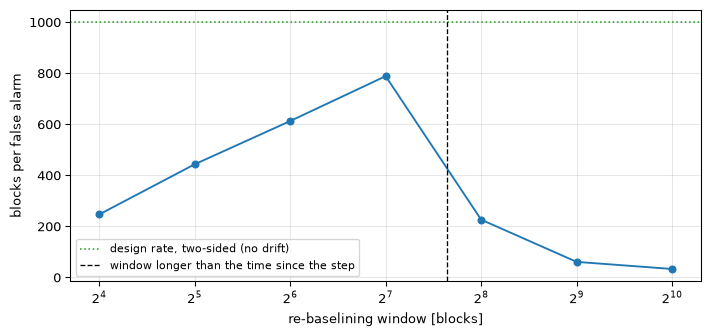
Figure 2: Alarm rate after a 1 dB step, against the length of the window used to re-estimate the baseline, measured on the integer detector at a threshold designed for one false alarm per 1000 blocks two-sided (a low threshold, so the experiment is affordable). Left of the dashed line the estimate is too noisy and its error costs false alarms; right of it the window is longer than the time elapsed since the step, so it averages data from both sides and lands between them. The curve is measured with the firmware’s filled = 0 policy in force, and that policy is what makes the right-hand fall-off so steep: a window the detector cannot refill with post-change blocks leaves the stale baseline in place for longer, so the two effects compound and the 1024-block window ends up 24x worse than the best one. The optimum is correspondingly sharp rather than a plateau: halving from 128 to 64 costs 22%, so the window length is a number to measure rather than to guess.
     16-block window: 1 alarm per    246 blocks
     32-block window: 1 alarm per    442 blocks
     64-block window: 1 alarm per    612 blocks
    128-block window: 1 alarm per    788 blocks
    256-block window: 1 alarm per    225 blocks
    512-block window: 1 alarm per     60 blocks
   1024-block window: 1 alarm per     32 blocks
best: 128 blocks; worst-to-best penalty 24x, halving from 128 to 64 costs 22%
Both ends of that curve are worth reading. A short window leaves an estimate with standard error \(\sigma/\sqrt{N}\), and since the CUSUM’s run length depends exponentially on its threshold, a small baseline error is expensive. A window longer than the interval between changes is worse, because it averages data from both sides of the step and lands between them, so the detector is permanently offset from both. The firmware’s answer is the filled = 0 line: after an alarm it refuses to re-baseline again until the ring holds only post-change blocks.
Where the design stops being trustworthy
Here is the part this page exists for, and it is not a caveat, it is the finding.
The whole design above rests on the block-energy log being close enough to Gaussian, which the main page checked and found true near the middle of the distribution. A threshold set for one false alarm per hour is not near the middle. At \(h \approx 9.4\) the run length is governed entirely by the tail of the increment distribution, and \(\ln \chi^2_{63}\) has a heavier left tail than a Gaussian of the same variance. The consequence compounds exponentially with the threshold:
Show the code
from scipy.stats import chi2, normz_tail = (np.log(chi2.ppf([0.5, 0.16, 0.023, 1.35e-3, 3.2e-5], M -1))- np.log(chi2.ppf(0.5, M -1))) / SDprint(f"{'Gaussian quantile':>18}{'log-energy z':>14}{'Gaussian z':>12}")for q, zt, zg inzip((0.5, 0.16, 0.023, 1.35e-3, 3.2e-5), z_tail, (0.0, -1.0, -2.0, -3.0, -4.0)):print(f"{q:18.5f}{zt:14.2f}{zg:12.2f}")assert z_tail[-1] <-4.0, "the left tail really is heavier"print(f"\nat the 3.2e-5 quantile the log-energy deviate is "f"{z_tail[-1] /-4.0:.2f}x the Gaussian one")
 Gaussian quantile   log-energy z   Gaussian z
           0.50000           0.00         0.00
           0.16000          -1.02        -1.00
           0.02300          -2.11        -2.00
           0.00135          -3.28        -3.00
           0.00003          -4.52        -4.00

at the 3.2e-5 quantile the log-energy deviate is 1.13x the Gaussian one
Fed into a CUSUM at a deep threshold, that heavier tail means the downward arm fires sooner than the design promised. Simulating the integer detector at the one-per-hour threshold measures 0.60 \(\pm\) 0.05 hours between false alarms against a 1.0 hour design (120 runs, none censored), and restoring the target needs \(h\) raised by about 0.3, to roughly 9.7, which measures 0.95 \(\pm\) 0.08 hours; 10.0 overshoots to 1.21 \(\pm\) 0.10. Those runs are not repeated at page-render time; what matters is not the specific correction but the rule it illustrates, which is the third time this arc has arrived at the same place:
A threshold for a rare event cannot be inherited from a distribution you only approximately believe. The Gaussian theory tells you which threshold to try. Only the stream tells you what it costs.
Budget and bench protocol
Per block, the drift monitor is one clz, three multiply-accumulates for the polynomial, one multiply for the standardization, and four adds with compares, plus a 128-entry summation on the rare blocks that alarm. Against the 64 multiply-accumulates the block energy already costs, it is noise.
Tier
Per block (estimated)
Per second at 125 blocks/s
Verdict
Cortex-M4F (NUCLEO-F446RE)
~40 cycles
~5 kcycles
0.003% of 180 MHz
ESP32-S3 (Xtensa LX7)
~50 cycles
~6 kcycles
negligible
Cortex-M0+ (no clz penalty, no divide)
~90 cycles
~11 kcycles
negligible
ATmega328P (8-bit, no barrel shifter)
~700 cycles
~90 kcycles
0.6% of 16 MHz
These are instruction-count budgets, not measurements; confirm with the DWT cycle counter on the M4F, as the CFAR page does. The windowed GLR is the more interesting cost question, and the honest answer is that at block rate it is also free: \(W = 50\) candidates at 125 blocks per second is 6 kMAC/s, nothing. The CUSUM’s \(O(1)\) advantage only becomes real if you run the detector at the sample rate, where \(W = 50\) becomes 400 kMAC/s: still comfortable on an M4F, about a quarter of an ATmega328P’s entire budget, and the point at which the choice between the two algorithms is an engineering decision rather than a preference.
The bench protocol has two halves, and the first is not optional on this detector.
Count the false alarms. Leave the device running on quiet input for several hours and count. The design says one per hour, so three hours should give a Poisson count with mean 3; anything under 1 or over 7 is outside the 99% band and means the threshold is not where the mathematics put it. Given the tail effect above, expect it to come out fast, and raise \(h\) until the counted rate matches. This is the step that converts the paper design into a real one.
Inject a known drift. The cheapest possible end-to-end test needs no hardware at all: multiply the incoming ADC samples by \(10^{1/20}\) in firmware, behind a debug flag, and confirm the monitor reports an upward change within a few hundred milliseconds and then falls silent instead of chattering. That single test exercises the log, the standardization, both arms, the alarm, and the re-baselining, which is most of the file. Running it in the other direction, dividing rather than multiplying, checks the arm that a real fault is most likely to use.
References
Source Code
---title: "Watching the Noise Floor Move, on Hardware"subtitle: "A drift monitor riding the CFAR detector's own block-energy stream, in integer arithmetic, on STM32F4 and ESP32-S3"description-meta: "A drift monitor in integer arithmetic on the STM32F4 and ESP32-S3, riding the CFAR detector's own block-energy stream."bibliography: ../../references.bib---The [CFAR burst detector](../detection-theory/embedded.qmd) of the detection page holds its designed false-alarm rate on any board, at any gain setting, with no calibration constant anywhere in the chain, because the ratio it computes cancels the microphone sensitivity, the amplifier gain, and the noise level all at once.That immunity is also a blind spot, and it is worth stating plainly: **a detector engineered to be indifferent to the noise level cannot tell you when the noise level changes.** The microphone port fills with dust, the preamp's bias drifts with temperature, a cable develops a partial break, the enclosure gasket fails and the fan gets louder. The CFAR quietly re-learns each new floor within its reference window and carries on reporting bursts exactly as specified. Nothing is broken. Nothing is reported either, and for a device that is supposed to sit in a machine room for three years, the drift *is* the interesting signal.This page adds the instrument that notices, on the stream the CFAR is already computing. It costs 276 bytes of state and a few tens of cycles per 8 ms block, needs no additional sampling, and its design numbers come from [the main page](index.qmd). It is also the page where that theory stops being enough, twice, in ways worth the space.::: {.callout-note title="How the integer pipeline is checked"}The integer pipeline below is implemented in [`intcusum.py`](intcusum.py) using only operations the C performs, including the truncating shifts, and [`test_intcusum.py`](test_intcusum.py) pins its behaviour; the float reference is [`changedet.py`](changedet.py). Save all three in one directory and `pytest test_intcusum.py` runs those checks: two of them compare the integer pipeline against the float one, so `changedet.py` has to be there too. Cycle counts are budgets from instruction counts, marked as such. The bench protocol at the end is what turns those budgets into measured figures, and the final section explains why on this particular detector that step is not optional.:::```{python}#| echo: falseimport numpy as npimport matplotlib.pyplot as pltfrom scipy.special import polygammafrom changedet import arl_markov, design_cusumfrom intcusum import (LN_MAX_ABS_ERR_NATS, IntDriftMonitor, adc_block_energies, int_ln_q12)```<hr>## The design, in numbersEverything is inherited from the CFAR detector's front end, which is the point: no new sampling, no new buffers, no new timing.- **Sample rate** $f_s = 8$ kHz and **block length** $M = 64$ samples, as on [the CFAR page](../detection-theory/embedded.qmd): 125 block energies per second, already being computed.- **The statistic is $\ln E$**, the natural log of the block energy. A change in noise *power* is multiplicative; the log makes it additive, which is the form a CUSUM accumulates.- **The energy is the CFAR's own, taken one line early.** `energy_push` computes the integer numerator $N = M\sum x^2 - (\sum x)^2$ and then divides by $M$ and casts to float. The drift monitor takes $N$ itself, which keeps it in integers and costs nothing. This matters more than it looks: $N$ removes the block mean, so it is **exactly invariant to the ADC's mid-rail pedestal**. A raw sum of squares is not, and at mid-rail it is roughly 99.8% pedestal, which would leave a 1 dB drift moving the statistic by well under 1% of the CUSUM's per-block slack. A monitor wired to the raw sum would be deaf to precisely the drift it exists to catch.- **The in-control spread is known in closed form.** $\ln$ of a $\chi^2_{M-1}$ variable has variance $\psi'\!\left(\frac{M-1}{2}\right)$, so no calibration run is needed to know the noise on the statistic, only to know its mean. It is $M-1$ and not $M$ because the block mean was estimated from the block, the same degree of freedom [the CFAR page](../detection-theory/embedded.qmd) spends on its own thresholds. The constant factor $M$ in $N$ is an additive constant in log space and is absorbed by the stored baseline, so it never has to be divided out.- **What counts as a change: 1 dB.** Chosen because [the detection page measured](../detection-theory/index.qmd#cfar-when-even-the-noise-level-is-unknown) that a one-decibel error in the assumed floor is exactly what turns a $10^{-3}$ false-alarm rate into one in twenty. One decibel is the natural unit of "this matters".- **False-alarm budget: one per hour.** A maintenance alert, not a per-block decision.```{python}#| label: design-table#| code-fold: falseM, FS =64, 8000BPS = FS / M # blocks per secondSD =float(np.sqrt(polygamma(1, (M -1) /2))) # nats, exact; M-1, not Mdelta_1db = np.log(10**0.1) / SD # 1 dB, in sigma unitsprint(f"{BPS:.0f} blocks/s; log-energy sigma = {SD:.4f} nats "f"= {10* np.log10(np.e) * SD:.3f} dB")print(f"a 1 dB drift is {delta_1db:.2f} sigma of the block-to-block scatter\n")# Two-sided: design EACH arm for twice the target rate.target_h =3600* BPS *2k_d, h_d = design_cusum(delta_1db, target_h)print(f"k = {k_d:.4f}, h = {h_d:.4f} (each arm at ARL0 = {target_h:.0f} blocks)")print(f"\n{'drift':>7}{'delay [blocks]':>16}{'delay [ms]':>12}")for db in (0.5, 1.0, 2.0, 3.0): s = np.log(10** (db /10)) / SD a1 = arl_markov(k_d, h_d, s)print(f"{db:5.1f} dB {a1:16.1f}{a1 / BPS *1000:12.0f}")if db ==1.0:assert13< a1 <16, "the quoted ~14-block delay at 1 dB"assertabs(10* np.log10(np.e) * SD -0.780) <0.002assertabs(delta_1db -1.28) <0.01```A one-decibel drift is caught in about a tenth of a second while false alarms are an hour apart. That ratio, roughly $3 \times 10^4$ between the two time scales, is the practical face of [the main page's logarithmic trade](index.qmd#the-trade-curve-delay-against-false-alarms): moving from one false alarm per hour to one per day would cost about 30 ms more delay.<hr>## The one transcendental in the loopThe CUSUM is two adds and a compare. The logarithm is the expensive part, and on a Cortex-M4F `logf` from libm is roughly two orders of magnitude more work than everything else in the block combined. It is also completely unnecessary at this precision, because the answer only has to be small compared with the 0.178-nat scatter of the quantity being measured.Take the exponent from the integer's bit length and fit a cubic to the mantissa on $[0.5, 1)$:$$\ln E = p \ln 2 + \ln m, \qquad E = m \cdot 2^{p}, \quad m \in [0.5, 1)$$```{python}#| label: fig-log-error#| fig-cap: "Error of the integer logarithm against the exact value, over the whole range 64 samples of a 12-bit ADC can produce (a few counts of noise up to full scale). The sawtooth is the cubic's fit error repeating once per octave; the fuzz on it is Q12 truncation. The worst case is 2.2 millinats, which is 1.2% of the log-energy standard deviation drawn to scale on the right, so the approximation is invisible to the detector."e_grid = np.unique(np.rint(np.exp(np.linspace(np.log(64.0), np.log(1e11), 4000))))err = np.array([int_ln_q12(int(v)) /4096.0- np.log(float(v)) for v in e_grid])fig, (ax, ax2) = plt.subplots(1, 2, figsize=(7.5, 3.2), gridspec_kw={'width_ratios': [4, 1]})ax.semilogx(e_grid, 1e3* err, 'C0', lw=0.6)ax.axhline(0, color='k', lw=0.6)ax.set_xlabel('block energy $E$ [ADC counts$^2$]')ax.set_ylabel('error [millinats]'); ax.grid(True, alpha=0.3)ax2.bar([0, 1], [1e3* np.abs(err).max(), 1e3* SD], color=['C0', 'C3'])ax2.set_xticks([0, 1]); ax2.set_xticklabels(['log\nerror', 'signal\n$\\sigma$'], fontsize=8)ax2.set_yscale('log'); ax2.set_ylabel('millinats'); ax2.grid(True, alpha=0.3, axis='y')fig.tight_layout(); plt.show()print(f"worst-case error {np.abs(err).max() *1e3:.2f} millinats = "f"{np.abs(err).max() / SD:.3%} of a log-energy sigma")assert np.abs(err).max() < LN_MAX_ABS_ERR_NATSassert np.abs(err).max() / SD <0.013, "the caption's 1.2% claim, bounded"```Two details of that implementation are worth naming because both are places where an integer log goes quietly wrong.**It is not strictly monotone.** Truncation in the Q12 Horner steps means adjacent energies occasionally produce a log that decreases by exactly one count, $1/4096$ of a nat. That is a quarter of the polynomial's own error and 0.14% of a sigma, so it is harmless here, but a routine that assumed monotonicity (a binary search, a sorted-order argument) would be wrong. The test pins the real property: monotone to within one count, never more.**$\ln 0$ is a hardware state, not a hypothetical.** A muted microphone, an unplugged input, or a DMA buffer read before the first conversion completes all deliver a block energy of exactly zero, and $\ln 0$ has no representation. This workshop has met this exact hazard before, on [the voice-pitch capstone's cepstrum](../voice-pitch-estimator/index.qmd), and the fix has the same two halves: floor the argument, *and* saturate the accumulator, because they catch different failures.```{python}#| label: zero-energy#| code-fold: falseINV_SD_Q8 =int(round(256.0/ SD))mu_demo = int_ln_q12(64*1000**2) # a plausible baselinez_if_unfloored = ((0- mu_demo) * INV_SD_Q8) >>12print(f"an unfloored ln(0) would push z to {z_if_unfloored /256:.0f} sigma "f"in one block")print(f"int16 Q8 holds {32767/256:.0f} sigma: one such block nearly fills "f"the accumulator")print(f"floored, ln(0) is treated as ln(1) = {int_ln_q12(0) /4096:.4f}")assert int_ln_q12(0) == int_ln_q12(1)assertabs(z_if_unfloored /256) >0.5* (32767/256), "genuinely close to full"```The floor turns a dead input into a large but sane downward deviation, which the lower CUSUM arm reports as what it is: the signal stopped. The saturating add is the backstop for everything the floor does not anticipate.<hr>## Fixed point is the boring partIt is tempting to expect trouble from Q8 arithmetic. There is none, and the reason is arithmetic rather than luck: the quantization step is $1/256 \approx 0.004$ sigma, while the reference value $k$ is 0.65 sigma, so the rounding is 0.6% of the smallest quantity in the recursion. Fed the same stream with the same design, the integer detector produces the *same alarms at the same block indices* as the float reference, which is what `test_intcusum.py` asserts rather than hopes.```{python}#| label: fixed-point-rangerng = np.random.default_rng(31)K_Q8, H_Q8 =int(round(k_d *256)), int(round(h_d *256))train = adc_block_energies(4000, 1000.0, rng)mu_q12 =int(round(np.mean([int_ln_q12(int(v)) for v in train])))mon = IntDriftMonitor(k_q8=K_Q8, h_q8=H_Q8, inv_sd_q8=INV_SD_Q8, mu_q12=mu_q12)for v in adc_block_energies(60000, 1000.0, rng): mon.push(int(v))print(f"K_Q8 = {K_Q8}, H_Q8 = {H_Q8}, INV_SD_Q8 = {INV_SD_Q8}")print(f"k quantized to {abs(K_Q8 /256- k_d) / k_d:.2%}, "f"h to {abs(H_Q8 /256- h_d) / h_d:.2%}")print(f"accumulator high-water mark over 8 minutes of quiet input: "f"{mon.peak} Q8 = {mon.peak /256:.1f} sigma "f"(int16 holds {32767/256:.0f})")assert mon.peak <32767//2, "int16 must not be marginal"```So the state is: two `int16` arms, one `int32` baseline, two `int16` design constants, an `int32` scale factor, two `uint16` ring indices, and the ring itself. On a 32-bit target with natural alignment that is **276 bytes**, of which the 128-entry `int16` ring is 256; the ring is the only part that scales, but halving it to 64 entries is not free: it costs about a fifth of the false-alarm budget (measured below).<hr>## The firmwareThe detector is pure arithmetic on a stream, so unlike the CFAR page there is nothing platform-specific here: the ADC setup, DMA, and block accumulation are already done by [that page's `energy_push`](../detection-theory/embedded.qmd), on either default platform (NUCLEO-F446RE or ESP32-S3), and this code taps its accumulator. That is the whole argument for putting the drift monitor here rather than giving it its own sampling chain.The tap needs one line of care, and it is the line where this design would most easily go wrong. `energy_push` ends by computing an `int64_t` numerator and *then* dividing by `M` and casting to float. The drift monitor wants the numerator, before the divide: it is an exact integer, it is what the $\chi^2_{M-1}$ constants above describe, and because it has the block mean removed it is untouched by the ADC's mid-rail pedestal. Handing over the float energy would force a cast back to integer; handing over the raw `sumsq` would be worse than useless, for the reason given in the design list. So `energy_push` gains one line:```{.c}/* Inside the CFAR page's energy_push(), the numerator already exists. Publish it; the divide and the float stay exactly as they were. */ int64_t num = (int64_t)a->sumsq * M_BLOCK - (int64_t)a->sum * (int64_t)a->sum; *energy = (float)num / (float)M_BLOCK; /* CFAR, unchanged */ *energy_n = (uint64_t)num; /* the drift monitor's */```That is the entire interface change: no new accumulator, no second pass over the samples, and nothing added to the per-sample path.```{.c}/* drift.c -- integer CUSUM drift monitor on a block-energy stream. * * Hooks onto the CFAR detector's energy_push(): whenever a block * completes, hand it the INTEGER energy numerator * N = M * sum(x^2) - (sum x)^2, * not the float energy and not the raw sum of squares. N has the * block mean removed, so it is exactly invariant to the ADC's * mid-rail pedestal, and it is chi-square with M-1 degrees of * freedom. No FPU, no libm, no division, no dynamic memory. */#include <stdint.h>#define REBASE_N 128 /* power of two: the /N is a shift */#define REBASE_SHIFT 7#define Q8_MAX 32767/* ln(m) on [0.5,1), degree-3, coefficients in Q12 */#define LN_C3 3530#define LN_C2 (-11802)#define LN_C1 17202#define LN_C0 (-8929)#define LN2_Q12 2839 /* round(ln(2) * 4096) */typedef struct { int16_t k_q8, h_q8; /* design constants, sigma units */ int32_t inv_sd_q8; /* round(256 / sd_nats) */ int32_t mu_q12; /* baseline log-energy, Q12 nats */ int16_t hi, lo; /* the two CUSUM arms, both >= 0 */ int16_t hist[REBASE_N]; /* recent log-energies, Q12 >> 4 */ uint16_t head, filled;} drift_t;/* Natural log of a positive integer, Q12, integers only. */static int32_t int_ln_q12(uint64_t e){ int32_t t, p; uint32_t m_q15; if (e == 0u) e = 1u; /* ln(0) is a real hardware state */ p = 64 - __builtin_clzll(e); /* e in [2^(p-1), 2^p) */ m_q15 = (p >= 15) ? (uint32_t)(e >> (p - 15)) : (uint32_t)(e << (15 - p)); t = LN_C3; t = ((t * (int32_t)m_q15) >> 15) + LN_C2; t = ((t * (int32_t)m_q15) >> 15) + LN_C1; t = ((t * (int32_t)m_q15) >> 15) + LN_C0; return p * LN2_Q12 + t;}static int16_t sat16(int32_t v){ if (v < 0) return 0; /* the CUSUM floor at zero */ if (v > Q8_MAX) return Q8_MAX; /* saturate; never wrap */ return (int16_t)v;}void drift_init(drift_t *d, int16_t k_q8, int16_t h_q8, int32_t inv_sd_q8, int32_t mu_q12){ uint16_t i; d->k_q8 = k_q8; d->h_q8 = h_q8; d->inv_sd_q8 = inv_sd_q8; d->mu_q12 = mu_q12; d->hi = d->lo = 0; d->head = d->filled = 0; for (i = 0; i < REBASE_N; i++) d->hist[i] = 0;}/* Returns +1 (floor rose), -1 (floor fell), or 0. Call once per block. */int drift_push(drift_t *d, uint64_t energy){ int32_t ln_q12 = int_ln_q12(energy); int32_t z_q8, sum; int dir; uint16_t i; d->hist[d->head] = (int16_t)(ln_q12 >> 4); /* Q8 nats: fits */ d->head = (uint16_t)((d->head + 1u) & (REBASE_N - 1u)); if (d->filled < REBASE_N) d->filled++; z_q8 = ((ln_q12 - d->mu_q12) * d->inv_sd_q8) >> 12; d->hi = sat16((int32_t)d->hi + z_q8 - d->k_q8); d->lo = sat16((int32_t)d->lo - z_q8 - d->k_q8); if (d->hi < d->h_q8 && d->lo < d->h_q8) return 0; dir = (d->hi >= d->h_q8) ? +1 : -1; d->hi = d->lo = 0; /* Re-baseline from the ring, but ONLY once it lies entirely after * the change we just reported: otherwise the stale samples pull the * estimate back and the detector re-fires immediately. */ if (d->filled >= REBASE_N) { sum = 0; for (i = 0; i < REBASE_N; i++) sum += d->hist[i]; d->mu_q12 = (sum >> REBASE_SHIFT) << 4; /* Q8 back to Q12 */ d->filled = 0; /* refill before next */ } return dir;}```The `d->filled = 0` on the last line is the whole of the next section compressed into one statement, and it is the least obvious line in the file.<hr>## The baseline is where the difficulty actually livesAfter a real drift, $\mu_0$ is stale. Every subsequent block is genuinely far from it, so the statistic re-crosses the threshold immediately, and keeps doing so forever: a detector that reports the same change several times a second is worse than useless, because it buries the one report that mattered. The detector must adopt the new floor as normal, which means re-estimating $\mu_0$ from recent data.How much recent data is the design question, and it is not "as much as possible".```{python}#| label: fig-rebaseline#| fig-cap: "Alarm rate after a 1 dB step, against the length of the window used to re-estimate the baseline, measured on the integer detector at a threshold designed for one false alarm per 1000 blocks two-sided (a low threshold, so the experiment is affordable). Left of the dashed line the estimate is too noisy and its error costs false alarms; right of it the window is longer than the time elapsed since the step, so it averages data from both sides and lands between them. The curve is measured with the firmware's `filled = 0` policy in force, and that policy is what makes the right-hand fall-off so steep: a window the detector cannot refill with post-change blocks leaves the stale baseline in place for longer, so the two effects compound and the 1024-block window ends up 24x worse than the best one. The optimum is correspondingly sharp rather than a plateau: halving from 128 to 64 costs 22%, so the window length is a number to measure rather than to guess."rng_r = np.random.default_rng(32)k_r, h_r = design_cusum(delta_1db, 2000.0)K_R, H_R =int(round(k_r *256)), int(round(h_r *256))n_pre, n_post, reps =400, 2500, 25train_r = adc_block_energies(4000, 1000.0, rng_r)mu_r =int(round(np.mean([int_ln_q12(int(v)) for v in train_r])))windows = (16, 32, 64, 128, 256, 512, 1024)rates = []for w in windows: total =0 r = np.random.default_rng(33)for _ inrange(reps): e = np.concatenate((adc_block_energies(n_pre, 1000.0, r), adc_block_energies(n_post, 1000.0*10** (1/20), r))) d = IntDriftMonitor(k_q8=K_R, h_q8=H_R, inv_sd_q8=INV_SD_Q8, mu_q12=mu_r, rebase_n=w)# count alarms once the window has had a chance to be clean total +=sum(1for i, _ in d.run(int(v) for v in e)if i >= n_pre +200) rates.append((n_post -200) * reps /max(total, 1))fig, ax = plt.subplots(figsize=(7.5, 3.6))ax.semilogx(windows, rates, 'C0-o', lw=1.4, ms=5, base=2)ax.axhline(1000, color='C2', ls=':', lw=1.2, label='design rate, two-sided (no drift)')ax.axvline(200, color='k', ls='--', lw=1, label='window longer than the time since the step')ax.set_xlabel('re-baselining window [blocks]')ax.set_ylabel('blocks per false alarm')ax.legend(fontsize=8); ax.grid(True, alpha=0.3, which='both')fig.tight_layout(); plt.show()for w, r_ inzip(windows, rates):print(f" {w:5d}-block window: 1 alarm per {r_:6.0f} blocks")best =int(np.argmax(rates))print(f"best: {windows[best]} blocks; worst-to-best penalty "f"{rates[best] / rates[-1]:.0f}x, "f"halving from {windows[best]} to {windows[best -1]} costs "f"{100* (1- rates[best -1] / rates[best]):.0f}%")assert rates[0] < rates[best], "a short window is too noisy"assert rates[-1] < rates[best], "an over-long window straddles the change"assert32<= windows[best] <=512, "the useful range"assert21< rates[best] / rates[-1] <28, "the caption's 24x asymmetry claim"assert0.16<1- rates[best -1] / rates[best] <0.28, \"the caption's 22% cost of halving the ring"```Both ends of that curve are worth reading. A short window leaves an estimate with standard error $\sigma/\sqrt{N}$, and since the CUSUM's run length depends exponentially on its threshold, a small baseline error is expensive. A window longer than the interval between changes is *worse*, because it averages data from both sides of the step and lands between them, so the detector is permanently offset from both. The firmware's answer is the `filled = 0` line: after an alarm it refuses to re-baseline again until the ring holds only post-change blocks.<hr>## Where the design stops being trustworthyHere is the part this page exists for, and it is not a caveat, it is the finding.The whole design above rests on the block-energy log being close enough to Gaussian, which the [main page checked](index.qmd#back-to-the-noise-floor-that-moved) and found true near the middle of the distribution. A threshold set for one false alarm per hour is not near the middle. At $h \approx 9.4$ the run length is governed entirely by the *tail* of the increment distribution, and $\ln \chi^2_{63}$ has a heavier left tail than a Gaussian of the same variance. The consequence compounds exponentially with the threshold:```{python}#| label: tail-vs-gaussianfrom scipy.stats import chi2, normz_tail = (np.log(chi2.ppf([0.5, 0.16, 0.023, 1.35e-3, 3.2e-5], M -1))- np.log(chi2.ppf(0.5, M -1))) / SDprint(f"{'Gaussian quantile':>18}{'log-energy z':>14}{'Gaussian z':>12}")for q, zt, zg inzip((0.5, 0.16, 0.023, 1.35e-3, 3.2e-5), z_tail, (0.0, -1.0, -2.0, -3.0, -4.0)):print(f"{q:18.5f}{zt:14.2f}{zg:12.2f}")assert z_tail[-1] <-4.0, "the left tail really is heavier"print(f"\nat the 3.2e-5 quantile the log-energy deviate is "f"{z_tail[-1] /-4.0:.2f}x the Gaussian one")```Fed into a CUSUM at a deep threshold, that heavier tail means the downward arm fires sooner than the design promised. Simulating the integer detector at the one-per-hour threshold measures **0.60 $\pm$ 0.05 hours between false alarms against a 1.0 hour design** (120 runs, none censored), and restoring the target needs $h$ raised by about 0.3, to roughly 9.7, which measures 0.95 $\pm$ 0.08 hours; 10.0 overshoots to 1.21 $\pm$ 0.10. Those runs are not repeated at page-render time; what matters is not the specific correction but the rule it illustrates, which is the third time this arc has arrived at the same place:> A threshold for a rare event cannot be inherited from a distribution you only approximately believe. The Gaussian theory tells you which threshold to *try*. Only the stream tells you what it costs.<hr>## Budget and bench protocolPer block, the drift monitor is one `clz`, three multiply-accumulates for the polynomial, one multiply for the standardization, and four adds with compares, plus a 128-entry summation on the rare blocks that alarm. Against the 64 multiply-accumulates the block energy already costs, it is noise.| Tier | Per block (estimated) | Per second at 125 blocks/s | Verdict ||---|---|---|---|| Cortex-M4F (NUCLEO-F446RE) | ~40 cycles | ~5 kcycles | 0.003% of 180 MHz || ESP32-S3 (Xtensa LX7) | ~50 cycles | ~6 kcycles | negligible || Cortex-M0+ (no `clz` penalty, no divide) | ~90 cycles | ~11 kcycles | negligible || ATmega328P (8-bit, no barrel shifter) | ~700 cycles | ~90 kcycles | 0.6% of 16 MHz |These are instruction-count budgets, not measurements; confirm with the DWT cycle counter on the M4F, as [the CFAR page does](../detection-theory/embedded.qmd). The windowed GLR is the more interesting cost question, and the honest answer is that at block rate it is also free: $W = 50$ candidates at 125 blocks per second is 6 kMAC/s, nothing. The CUSUM's $O(1)$ advantage only becomes real if you run the detector at the *sample* rate, where $W = 50$ becomes 400 kMAC/s: still comfortable on an M4F, about a quarter of an ATmega328P's entire budget, and the point at which the choice between the two algorithms is an engineering decision rather than a preference.**The bench protocol has two halves, and the first is not optional on this detector.***Count the false alarms.* Leave the device running on quiet input for several hours and count. The design says one per hour, so three hours should give a Poisson count with mean 3; anything under 1 or over 7 is outside the 99% band and means the threshold is not where the mathematics put it. Given the tail effect above, expect it to come out fast, and raise $h$ until the counted rate matches. This is the step that converts the paper design into a real one.*Inject a known drift.* The cheapest possible end-to-end test needs no hardware at all: multiply the incoming ADC samples by $10^{1/20}$ in firmware, behind a debug flag, and confirm the monitor reports an upward change within a few hundred milliseconds and then falls silent instead of chattering. That single test exercises the log, the standardization, both arms, the alarm, and the re-baselining, which is most of the file. Running it in the other direction, dividing rather than multiplying, checks the arm that a real fault is most likely to use.## References::: {#refs}:::