CUSUM, GLR, and the arithmetic of noticing that something moved
Every detector on the detection-theory page was handed a window and asked a question about it: is the target in this block, is anyone speaking in this frame. The window ended, the verdict was delivered, the next window began. That framing quietly assumes the thing you are testing against, the noise floor, the baseline, the in-control state, stays put while you work.
It does not. Amplifiers warm up. Photodiodes age. A bearing starts to wear. A microphone gets covered by a sleeve. The question that matters for a system that runs for months is not “is there a signal in this block?” but “has the process I have been watching stopped being the process it was?”, and it differs from everything upstream in three ways. There is no window: the data arrives one sample at a time and never ends. There is no false-alarm probability: run a detector forever and it alarms eventually, with probability one, so the currency is a false-alarm rate. And no single sample is guilty. A change of half a standard deviation is invisible in any one observation and undeniable after fifty.
This page builds the two instruments that answer it, both training-free and both cheap enough for a microcontroller: Page’s CUSUM(Page 1954), which is optimal when you can say in advance how large a change matters, and the windowed GLR, which estimates the change size as it goes. It also does something the fixed-window pages could take for granted: because there is no closed-form false-alarm probability to quote, the performance numbers here have to be earned, three independent ways.
Detection theory supplies the likelihood ratio and the hypothesis-testing frame this page makes sequential; its CFAR section ends on precisely the question answered here. Estimation basics supplies the maximum-likelihood machinery the GLR half plugs in, and outlier detection is the per-sample detector this page is the streaming answer to.
Code
The implementation is changedet.py. Save test_changedet.py beside it and pytest test_changedet.py runs the checks on it.
The change no single sample confesses to
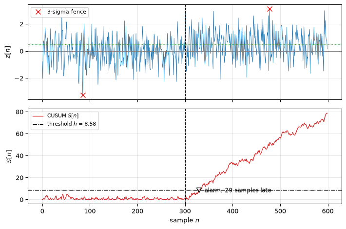
Start with the smallest interesting problem: a stream of independent Gaussian samples whose mean steps from 0 to \(0.5\sigma\) and stays there. Half a standard deviation is a big deal in a measurement system, a 0.5 dB gain error, a slowly leaking seal, a drifting bias, and it is completely invisible one sample at a time.
Show the code
rng = np.random.default_rng(101)n, n_change, delta =600, 300, 0.5z = rng.standard_normal(n)z[n_change:] += deltak, h = design_cusum(delta, 1000.0)alarms, S = cusum_detect(z, k, h, reset=False)first =int(alarms[0])fence = np.abs(z) >3.0before = fence[:n_change].sum()after = fence[n_change:].sum()fig, (ax0, ax1) = plt.subplots(2, 1, figsize=(7.5, 5), sharex=True)ax0.plot(z, color='C0', lw=0.6)ax0.plot(np.where(fence)[0], z[fence], 'rx', ms=7, label='3-sigma fence')ax0.axvline(n_change, color='k', ls='--', lw=1)ax0.axhline(0.0, color='gray', lw=0.8)ax0.axhline(delta, color='C2', lw=0.8, ls=':')ax0.set_ylabel('$z[n]$')ax0.legend(fontsize=8, loc='upper left'); ax0.grid(True, alpha=0.3)ax1.plot(S, color='C3', lw=1.0, label='CUSUM $S[n]$')ax1.axhline(h, color='k', ls='-.', lw=1, label=f'threshold $h$ = {h:.2f}')ax1.axvline(n_change, color='k', ls='--', lw=1)ax1.plot(first, S[first], 'kv', ms=8, mfc='none')ax1.annotate(f'alarm, {first - n_change} samples late', (first +12, S[first] *0.75), fontsize=9)ax1.set_xlabel('sample $n$'); ax1.set_ylabel('$S[n]$')ax1.legend(fontsize=8, loc='upper left'); ax1.grid(True, alpha=0.3)fig.tight_layout(); plt.show()print(f"3-sigma fence: {before} flags in the 300 samples before the change, "f"{after} in the 300 after")print(f"CUSUM (k = {k:.2f}, h = {h:.2f}): alarm at n = {first}, "f"{first - n_change} samples after the change")# The caption's two claims, asserted rather than eyeballed.assert (before, after) == (1, 1), "one flag on each side of the change"assert first - n_change ==29, "the quoted 29-sample delay"
Figure 1: Top: 600 samples of unit-variance noise whose mean steps to 0.5 sigma at n = 300 (dashed line). A three-sigma per-sample fence, the outlier detector of this workshop, flags one sample on each side of the change. Bottom: the CUSUM statistic on the same record, accumulating the log-likelihood ratio for the shift and holding at zero while nothing happens. It crosses its threshold 29 samples after the change, and that threshold was set for one false alarm per 1000 samples, not tuned to this record.
3-sigma fence: 1 flags in the 300 samples before the change, 1 in the 300 after
CUSUM (k = 0.25, h = 8.58): alarm at n = 329, 29 samples after the change
The fence is not badly implemented, and it is not quite blind either. It is slow. Its exceedance rate really does change when the mean shifts, and the size of that change is exactly the problem:
Show the code
p0 =2* norm.sf(3.0) # in controlp1 = norm.sf(3.0- delta) + norm.cdf(-3.0- delta) # after the shiftprint(f"3-sigma exceedance rate: {p0:.5f} before, {p1:.5f} after "f"({p1/p0:.1f}x)")# Samples needed for the two Poisson rates to separate at ~3 standard# errors: a crude but honest order of magnitude.n_needed =9* (p0 + p1) / (p1 - p0)**2print(f"samples needed to call that rate change at ~3 sigma: {n_needed:.0f}")assert n_needed >1000, "the fence needs thousands of samples"
3-sigma exceedance rate: 0.00270 before, 0.00644 after (2.4x)
samples needed to call that rate change at ~3 sigma: 5874
A per-sample detector asks whether this sample is extreme, and no sample here is; recovering the change from the fence means measuring a rate, which takes thousands of samples to do the shift that the CUSUM caught in twenty-nine. The change is only visible in the aggregate, which means the detector has to accumulate, and the moment it accumulates it needs a rule for how long to keep accumulating before deciding it has seen enough.
From Wald’s test to Page’s recursion
Detection theory already gave us the statistic. For standardized data \(z[n] = (y[n]-\mu_0)/\sigma\), the two hypotheses “in control” and “shifted by \(\delta\)” have log-likelihood ratio increment
which is worth reading as a biased accumulator: it adds each observation but pays a toll of \(\delta/2\) per sample. Under \(H_0\) the increment has mean \(-\delta^2/2\), so the sum drifts down; after the change it has mean \(+\delta^2/2\) and drifts up. Those two means are the Kullback-Leibler divergences between the hypotheses in each direction, which is the deepest reason a change of size \(\delta\) costs about \(2h/\delta^2\) samples to detect: information arrives at a fixed rate per sample and you need a fixed amount of it.
Wald’s sequential probability ratio test(Wald 1945) accumulates \(s[n]\) from a known start and stops at whichever of two thresholds it hits first, deciding \(H_1\) above and \(H_0\) below. It is optimal in a precise sense, minimising the expected number of samples among all tests with the same two error probabilities, but it answers the wrong question here: it assumes the change either happened before the test started or not at all.
Page’s insight(Page 1954) was that a change can begin at any time, so the right statistic maximises over every possible starting point:
and that this maximisation, which looks like \(O(n)\) work per sample and unbounded memory, has an exact recursion:
# The entire algorithm. One add, one compare, per sample.def cusum(z, k, h): S, alarms =0.0, []for n, zn inenumerate(z): S =max(0.0, S + zn - k) # accumulate, with a floor at zeroif S >= h: alarms.append(n) S =0.0# restart after acting on the alarmreturn alarms# That recursion IS the maximisation above, not an approximation to it.zz = rng.standard_normal(400)cs = np.cumsum(np.concatenate(([0.0], zz -0.5)))brute = np.array([max(0.0, max(cs[i +1] - cs[i +1- j]for j inrange(1, i +2)))for i inrange(len(zz))])assert np.allclose(brute, cusum_stat(zz, 0.5))print("recursion == max over all n candidate change times, to "f"{np.max(np.abs(brute - cusum_stat(zz, 0.5))):.1e}")
recursion == max over all n candidate change times, to 5.6e-14
The floor at zero is doing all the work. It is what discards a history that has argued against a change, so the statistic never has to be talked back down from a deep negative excursion before it can respond to something real. The reflection at zero is also exactly why the run length has no elementary closed form, which is the subject of the next two sections.
Two facts license the CUSUM as more than a good idea. Lorden (Lorden 1971) proved it asymptotically minimax: among all detectors with a given mean time between false alarms, it minimises the worst-case expected delay over every possible change time and every pre-change history. Moustakides (Moustakides 1986) later proved that optimality exactly, not just asymptotically. This is the same shape of guarantee the Neyman-Pearson lemma gave the matched filter: nothing cleverer exists for this problem.
Two design numbers, and what they cost
A CUSUM has exactly two knobs, and both have plain-language meanings.
The reference value \(k\) is the size of change you care about, halved: \(k = \delta/2\) makes the statistic the exact likelihood ratio for a shift of \(\delta\) standard deviations. Choosing \(k\) is choosing what counts as a change worth reporting rather than as normal wander. It is not a sensitivity dial to be tuned until the alarms look right.
The threshold \(h\) buys the false-alarm rate. Both are quoted in \(\sigma\) units here; a threshold expressed in log-likelihood units is \(\delta h\), and that factor is the easiest way to ship a detector wrong by a constant, which is why changedet.py never applies it silently.
Performance is a pair of average run lengths: \(\mathrm{ARL}_0\), the mean samples to a false alarm when nothing changes, and \(\mathrm{ARL}_1\), the mean delay from the change to the alarm. Raising \(h\) improves one and ruins the other, and the whole design consists of buying the delay you can live with at the false-alarm rate you can afford.
A run-length formula quoted from memory is a Cramer-Rao bound in another costume
As the sinusoid page shows the hard way, a closed-form bound is only as good as the parameterisation it was written for, and the way to find out is to measure it. Run lengths are worse than bounds in this respect, because the literature carries several ARL approximations that differ by which sidedness, which drift convention, and whether an overshoot correction is included, and they all look equally plausible on a slide.
Nothing on this page is quoted on faith. Every run length exists in three independent versions, and the tests require them to agree: Siegmund’s closed form(Siegmund 1985), a diffusion approximation; a Markov-chain quadrature of the underlying integral equation (Brook and Evans 1972); and direct simulation of the recursion itself. Where they disagree, the section below says so and says by how much.
Siegmund’s approximation treats the statistic as Brownian motion between a reflecting barrier at zero and an absorbing one at \(h\):
\[\mathrm{ARL} \approx \frac{e^{-2\Delta b} + 2\Delta b - 1}{2\Delta^2}, \qquad \Delta = \delta - k, \qquad b = h + 1.166\]
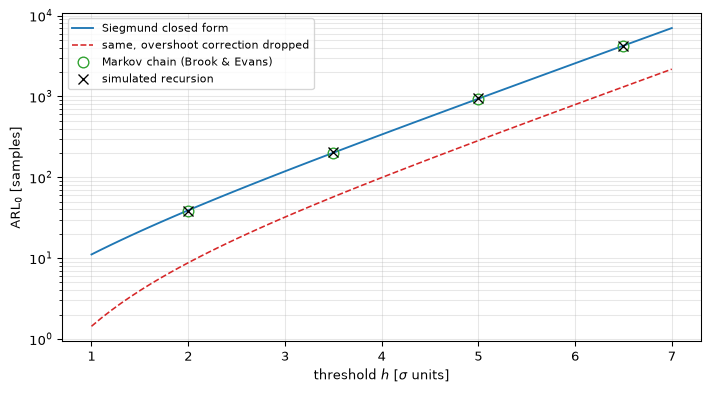
with \(\delta = 0\) giving \(\mathrm{ARL}_0\) and \(\delta = 2k\) giving the delay at the design shift. The constant in \(b\) is an overshoot correction: a discrete-time random walk does not stop politely at the threshold, it jumps past it, and pretending otherwise makes the threshold look harder to reach than it is. That correction is not a refinement, it is the difference between a usable formula and a useless one:
Show the code
k_d =0.5h_grid = np.linspace(1.0, 7.0, 60)siegmund = np.array([arl_siegmund(k_d, hh, 0.0) for hh in h_grid])uncorrected = np.array([(np.exp(2* k_d * hh) -2* k_d * hh -1)/ (2* k_d**2) for hh in h_grid])h_pts = np.array([2.0, 3.5, 5.0, 6.5])markov = np.array([arl_markov(k_d, hh, 0.0) for hh in h_pts])mc_rng = np.random.default_rng(102)mc = np.array([arl_mc(k_d, hh, 0.0, trials=4000, rng=mc_rng)for hh in h_pts])fig, ax = plt.subplots(figsize=(7.5, 4.2))ax.semilogy(h_grid, siegmund, 'C0', lw=1.4, label='Siegmund closed form')ax.semilogy(h_grid, uncorrected, 'C3', lw=1.2, ls='--', label='same, overshoot correction dropped')ax.semilogy(h_pts, markov, 'o', color='C2', ms=8, mfc='none', label='Markov chain (Brook & Evans)')ax.semilogy(h_pts, mc[:, 0], 'kx', ms=8, label='simulated recursion')ax.set_xlabel('threshold $h$ [$\\sigma$ units]')ax.set_ylabel('$\\mathrm{ARL}_0$ [samples]')ax.legend(fontsize=8, loc='upper left'); ax.grid(True, alpha=0.3, which='both')fig.tight_layout(); plt.show()for hh, mk, (m, se) inzip(h_pts, markov, mc):print(f"h = {hh:.1f}: Markov {mk:8.1f}, simulated {m:8.1f} +- {se:5.1f}, "f"Siegmund {arl_siegmund(k_d, hh, 0.0):8.1f}")assertabs(mk - m) <4* se +0.02* mk, "the routes must agree"# The caption's factor-of-three claim at h = 5, pinned.drop = arl_markov(k_d, 5.0, 0.0) / ((np.exp(2* k_d *5.0)-2* k_d *5.0-1) / (2* k_d**2))print(f"dropping the overshoot correction at h = 5 understates ARL0 "f"by {drop:.1f}x")assert2.9< drop <3.4, "the quoted factor of three"
Figure 2: Mean samples to a false alarm against threshold, for a CUSUM designed to catch a one-sigma shift (k = 0.5). The three routes lie on top of each other over four decades: Siegmund’s closed form (line), the Brook-Evans Markov quadrature (circles), and direct simulation of the recursion (crosses, 4000 runs each, error bars smaller than the markers). The dashed line is the same closed form with the overshoot correction dropped; it understates the run length by a factor of 3.3 at h = 5 and gets worse with h, which is what an uncorrected diffusion argument buys you.
h = 2.0: Markov     38.5, simulated     38.4 +-   0.6, Siegmund     39.1
h = 3.5: Markov    199.6, simulated    203.9 +-   3.2, Siegmund    201.2
h = 5.0: Markov    930.9, simulated    963.9 +-  14.7, Siegmund    938.2
h = 6.5: Markov   4219.5, simulated   4234.5 +-  68.1, Siegmund   4251.7
dropping the overshoot correction at h = 5 understates ARL0 by 3.3x
Where the closed form stops being true
Siegmund’s approximation is a diffusion argument: it models a sum of discrete steps as continuous Brownian motion, which is a good story exactly when each step is small compared with the distance to the threshold. That is the regime a CUSUM is built for, because a CUSUM exists to catch changes too small to see in one sample. But the assumption is real, and it is worth knowing where it breaks rather than discovering it in a design review.
Show the code
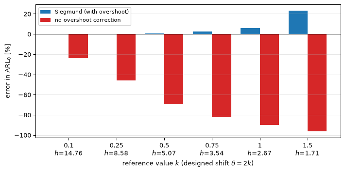
k_sweep = np.array([0.1, 0.25, 0.5, 0.75, 1.0, 1.5])err_s, err_w, h_used = [], [], []for kk in k_sweep: _, hh = design_cusum(2* kk, 1000.0) exact = arl_markov(kk, hh, 0.0) wald = (np.exp(2* kk * hh) -2* kk * hh -1) / (2* kk**2) err_s.append(100* (arl_siegmund(kk, hh, 0.0) / exact -1)) err_w.append(100* (wald / exact -1)) h_used.append(hh)assertabs(exact -1000.0) <1.0, "design must hit its target"x = np.arange(len(k_sweep))fig, ax = plt.subplots(figsize=(7.5, 3.8))ax.bar(x -0.2, err_s, 0.4, color='C0', label='Siegmund (with overshoot)')ax.bar(x +0.2, err_w, 0.4, color='C3', label='no overshoot correction')ax.axhline(0, color='k', lw=0.8)ax.set_xticks(x)ax.set_xticklabels([f'{kk:g}\n$h$={hh:.2f}'for kk, hh inzip(k_sweep, h_used)])ax.set_xlabel('reference value $k$ (designed shift $\\delta = 2k$)')ax.set_ylabel('error in $\\mathrm{ARL}_0$ [%]')ax.legend(fontsize=8); ax.grid(True, alpha=0.3, axis='y')fig.tight_layout(); plt.show()for kk, es, ew inzip(k_sweep, err_s, err_w):print(f"k = {kk:4.2f}: Siegmund {es:+7.2f}%, uncorrected {ew:+7.1f}%")assertabs(err_s[2]) <1.0, "within 1% at k = 0.5"assert20< err_s[5] <30, "about a quarter high at k = 1.5"assert-50< err_w[1] <-42and-92< err_w[4] <-88, "the quoted 46% and 90%"assertall(e <0for e in err_w), "the uncorrected error is always optimistic"
Figure 3: How wrong the closed forms are, as a function of how large a shift the detector is tuned for. At each k the threshold is chosen so the exact (Markov) ARL0 is 1000 samples, and the bars show what each approximation claims instead. Siegmund’s form is within 1% out to k = 0.5 and is still usable at k = 1; by k = 1.5 it overstates the run length by a quarter. The uncorrected version is wrong by 46% at k = 0.25 and by 90% at k = 1, in the dangerous direction: it promises far more time between false alarms than the detector delivers.
k = 0.10: Siegmund   -0.02%, uncorrected   -24.0%
k = 0.25: Siegmund   +0.12%, uncorrected   -45.7%
k = 0.50: Siegmund   +0.78%, uncorrected   -69.4%
k = 0.75: Siegmund   +2.44%, uncorrected   -82.6%
k = 1.00: Siegmund   +5.88%, uncorrected   -90.0%
k = 1.50: Siegmund  +23.17%, uncorrected   -96.4%
The practical rule: design with the Markov route, which costs milliseconds and is exact to within its discretization, and keep the closed form for intuition about how\(\mathrm{ARL}_0\) responds to \(h\) (roughly exponentially, which is why thresholds are so much easier to set than they feel). The workshop’s design_cusum does exactly that.
\(\mathrm{ARL}_0\) is a mean, not a horizon
The single most common misreading of a change detector’s specification is treating “one false alarm per 1000 samples” as “safe for 1000 samples”. The CUSUM’s in-control run length is very nearly geometric: it is close to memoryless, because whenever the statistic returns to zero the detector has genuinely forgotten everything. A geometric run length has a standard deviation equal to its mean and a median of only \(\ln 2 \approx 0.69\) times the mean, and its lower quantiles are brutal.
Show the code
rng_g = np.random.default_rng(103)k_g, h_g, trials =0.5, 4.0, 8000lengths = np.zeros(trials)S_g = np.zeros(trials)alive = np.ones(trials, dtype=bool)n_g =0while alive.any() and n_g <60000: n_g +=1 S_g = np.where(alive, np.maximum(0.0, S_g + rng_g.standard_normal(trials)- k_g), 0.0) lengths = np.where(alive, n_g, lengths) alive &= S_g < h_garl0 = lengths.mean()print(f"ARL0 = {arl0:.0f} samples, standard deviation {lengths.std():.0f} "f"(geometric: equal)")print(f"{'quantile':>10}{'measured':>10}{'geometric':>10}{'ratio':>7}")for q in (0.05, 0.10, 0.25, 0.50, 0.90): emp, geo = np.quantile(lengths, q), run_length_quantile(arl0, q)print(f"{q:10.2f}{emp:10.0f}{geo:10.0f}{emp/geo:7.2f}")assertabs(lengths.std() / arl0 -1) <0.05, "std equals mean"for q in (0.25, 0.50, 0.90): # the bulk is geometricassertabs(np.quantile(lengths, q)/ run_length_quantile(arl0, q) -1) <0.07, f"bulk at q={q}"# The far lower tail is NOT geometric, and errs in the safe direction:# the statistic must climb from zero, so very short runs are rarer than# memorylessness predicts.assert np.quantile(lengths, 0.05) >1.2* run_length_quantile(arl0, 0.05)short = np.mean(lengths <0.1* arl0)print(f"\n{short:.1%} of runs false-alarm within the first 10% of the ARL0")assert0.05< short <0.10
ARL0 = 338 samples, standard deviation 329 (geometric: equal)
  quantile   measured  geometric   ratio
      0.05         24         17    1.38
      0.10         42         36    1.18
      0.25        103         97    1.06
      0.50        237        234    1.01
      0.90        765        778    0.98

7.5% of runs false-alarm within the first 10% of the ARL0
The mean and standard deviation match, and the bulk of the distribution follows the geometric law to within a few percent. So a detector specified at \(\mathrm{ARL}_0 = 1000\) samples has roughly a one-in-eleven chance of crying wolf inside its first 100, and its median time to a false alarm is only about 690 samples, not 1000. If the cost of a false alarm is a technician driving to a site, that distribution, not its mean, is the number to quote. This is the sequential analogue of the ROC page’s third habit: a finite experiment delivers the granularity of its event counts, not the asymptotic promise.
The one place the geometric law breaks is the extreme lower tail, and it breaks in the reassuring direction. A memoryless process can end immediately; this one cannot, because the statistic has to climb from zero to \(h\), which takes several samples however lucky the noise is. Very short runs are therefore rarer than the geometric model predicts (measured above at the 5th percentile), so using it to bound the early-false-alarm risk is conservative rather than optimistic.
The trade curve: delay against false alarms
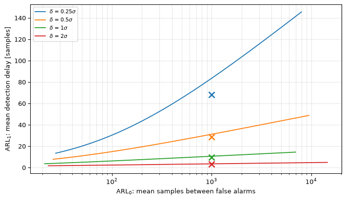
With the run lengths trustworthy, the design space can be drawn. This plot is to change detection what the ROC is to fixed-window detection: the complete menu of trades, with the physics fixed and only the threshold moving.
Show the code
fig, ax = plt.subplots(figsize=(7.5, 4.4))sim_rng = np.random.default_rng(104)for delta_i, colour inzip((0.25, 0.5, 1.0, 2.0), ('C0', 'C1', 'C2', 'C3')): k_i = delta_i /2 hs = np.linspace(0.5, 1.0+6.0/max(delta_i, 0.3), 40) a0 = np.array([arl_markov(k_i, hh, 0.0) for hh in hs]) a1 = np.array([arl_markov(k_i, hh, delta_i) for hh in hs]) keep = (a0 >20) & (a0 <1e5) ax.semilogx(a0[keep], a1[keep], colour, lw=1.4, label=f'$\\delta$ = {delta_i:g}$\\sigma$') _, h_i = design_cusum(delta_i, 1000.0)def det(zz, k_=k_i, h_=h_i): a, _ = cusum_detect(zz, k_, h_, reset=False)returnint(a[0]) iflen(a) elseNone d_mean, d_se = detection_delay_mc(det, delta_i, trials=400, burn_in=150, rng=sim_rng, max_samples=3000) ax.plot(1000, d_mean, 'x', color=colour, ms=9, mew=2) theory = arl_markov(k_i, h_i, delta_i)print(f"delta = {delta_i:4.2f}: h = {h_i:5.3f}, theory delay "f"{theory:7.2f}, warm-started simulation {d_mean:7.2f} "f"+- {d_se:.2f}")assert d_mean < theory +4* d_se, "warm start cannot be slower"assert d_mean >0.55* theory, "nor absurdly faster"ax.set_xlabel('$\\mathrm{ARL}_0$: mean samples between false alarms')ax.set_ylabel('$\\mathrm{ARL}_1$: mean detection delay [samples]')ax.legend(fontsize=8); ax.grid(True, alpha=0.3, which='both')fig.tight_layout(); plt.show()# The caption's "2/delta^2 per log unit" slope claim, measured on the curves.print("\nextra delay per natural log unit of ARL0, and per decade:")for delta_i in (0.25, 0.5, 1.0, 2.0): k_i = delta_i /2 h_a, h_b = design_cusum(delta_i, 300.0)[1], design_cusum(delta_i, 3000.0)[1] per_decade = arl_markov(k_i, h_b, delta_i) - arl_markov(k_i, h_a, delta_i) slope = per_decade / np.log(10.0)print(f" delta = {delta_i:4.2f}: {slope:6.2f} per log unit "f"(2/delta^2 = {2/delta_i**2:6.2f}), {per_decade:6.1f} per decade")assert0.6< slope / (2/ delta_i**2) <1.5
delta = 0.25: h = 13.149, theory delay   83.42, warm-started simulation   68.03 +- 2.59
delta = 0.50: h = 8.585, theory delay   31.08, warm-started simulation   28.72 +- 0.99
delta = 1.00: h = 5.071, theory delay   10.52, warm-started simulation    9.76 +- 0.29
delta = 2.00: h = 2.665, theory delay    3.41, warm-started simulation    3.15 +- 0.08
Figure 4: Detection delay against mean time between false alarms, sweeping the threshold, for CUSUMs matched to four shift sizes. The horizontal axis is logarithmic, and the curves are close to straight on it: buying a decade more time between false alarms costs a roughly constant number of extra samples of delay. That constant is about 2/delta^2 per natural log unit of ARL0, so it is shift size, not threshold, that sets the price. Crosses are warm-started simulations of the actual detector at ARL0 = 1000, which land at or just below the zero-start theory, as they must: a detector that has been running is already part-way up.
extra delay per natural log unit of ARL0, and per decade:
  delta = 0.25:  27.39 per log unit (2/delta^2 =  32.00),   63.1 per decade
  delta = 0.50:   7.58 per log unit (2/delta^2 =   8.00),   17.4 per decade
  delta = 1.00:   1.97 per log unit (2/delta^2 =   2.00),    4.5 per decade
  delta = 2.00:   0.50 per log unit (2/delta^2 =   0.50),    1.1 per decade
The slope is the useful part. Detection delay grows only logarithmically in the false-alarm rate, so a detector can be made a hundred times quieter for a fixed, and often small, number of extra samples of delay. That is a much better bargain than fixed-window detection offers, and it is the reason sequential methods dominate condition monitoring. The cost is set entirely by \(\delta\): a tenfold quieter detector costs about \(4.6/\delta^2\) extra samples of delay, which is one sample at \(2\sigma\) and about seventy at \(0.25\sigma\).
When you cannot name the change: the GLR
The CUSUM’s optimality comes with a bill: you have to declare \(\delta\) in advance. Declare it too large and small changes crawl in; too small and the detector is slower than it needed to be on the change that actually happened. Often nobody knows: a bearing does not announce its fault size.
The standard answer is the same one detection theory used for composite hypotheses: estimate the unknown parameter by maximum likelihood and test with the estimate plugged in. Here two things are unknown, the change time and the change size, so maximise over both. For a candidate change \(j\) samples ago the ML estimate of the shift is just the mean of those \(j\) samples, and substituting it collapses the log-likelihood ratio to something remarkably clean:
a windowed generalised likelihood ratio(Willsky and Jones 1976; Basseville and Nikiforov 1993). It is two-sided for free, since the square does not care which way the mean moved, and it needs no design shift at all. The window \(W\) is the oldest change the detector still searches for, and it bounds both the memory and the arithmetic: \(O(W)\) per sample against the CUSUM’s \(O(1)\), which is the price of not knowing.
Calibrate the statistic you run, not one of its ingredients
The GLR’s threshold invites a trap that also lies in wait for the voice-pitch capstone’s voicing gate, and it is worth naming because the wrong answer is derived correctly.
For a single candidate change time, \((\sum z)^2/(2j)\) is exactly \(\chi^2_1/2\), whatever \(j\). That is not an approximation, and the tests pin it. It is therefore tempting to set the threshold from \(P(G > h) = \chi^2_1(2h)\) and expect one false alarm per \(1/p\) samples.
The detector does not compute that statistic. It computes a maximum over \(W\) correlated candidates, at every sample. Measured below: the naive threshold delivers roughly a quarter of the promised time between false alarms, and the inflation saturates as \(W\) grows, because the candidates are so strongly correlated that widening the search adds only a few effectively independent looks. The correct move is the one the detection-theory embedded page makes on hardware: calibrate by simulating the statistic as deployed.
Show the code
h_naive = glr_threshold_naive(1e-3)print(f"single-candidate threshold for p = 1e-3: h = {h_naive:.3f}")print("measured ARL0 of the deployed maximum-over-W statistic:")trap_rng = np.random.default_rng(105)ratios = {}for W in (1, 10, 50, 200): a, se = glr_arl0_mc(h_naive, W, trials=400, rng=trap_rng) ratios[W] =1000.0/ aprint(f" W = {W:3d}: ARL0 = {a:7.1f} +- {se:5.1f} "f"({ratios[W]:.1f}x more false alarms than promised)")assertabs(ratios[1] -1.0) <0.15, "W = 1 is the honest special case"assert2.5< ratios[50] <5.0, "W = 50 runs several times hot"assertabs(ratios[200] - ratios[50]) <1.5, "the inflation saturates in W"
single-candidate threshold for p = 1e-3: h = 5.414
measured ARL0 of the deployed maximum-over-W statistic:
  W =   1: ARL0 =  1047.6 +-  48.7   (1.0x more false alarms than promised)
  W =  10: ARL0 =   294.9 +-  15.2   (3.4x more false alarms than promised)
  W =  50: ARL0 =   278.2 +-  13.6   (3.6x more false alarms than promised)
  W = 200: ARL0 =   267.4 +-  13.3   (3.7x more false alarms than promised)
\(W = 1\) is the independent special case that proves the closed form itself is right: with one candidate, the naive calculation is exact and the measured run length lands on 1000. Everything above \(W = 1\) is the cost of searching, and it has to be measured because there is no honest formula for it.
Show the code
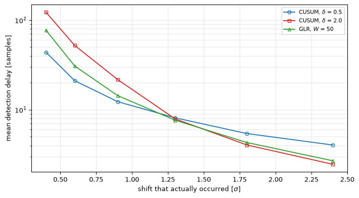
shifts = np.array([0.4, 0.6, 0.9, 1.3, 1.8, 2.4])cmp_rng = np.random.default_rng(106)_, h_c1 = design_cusum(0.5, 1000.0)_, h_c2 = design_cusum(2.0, 1000.0)W_g =50# No formula to inherit: calibrate the GLR threshold by simulating the# statistic as deployed, then verify it on an independent set of runs.h_g_cal = glr_threshold_mc(1000.0, W_g, trials=120, rng=cmp_rng)arl0_g, se_g = glr_arl0_mc(h_g_cal, W_g, trials=400, rng=cmp_rng)print(f"GLR calibrated to h = {h_g_cal:.2f} (W = {W_g}): "f"measured ARL0 = {arl0_g:.0f} +- {se_g:.0f}")assert h_g_cal > glr_threshold_naive(1e-3), "must exceed the naive value"assert600< arl0_g <1700, "the comparison must be near-fairly matched"def make_cusum(k_, h_):def d(zz): a, _ = cusum_detect(zz, k_, h_, reset=False)returnint(a[0]) iflen(a) elseNonereturn ddef glr_det(zz): a, _ = glr_detect(zz, W_g, h_g_cal, reset=False)returnint(a[0]) iflen(a) elseNonecurves = {}for name, det in (('CUSUM, $\\delta$ = 0.5', make_cusum(0.25, h_c1)), ('CUSUM, $\\delta$ = 2.0', make_cusum(1.0, h_c2)), (f'GLR, $W$ = {W_g}', glr_det)): curves[name] = [detection_delay_mc(det, s, trials=250, burn_in=120, rng=cmp_rng, max_samples=1200)[0]for s in shifts]fig, ax = plt.subplots(figsize=(7.5, 4.2))for (name, ys), style inzip(curves.items(), ('C0-o', 'C3-s', 'C2-^')): ax.semilogy(shifts, ys, style, lw=1.4, ms=5, mfc='none', label=name)ax.set_xlabel('shift that actually occurred [$\\sigma$]')ax.set_ylabel('mean detection delay [samples]')ax.legend(fontsize=8); ax.grid(True, alpha=0.3, which='both')fig.tight_layout(); plt.show()small =dict(zip(shifts, curves['CUSUM, $\\delta$ = 0.5']))large =dict(zip(shifts, curves['CUSUM, $\\delta$ = 2.0']))glr =dict(zip(shifts, curves[f'GLR, $W$ = {W_g}']))print(f"at 0.4 sigma: small-shift CUSUM {small[0.4]:.0f}, "f"large-shift CUSUM {large[0.4]:.0f} ({large[0.4]/small[0.4]:.1f}x "f"slower), GLR {glr[0.4]:.0f}")print(f"at 2.4 sigma: small-shift CUSUM {small[2.4]:.1f}, "f"large-shift CUSUM {large[2.4]:.1f} ({small[2.4]/large[2.4]:.1f}x "f"slower the other way), GLR {glr[2.4]:.1f}")# Each CUSUM must win near its own design point, and the GLR must sit# between them at both ends rather than winning or losing outright.assert small[0.4] < large[0.4], "small design wins on a small shift"assert large[2.4] < small[2.4], "large design wins on a large shift"assert small[0.4] < glr[0.4] < large[0.4]assert large[2.4] < glr[2.4] < small[2.4]# The caption claims two ratios, so pin the ratios, not just their operands.assert2.4< large[0.4] / small[0.4] <3.2, "the caption's 2.8x at 0.4 sigma"assert1.4< small[2.4] / large[2.4] <1.9, "the caption's 1.6x at 2.4 sigma"
GLR calibrated to h = 6.77 (W = 50): measured ARL0 = 1004 +- 53
Figure 5: Detection delay against the shift that actually occurred, for three detectors matched to the same measured false-alarm rate (ARL0 near 1000 samples, verified by simulation below). Each CUSUM is fastest near the shift it was designed for and pays elsewhere, and the penalty is asymmetric: guessing too large is the expensive mistake. The delta = 2 design is 2.8x slower than the delta = 0.5 design on a 0.4-sigma drift, while the delta = 0.5 design is only 1.6x slower on a 2.4-sigma jump. The GLR, told nothing about the shift size, is never the fastest and never far off, sitting between the two at both ends. When the change size is genuinely unknown, that flatness is worth more than any single design’s best case.
at 0.4 sigma: small-shift CUSUM 44, large-shift CUSUM 123 (2.8x slower), GLR 77
at 2.4 sigma: small-shift CUSUM 4.0, large-shift CUSUM 2.5 (1.6x slower the other way), GLR 2.7
Back to the noise floor that moved
The CFAR section of the detection page measured something alarming: a one-decibel error in the assumed noise level turns a designed false-alarm rate of \(10^{-3}\) into one in twenty. It then built a detector that re-learns the floor from a sliding reference window, and noted that while the floor is changing the detector simply reports “signal” for as long as its window takes to fill. Whether a persistent rise is an event or a new baseline, it said, is not something a threshold can decide.
It is something a change detector can decide, and the natural place to put one is on the block-energy stream the CFAR is already computing. The statistic is the log of the block energy, because a multiplicative change in noise power is an additive change in log power, which is the form all of this page’s machinery expects.
Show the code
M_blk =64n_blocks, drift_blk =900, 400rng_f = np.random.default_rng(107)def block_log_energy(n_blk, sigma_of_block, rng): e = np.empty(n_blk)for b inrange(n_blk): x = sigma_of_block(b) * rng.standard_normal(M_blk) e[b] = np.log(np.sum(x * x))return esigma_drift =lambda b: 1.0if b < drift_blk else10**(1.0/20) # +1 dB powerlogE = block_log_energy(n_blocks, sigma_drift, rng_f)# Calibrate on the stream the detector sees: mean and spread of the# in-control log-energy, measured, not assumed. For reference, the exact# values for log(chi^2_M) are digamma/trigamma.train = block_log_energy(4000, lambda b: 1.0, np.random.default_rng(108))mu_l, sd_l = train.mean(), train.std()sd_exact = np.sqrt(polygamma(1, M_blk /2))print(f"log-energy spread: measured {sd_l:.4f}, "f"exact sqrt(trigamma(M/2)) {sd_exact:.4f} nats "f"({10* np.log10(np.e) * sd_l:.2f} dB per block)")assertabs(sd_l / sd_exact -1) <0.03, "the chi-square special case"zl = standardize(logE, mu_l, sd_l)shift_1db = np.log(10**(1.0/10)) / sd_l # 1 dB in sigma unitsprint(f"a 1 dB power drift is {shift_1db:.2f} sigma of the log-energy noise")k_f, h_gauss = design_cusum(shift_1db, 1000.0)# ...and check that design against the ACTUAL log-energy stream, which is# log-chi-square, not Gaussian. Measure BOTH arms separately, so the# two-sided halving is not mistaken for a distributional effect.cal_rng = np.random.default_rng(109)runs = {'upper': [], 'lower': [], 'two-sided': []}for _ inrange(300): e = standardize(block_log_energy(6000, lambda b: 1.0, cal_rng), mu_l, sd_l)for name, (sig, two) in {'upper': (e, False), 'lower': (-e, False),'two-sided': (e, True)}.items(): a, _ = cusum_detect(sig, k_f, h_gauss, two_sided=two) runs[name].append(a[0] +1iflen(a) else6000)arl0 = {n: float(np.mean(v)) for n, v in runs.items()}skew = polygamma(2, M_blk /2) / polygamma(1, M_blk /2)**1.5print(f"threshold h = {h_gauss:.2f} designed for ARL0 = 1000 under Gaussian "f"theory;\nmeasured on the real log-energy stream, whose skewness is "f"{skew:+.3f}:")for n in ('upper', 'lower', 'two-sided'):print(f" {n:10s} ARL0 = {arl0[n]:6.0f}")arl0_real = arl0['two-sided']alarms_f, S_f = cusum_detect(zl, k_f, h_gauss, two_sided=True, reset=False)first_f =int(alarms_f[0])fig, (ax0, ax1) = plt.subplots(2, 1, figsize=(7.5, 5), sharex=True)ax0.plot(10* np.log10(np.exp(logE)), color='C0', lw=0.5)ax0.axvline(drift_blk, color='k', ls='--', lw=1)ax0.set_ylabel('block energy [dB]'); ax0.grid(True, alpha=0.3)ax1.plot(S_f, color='C3', lw=1.0, label='two-sided CUSUM')ax1.axhline(h_gauss, color='k', ls='-.', lw=1, label=f'$h$ = {h_gauss:.2f}')ax1.axvline(drift_blk, color='k', ls='--', lw=1)ax1.plot(first_f, S_f[first_f], 'kv', ms=8, mfc='none')ax1.annotate(f'{first_f - drift_blk} blocks late', (first_f +12, S_f[first_f] *0.7), fontsize=9)ax1.set_xlabel('block'); ax1.set_ylabel('$S$')ax1.legend(fontsize=8, loc='upper left'); ax1.grid(True, alpha=0.3)fig.tight_layout(); plt.show()# One realization is one draw; quote the mean delay too.delay_rng = np.random.default_rng(110)delays = []for _ inrange(300): e = block_log_energy(120, lambda b: 1.0if b <40else10**(1.0/20), delay_rng) a, _ = cusum_detect(standardize(e, mu_l, sd_l), k_f, h_gauss, two_sided=True, reset=False) post = [i for i in a if i >=40]if post: delays.append(post[0] -40+1)mean_delay =float(np.mean(delays))print(f"drift flagged {first_f - drift_blk} blocks after it started; "f"mean over 300 runs {mean_delay:.1f} blocks "f"({mean_delay * M_blk:.0f} samples)")assert first_f > drift_blk, "no alarm before the drift"assert first_f - drift_blk ==5, "the quoted single-realization delay"assertabs(mean_delay -6.3) <0.6, "the quoted mean delay"# Left skew (negative) must make the LOWER arm the trigger-happy one, and# the two arms together must be quicker than either alone.assert skew <-0.15, "log chi-square is left-skewed"assert arl0['lower'] < arl0['upper'], "the long tail is the lower one"assert arl0_real <min(arl0['upper'], arl0['lower'])# Competing risks: the two-sided rate is the sum of the two arms' rates.combined =1/ (1/ arl0['upper'] +1/ arl0['lower'])print(f" two arms combined as competing risks: {combined:.0f}")assertabs(combined / arl0_real -1) <0.15assert arl0_real <700, "as shipped it alarms about twice as often as designed"
log-energy spread: measured 0.1777, exact sqrt(trigamma(M/2)) 0.1782 nats (0.77 dB per block)
a 1 dB power drift is 1.30 sigma of the log-energy noise
threshold h = 4.05 designed for ARL0 = 1000 under Gaussian theory;
measured on the real log-energy stream, whose skewness is -0.178:
  upper      ARL0 =   1249
  lower      ARL0 =    799
  two-sided  ARL0 =    516
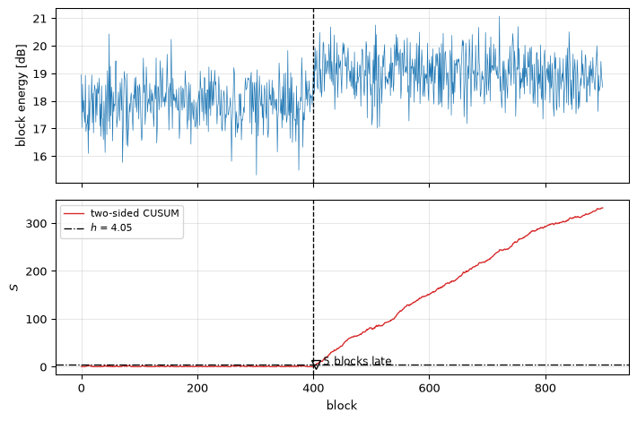
Figure 6: A 1 dB noise-floor drift, the exact error that breaks a fixed threshold, arriving at block 400 of a 64-sample-block energy stream. Top: block energy in dB; the drift is 1 dB against a per-block spread of 0.77 dB, so it is lost in the block-to-block scatter. Bottom: a two-sided CUSUM on the standardized log-energy, which flags this realization 5 blocks after the drift starts (6.3 blocks averaged over 300 runs, printed below). The threshold came from the Gaussian design theory and was then checked against the log-energy stream itself rather than trusted.
drift flagged 5 blocks after it started; mean over 300 runs 6.3 blocks (406 samples)
  two arms combined as competing risks: 487
Two things in that cell are worth more than the picture.
The first is that an exact special case is available, and used. The logarithm of a \(\chi^2_M\) variable has variance \(\psi'(M/2)\) and skewness \(\psi''(M/2)\,\psi'(M/2)^{-3/2}\), the trigamma and tetragamma functions, so the measured spread of the log-energy stream is checked against a closed form that owes nothing to the simulation. It agrees to 0.3%. That is the rule worth borrowing: Monte Carlo and an independent special case, never one alone.
The second is that the design does not survive contact with the stream, and the reason is not the one a quick glance suggests. A threshold computed for Gaussian increments delivers about half its nominal \(\mathrm{ARL}_0\) here, and it would be easy to write that off as “two arms instead of one, so twice the alarms”. The measurement says otherwise: the two arms are not symmetric. Log-energy is left-skewed (skewness \(-0.18\) at \(M = 64\)), so its long tail points downward, and the arm watching for a drop fires distinctly more often than the arm watching for a rise, which is itself quieter than Gaussian theory promised. Adding the two arms’ rates as competing risks reproduces the measured two-sided run length; assuming symmetry does not.
Neither effect is large, and neither is predictable in size from the outside. That is the whole argument for measuring: the Gaussian theory is what tells you which threshold to try, and the log-energy stream is what tells you what that threshold actually costs. Design on the theory, ship on the measurement.
On hardware
This is the cheapest detector in the arc by a wide margin. The CUSUM is one subtract, one add, one max, and one compare per sample, with a single machine word of state and no buffer at all, which means it can ride on a stream that is already being computed for another reason: the block energies of a CFAR detector, the residual of a Kalman filter, the output of a lock-in. The GLR is genuinely more expensive, \(O(W)\) multiply-accumulates per sample, and the interesting engineering question is when that buys enough to be worth it.
The embedded companion puts both on the default platforms and finds the risk somewhere other than the arithmetic. Fixed point turns out to be a non-event here: at Q8 the run length is indistinguishable from float64, because the quantization step is a hundredth of the reference value \(k\). What does need care is the logarithm that turns a power ratio into an additive shift, and the baseline \(\mu_0\) that the detector re-estimates after each alarm, which is the one place where a short window quietly buys extra false alarms.
Going further
The pre-change parameters are usually unknown too. Every statistic here needs \(\mu_0\) and \(\sigma\). In practice they come from a training prefix, and a self-starting CUSUM updates them online while refusing to learn from data after a suspected change, which is subtler than it sounds: a detector that adapts to a drift stops being able to see it. Hawkins and Olwell (Hawkins and Olwell 1998) treat the estimated-parameter case, including how much run-length performance the estimation costs.
Bayesian and Shiryaev-Roberts alternatives. Giving the change time a prior yields the Shiryaev-Roberts procedure, which sums the likelihood ratios over candidate change points instead of maximising over them, and is optimal under a different criterion (stationary average delay rather than worst case). Bayesian online changepoint detection extends this to a full posterior over the time since the last change.
Offline segmentation. When the record is complete and the question is “where were the changes”, the sequential constraint disappears and dynamic programming becomes available: binary segmentation, and exact penalized methods such as PELT, find all changepoints jointly. That is a different algorithm class from anything here, and usually the right one for analysing logged data rather than for watching a live stream.
Changes that are not in the mean. A shift in variance, spectrum, or model coefficients fits the same frame: form the log-likelihood ratio for the change you care about and run the same recursion. The log-energy detector above is the variance case in disguise. Gustafsson (Gustafsson 2000) develops the version where the “parameter” is a whole filter, which connects this page directly to adaptive filtering and recursive estimation: a CUSUM on the innovation sequence of an RLS or Kalman filter is the standard way to tell a model that its world has changed.
Allan variance is the natural companion, and is not covered here yet: change detection asks when a sensor’s baseline moved, Allan variance characterises how it wanders when nothing discrete happens at all.
References
Basseville, Michèle, and Igor V. Nikiforov. 1993. Detection of Abrupt Changes: Theory and Application. Englewood Cliffs, NJ: Prentice Hall.
Brook, D., and D. A. Evans. 1972. “An Approach to the Probability Distribution of CUSUM Run Length.”Biometrika 59 (3): 539–49. https://doi.org/10.1093/biomet/59.3.539.
Hawkins, Douglas M., and David H. Olwell. 1998. Cumulative Sum Charts and Charting for Quality Improvement. New York: Springer. https://doi.org/10.1007/978-1-4612-1686-5.
Lorden, G. 1971. “Procedures for Reacting to a Change in Distribution.”The Annals of Mathematical Statistics 42 (6): 1897–1908. https://doi.org/10.1214/aoms/1177693055.
Moustakides, George V. 1986. “Optimal Stopping Times for Detecting Changes in Distributions.”The Annals of Statistics 14 (4): 1379–87. https://doi.org/10.1214/aos/1176350164.
Willsky, A., and H. Jones. 1976. “A Generalized Likelihood Ratio Approach to the Detection and Estimation of Jumps in Linear Systems.”IEEE Transactions on Automatic Control 21 (1): 108–12. https://doi.org/10.1109/TAC.1976.1101146.
Source Code
---title: "Sequential Change Detection"subtitle: "CUSUM, GLR, and the arithmetic of noticing that something moved"description-meta: "CUSUM and GLR for a change you did not schedule: sequential tests, thresholds, and the arithmetic of noticing that something moved."bibliography: ../../references.bib---Every detector on [the detection-theory page](../detection-theory/index.qmd) was handed a window and asked a question about it: is the target in this block, is anyone speaking in this frame. The window ended, the verdict was delivered, the next window began. That framing quietly assumes the thing you are testing against, the noise floor, the baseline, the in-control state, stays put while you work.It does not. Amplifiers warm up. Photodiodes age. A bearing starts to wear. A microphone gets covered by a sleeve. The question that matters for a system that runs for months is not "is there a signal in this block?" but **"has the process I have been watching stopped being the process it was?"**, and it differs from everything upstream in three ways. There is no window: the data arrives one sample at a time and never ends. There is no false-alarm *probability*: run a detector forever and it alarms eventually, with probability one, so the currency is a false-alarm *rate*. And no single sample is guilty. A change of half a standard deviation is invisible in any one observation and undeniable after fifty.This page builds the two instruments that answer it, both training-free and both cheap enough for a microcontroller: **Page's CUSUM** [@page1954continuous], which is optimal when you can say in advance how large a change matters, and the **windowed GLR**, which estimates the change size as it goes. It also does something the fixed-window pages could take for granted: because there is no closed-form false-alarm probability to quote, the performance numbers here have to be *earned*, three independent ways.::: {.callout-note title="Prerequisites"}Part of the [estimation & detection arc](../estimation-and-detection.qmd); the overview gives the reading order.[Detection theory](../detection-theory/index.qmd) supplies the likelihood ratio and the hypothesis-testing frame this page makes sequential; its [CFAR section](../detection-theory/index.qmd#cfar-when-even-the-noise-level-is-unknown) ends on precisely the question answered here. [Estimation basics](../estimation-basics/index.qmd) supplies the maximum-likelihood machinery the GLR half plugs in, and [outlier detection](../outlier-detection/index.qmd) is the per-sample detector this page is the streaming answer to.:::::: {.callout-tip title="Code"}The implementation is [`changedet.py`](changedet.py). Save [`test_changedet.py`](test_changedet.py) beside it and `pytest test_changedet.py` runs the checks on it.:::```{python}#| echo: falseimport numpy as npimport matplotlib.pyplot as pltfrom scipy.special import polygammafrom scipy.stats import normfrom changedet import (arl_markov, arl_mc, arl_siegmund, cusum_detect, cusum_stat, design_cusum, detection_delay_mc, glr_arl0_mc, glr_detect, glr_threshold_mc, glr_threshold_naive, run_length_quantile, standardize)```<hr>## The change no single sample confesses toStart with the smallest interesting problem: a stream of independent Gaussian samples whose mean steps from 0 to $0.5\sigma$ and stays there. Half a standard deviation is a big deal in a measurement system, a 0.5 dB gain error, a slowly leaking seal, a drifting bias, and it is completely invisible one sample at a time.```{python}#| label: fig-invisible#| fig-cap: "Top: 600 samples of unit-variance noise whose mean steps to 0.5 sigma at n = 300 (dashed line). A three-sigma per-sample fence, the [outlier detector](../outlier-detection/index.qmd) of this workshop, flags one sample on each side of the change. Bottom: the CUSUM statistic on the same record, accumulating the log-likelihood ratio for the shift and holding at zero while nothing happens. It crosses its threshold 29 samples after the change, and that threshold was set for one false alarm per 1000 samples, not tuned to this record."rng = np.random.default_rng(101)n, n_change, delta =600, 300, 0.5z = rng.standard_normal(n)z[n_change:] += deltak, h = design_cusum(delta, 1000.0)alarms, S = cusum_detect(z, k, h, reset=False)first =int(alarms[0])fence = np.abs(z) >3.0before = fence[:n_change].sum()after = fence[n_change:].sum()fig, (ax0, ax1) = plt.subplots(2, 1, figsize=(7.5, 5), sharex=True)ax0.plot(z, color='C0', lw=0.6)ax0.plot(np.where(fence)[0], z[fence], 'rx', ms=7, label='3-sigma fence')ax0.axvline(n_change, color='k', ls='--', lw=1)ax0.axhline(0.0, color='gray', lw=0.8)ax0.axhline(delta, color='C2', lw=0.8, ls=':')ax0.set_ylabel('$z[n]$')ax0.legend(fontsize=8, loc='upper left'); ax0.grid(True, alpha=0.3)ax1.plot(S, color='C3', lw=1.0, label='CUSUM $S[n]$')ax1.axhline(h, color='k', ls='-.', lw=1, label=f'threshold $h$ = {h:.2f}')ax1.axvline(n_change, color='k', ls='--', lw=1)ax1.plot(first, S[first], 'kv', ms=8, mfc='none')ax1.annotate(f'alarm, {first - n_change} samples late', (first +12, S[first] *0.75), fontsize=9)ax1.set_xlabel('sample $n$'); ax1.set_ylabel('$S[n]$')ax1.legend(fontsize=8, loc='upper left'); ax1.grid(True, alpha=0.3)fig.tight_layout(); plt.show()print(f"3-sigma fence: {before} flags in the 300 samples before the change, "f"{after} in the 300 after")print(f"CUSUM (k = {k:.2f}, h = {h:.2f}): alarm at n = {first}, "f"{first - n_change} samples after the change")# The caption's two claims, asserted rather than eyeballed.assert (before, after) == (1, 1), "one flag on each side of the change"assert first - n_change ==29, "the quoted 29-sample delay"```The fence is not badly implemented, and it is not quite blind either. It is *slow*. Its exceedance rate really does change when the mean shifts, and the size of that change is exactly the problem:```{python}#| label: fence-ratep0 =2* norm.sf(3.0) # in controlp1 = norm.sf(3.0- delta) + norm.cdf(-3.0- delta) # after the shiftprint(f"3-sigma exceedance rate: {p0:.5f} before, {p1:.5f} after "f"({p1/p0:.1f}x)")# Samples needed for the two Poisson rates to separate at ~3 standard# errors: a crude but honest order of magnitude.n_needed =9* (p0 + p1) / (p1 - p0)**2print(f"samples needed to call that rate change at ~3 sigma: {n_needed:.0f}")assert n_needed >1000, "the fence needs thousands of samples"```A per-sample detector asks whether *this* sample is extreme, and no sample here is; recovering the change from the fence means measuring a rate, which takes thousands of samples to do the shift that the CUSUM caught in twenty-nine. The change is only visible in the aggregate, which means the detector has to accumulate, and the moment it accumulates it needs a rule for how long to keep accumulating before deciding it has seen enough.<hr>## From Wald's test to Page's recursionDetection theory already gave us the statistic. For standardized data $z[n] = (y[n]-\mu_0)/\sigma$, the two hypotheses "in control" and "shifted by $\delta$" have log-likelihood ratio increment$$s[n] = \ln \frac{f_1(z[n])}{f_0(z[n])} = \delta\left(z[n] - \frac{\delta}{2}\right)$$which is worth reading as a *biased accumulator*: it adds each observation but pays a toll of $\delta/2$ per sample. Under $H_0$ the increment has mean $-\delta^2/2$, so the sum drifts down; after the change it has mean $+\delta^2/2$ and drifts up. Those two means are the Kullback-Leibler divergences between the hypotheses in each direction, which is the deepest reason a change of size $\delta$ costs about $2h/\delta^2$ samples to detect: information arrives at a fixed rate per sample and you need a fixed amount of it.**Wald's sequential probability ratio test** [@wald1945sequential] accumulates $s[n]$ from a known start and stops at whichever of two thresholds it hits first, deciding $H_1$ above and $H_0$ below. It is optimal in a precise sense, minimising the expected number of samples among all tests with the same two error probabilities, but it answers the wrong question here: it assumes the change either happened before the test started or not at all.**Page's insight** [@page1954continuous] was that a change can begin at any time, so the right statistic maximises over every possible starting point:$$S[n] = \max_{1 \le j \le n} \; \sum_{i = n-j+1}^{n} \left(z[i] - k\right), \qquad k = \frac{\delta}{2}$$and that this maximisation, which looks like $O(n)$ work per sample and unbounded memory, has an exact recursion:```{python}#| code-fold: false#| label: cusum-recursion# The entire algorithm. One add, one compare, per sample.def cusum(z, k, h): S, alarms =0.0, []for n, zn inenumerate(z): S =max(0.0, S + zn - k) # accumulate, with a floor at zeroif S >= h: alarms.append(n) S =0.0# restart after acting on the alarmreturn alarms# That recursion IS the maximisation above, not an approximation to it.zz = rng.standard_normal(400)cs = np.cumsum(np.concatenate(([0.0], zz -0.5)))brute = np.array([max(0.0, max(cs[i +1] - cs[i +1- j]for j inrange(1, i +2)))for i inrange(len(zz))])assert np.allclose(brute, cusum_stat(zz, 0.5))print("recursion == max over all n candidate change times, to "f"{np.max(np.abs(brute - cusum_stat(zz, 0.5))):.1e}")```The floor at zero is doing all the work. It is what discards a history that has argued against a change, so the statistic never has to be talked back down from a deep negative excursion before it can respond to something real. The reflection at zero is also exactly why the run length has no elementary closed form, which is the subject of the next two sections.Two facts license the CUSUM as more than a good idea. Lorden [@lorden1971procedures] proved it asymptotically minimax: among all detectors with a given mean time between false alarms, it minimises the worst-case expected delay over every possible change time and every pre-change history. Moustakides [@moustakides1986optimal] later proved that optimality exactly, not just asymptotically. This is the same shape of guarantee the Neyman-Pearson lemma gave the matched filter: nothing cleverer exists for this problem.<hr>## Two design numbers, and what they costA CUSUM has exactly two knobs, and both have plain-language meanings.**The reference value $k$** is the size of change you care about, halved: $k = \delta/2$ makes the statistic the exact likelihood ratio for a shift of $\delta$ standard deviations. Choosing $k$ is choosing what counts as a change worth reporting rather than as normal wander. It is not a sensitivity dial to be tuned until the alarms look right.**The threshold $h$** buys the false-alarm rate. Both are quoted in $\sigma$ units here; a threshold expressed in log-likelihood units is $\delta h$, and that factor is the easiest way to ship a detector wrong by a constant, which is why [`changedet.py`](changedet.py) never applies it silently.Performance is a pair of **average run lengths**: $\mathrm{ARL}_0$, the mean samples to a false alarm when nothing changes, and $\mathrm{ARL}_1$, the mean delay from the change to the alarm. Raising $h$ improves one and ruins the other, and the whole design consists of buying the delay you can live with at the false-alarm rate you can afford.::: {.callout-warning title="A run-length formula quoted from memory is a Cramer-Rao bound in another costume"}As [the sinusoid page](../estimating-a-sinusoid/index.qmd#unknown-frequency-the-1n3-law) shows the hard way, a closed-form bound is only as good as the parameterisation it was written for, and the way to find out is to *measure* it. Run lengths are worse than bounds in this respect, because the literature carries several ARL approximations that differ by which sidedness, which drift convention, and whether an overshoot correction is included, and they all look equally plausible on a slide.Nothing on this page is quoted on faith. Every run length exists in three independent versions, and the tests require them to agree: **Siegmund's closed form** [@siegmund1985sequential], a diffusion approximation; a **Markov-chain quadrature** of the underlying integral equation [@brook1972approach]; and **direct simulation of the recursion itself**. Where they disagree, the section below says so and says by how much.:::Siegmund's approximation treats the statistic as Brownian motion between a reflecting barrier at zero and an absorbing one at $h$:$$\mathrm{ARL} \approx \frac{e^{-2\Delta b} + 2\Delta b - 1}{2\Delta^2}, \qquad \Delta = \delta - k, \qquad b = h + 1.166$$with $\delta = 0$ giving $\mathrm{ARL}_0$ and $\delta = 2k$ giving the delay at the design shift. The constant in $b$ is an **overshoot correction**: a discrete-time random walk does not stop politely at the threshold, it jumps past it, and pretending otherwise makes the threshold look harder to reach than it is. That correction is not a refinement, it is the difference between a usable formula and a useless one:```{python}#| label: fig-arl-routes#| fig-cap: "Mean samples to a false alarm against threshold, for a CUSUM designed to catch a one-sigma shift (k = 0.5). The three routes lie on top of each other over four decades: Siegmund's closed form (line), the Brook-Evans Markov quadrature (circles), and direct simulation of the recursion (crosses, 4000 runs each, error bars smaller than the markers). The dashed line is the same closed form with the overshoot correction dropped; it understates the run length by a factor of 3.3 at h = 5 and gets worse with h, which is what an uncorrected diffusion argument buys you."k_d =0.5h_grid = np.linspace(1.0, 7.0, 60)siegmund = np.array([arl_siegmund(k_d, hh, 0.0) for hh in h_grid])uncorrected = np.array([(np.exp(2* k_d * hh) -2* k_d * hh -1)/ (2* k_d**2) for hh in h_grid])h_pts = np.array([2.0, 3.5, 5.0, 6.5])markov = np.array([arl_markov(k_d, hh, 0.0) for hh in h_pts])mc_rng = np.random.default_rng(102)mc = np.array([arl_mc(k_d, hh, 0.0, trials=4000, rng=mc_rng)for hh in h_pts])fig, ax = plt.subplots(figsize=(7.5, 4.2))ax.semilogy(h_grid, siegmund, 'C0', lw=1.4, label='Siegmund closed form')ax.semilogy(h_grid, uncorrected, 'C3', lw=1.2, ls='--', label='same, overshoot correction dropped')ax.semilogy(h_pts, markov, 'o', color='C2', ms=8, mfc='none', label='Markov chain (Brook & Evans)')ax.semilogy(h_pts, mc[:, 0], 'kx', ms=8, label='simulated recursion')ax.set_xlabel('threshold $h$ [$\\sigma$ units]')ax.set_ylabel('$\\mathrm{ARL}_0$ [samples]')ax.legend(fontsize=8, loc='upper left'); ax.grid(True, alpha=0.3, which='both')fig.tight_layout(); plt.show()for hh, mk, (m, se) inzip(h_pts, markov, mc):print(f"h = {hh:.1f}: Markov {mk:8.1f}, simulated {m:8.1f} +- {se:5.1f}, "f"Siegmund {arl_siegmund(k_d, hh, 0.0):8.1f}")assertabs(mk - m) <4* se +0.02* mk, "the routes must agree"# The caption's factor-of-three claim at h = 5, pinned.drop = arl_markov(k_d, 5.0, 0.0) / ((np.exp(2* k_d *5.0)-2* k_d *5.0-1) / (2* k_d**2))print(f"dropping the overshoot correction at h = 5 understates ARL0 "f"by {drop:.1f}x")assert2.9< drop <3.4, "the quoted factor of three"```<hr>## Where the closed form stops being trueSiegmund's approximation is a *diffusion* argument: it models a sum of discrete steps as continuous Brownian motion, which is a good story exactly when each step is small compared with the distance to the threshold. That is the regime a CUSUM is built for, because a CUSUM exists to catch changes too small to see in one sample. But the assumption is real, and it is worth knowing where it breaks rather than discovering it in a design review.```{python}#| label: fig-siegmund-error#| fig-cap: "How wrong the closed forms are, as a function of how large a shift the detector is tuned for. At each k the threshold is chosen so the exact (Markov) ARL0 is 1000 samples, and the bars show what each approximation claims instead. Siegmund's form is within 1% out to k = 0.5 and is still usable at k = 1; by k = 1.5 it overstates the run length by a quarter. The uncorrected version is wrong by 46% at k = 0.25 and by 90% at k = 1, in the dangerous direction: it promises far more time between false alarms than the detector delivers."k_sweep = np.array([0.1, 0.25, 0.5, 0.75, 1.0, 1.5])err_s, err_w, h_used = [], [], []for kk in k_sweep: _, hh = design_cusum(2* kk, 1000.0) exact = arl_markov(kk, hh, 0.0) wald = (np.exp(2* kk * hh) -2* kk * hh -1) / (2* kk**2) err_s.append(100* (arl_siegmund(kk, hh, 0.0) / exact -1)) err_w.append(100* (wald / exact -1)) h_used.append(hh)assertabs(exact -1000.0) <1.0, "design must hit its target"x = np.arange(len(k_sweep))fig, ax = plt.subplots(figsize=(7.5, 3.8))ax.bar(x -0.2, err_s, 0.4, color='C0', label='Siegmund (with overshoot)')ax.bar(x +0.2, err_w, 0.4, color='C3', label='no overshoot correction')ax.axhline(0, color='k', lw=0.8)ax.set_xticks(x)ax.set_xticklabels([f'{kk:g}\n$h$={hh:.2f}'for kk, hh inzip(k_sweep, h_used)])ax.set_xlabel('reference value $k$ (designed shift $\\delta = 2k$)')ax.set_ylabel('error in $\\mathrm{ARL}_0$ [%]')ax.legend(fontsize=8); ax.grid(True, alpha=0.3, axis='y')fig.tight_layout(); plt.show()for kk, es, ew inzip(k_sweep, err_s, err_w):print(f"k = {kk:4.2f}: Siegmund {es:+7.2f}%, uncorrected {ew:+7.1f}%")assertabs(err_s[2]) <1.0, "within 1% at k = 0.5"assert20< err_s[5] <30, "about a quarter high at k = 1.5"assert-50< err_w[1] <-42and-92< err_w[4] <-88, "the quoted 46% and 90%"assertall(e <0for e in err_w), "the uncorrected error is always optimistic"```The practical rule: design with the Markov route, which costs milliseconds and is exact to within its discretization, and keep the closed form for intuition about *how* $\mathrm{ARL}_0$ responds to $h$ (roughly exponentially, which is why thresholds are so much easier to set than they feel). The workshop's [`design_cusum`](changedet.py) does exactly that.<hr>## $\mathrm{ARL}_0$ is a mean, not a horizonThe single most common misreading of a change detector's specification is treating "one false alarm per 1000 samples" as "safe for 1000 samples". The CUSUM's in-control run length is very nearly **geometric**: it is close to memoryless, because whenever the statistic returns to zero the detector has genuinely forgotten everything. A geometric run length has a standard deviation equal to its mean and a median of only $\ln 2 \approx 0.69$ times the mean, and its lower quantiles are brutal.```{python}#| label: geometric-runlengthrng_g = np.random.default_rng(103)k_g, h_g, trials =0.5, 4.0, 8000lengths = np.zeros(trials)S_g = np.zeros(trials)alive = np.ones(trials, dtype=bool)n_g =0while alive.any() and n_g <60000: n_g +=1 S_g = np.where(alive, np.maximum(0.0, S_g + rng_g.standard_normal(trials)- k_g), 0.0) lengths = np.where(alive, n_g, lengths) alive &= S_g < h_garl0 = lengths.mean()print(f"ARL0 = {arl0:.0f} samples, standard deviation {lengths.std():.0f} "f"(geometric: equal)")print(f"{'quantile':>10}{'measured':>10}{'geometric':>10}{'ratio':>7}")for q in (0.05, 0.10, 0.25, 0.50, 0.90): emp, geo = np.quantile(lengths, q), run_length_quantile(arl0, q)print(f"{q:10.2f}{emp:10.0f}{geo:10.0f}{emp/geo:7.2f}")assertabs(lengths.std() / arl0 -1) <0.05, "std equals mean"for q in (0.25, 0.50, 0.90): # the bulk is geometricassertabs(np.quantile(lengths, q)/ run_length_quantile(arl0, q) -1) <0.07, f"bulk at q={q}"# The far lower tail is NOT geometric, and errs in the safe direction:# the statistic must climb from zero, so very short runs are rarer than# memorylessness predicts.assert np.quantile(lengths, 0.05) >1.2* run_length_quantile(arl0, 0.05)short = np.mean(lengths <0.1* arl0)print(f"\n{short:.1%} of runs false-alarm within the first 10% of the ARL0")assert0.05< short <0.10```The mean and standard deviation match, and the bulk of the distribution follows the geometric law to within a few percent. So a detector specified at $\mathrm{ARL}_0 = 1000$ samples has roughly a one-in-eleven chance of crying wolf inside its first 100, and its *median* time to a false alarm is only about 690 samples, not 1000. If the cost of a false alarm is a technician driving to a site, that distribution, not its mean, is the number to quote. This is the sequential analogue of the [ROC page's third habit](../detection-theory/index.qmd#neyman-pearson-and-the-roc-curve): a finite experiment delivers the granularity of its event counts, not the asymptotic promise.The one place the geometric law breaks is the extreme lower tail, and it breaks in the reassuring direction. A memoryless process can end immediately; this one cannot, because the statistic has to climb from zero to $h$, which takes several samples however lucky the noise is. Very short runs are therefore rarer than the geometric model predicts (measured above at the 5th percentile), so using it to bound the early-false-alarm risk is conservative rather than optimistic.<hr>## The trade curve: delay against false alarmsWith the run lengths trustworthy, the design space can be drawn. This plot is to change detection what the ROC is to fixed-window detection: the complete menu of trades, with the physics fixed and only the threshold moving.```{python}#| label: fig-tradeoff#| fig-cap: "Detection delay against mean time between false alarms, sweeping the threshold, for CUSUMs matched to four shift sizes. The horizontal axis is logarithmic, and the curves are close to straight on it: buying a decade more time between false alarms costs a roughly constant number of extra samples of delay. That constant is about 2/delta^2 per natural log unit of ARL0, so it is shift size, not threshold, that sets the price. Crosses are warm-started simulations of the actual detector at ARL0 = 1000, which land at or just below the zero-start theory, as they must: a detector that has been running is already part-way up."fig, ax = plt.subplots(figsize=(7.5, 4.4))sim_rng = np.random.default_rng(104)for delta_i, colour inzip((0.25, 0.5, 1.0, 2.0), ('C0', 'C1', 'C2', 'C3')): k_i = delta_i /2 hs = np.linspace(0.5, 1.0+6.0/max(delta_i, 0.3), 40) a0 = np.array([arl_markov(k_i, hh, 0.0) for hh in hs]) a1 = np.array([arl_markov(k_i, hh, delta_i) for hh in hs]) keep = (a0 >20) & (a0 <1e5) ax.semilogx(a0[keep], a1[keep], colour, lw=1.4, label=f'$\\delta$ = {delta_i:g}$\\sigma$') _, h_i = design_cusum(delta_i, 1000.0)def det(zz, k_=k_i, h_=h_i): a, _ = cusum_detect(zz, k_, h_, reset=False)returnint(a[0]) iflen(a) elseNone d_mean, d_se = detection_delay_mc(det, delta_i, trials=400, burn_in=150, rng=sim_rng, max_samples=3000) ax.plot(1000, d_mean, 'x', color=colour, ms=9, mew=2) theory = arl_markov(k_i, h_i, delta_i)print(f"delta = {delta_i:4.2f}: h = {h_i:5.3f}, theory delay "f"{theory:7.2f}, warm-started simulation {d_mean:7.2f} "f"+- {d_se:.2f}")assert d_mean < theory +4* d_se, "warm start cannot be slower"assert d_mean >0.55* theory, "nor absurdly faster"ax.set_xlabel('$\\mathrm{ARL}_0$: mean samples between false alarms')ax.set_ylabel('$\\mathrm{ARL}_1$: mean detection delay [samples]')ax.legend(fontsize=8); ax.grid(True, alpha=0.3, which='both')fig.tight_layout(); plt.show()# The caption's "2/delta^2 per log unit" slope claim, measured on the curves.print("\nextra delay per natural log unit of ARL0, and per decade:")for delta_i in (0.25, 0.5, 1.0, 2.0): k_i = delta_i /2 h_a, h_b = design_cusum(delta_i, 300.0)[1], design_cusum(delta_i, 3000.0)[1] per_decade = arl_markov(k_i, h_b, delta_i) - arl_markov(k_i, h_a, delta_i) slope = per_decade / np.log(10.0)print(f" delta = {delta_i:4.2f}: {slope:6.2f} per log unit "f"(2/delta^2 = {2/delta_i**2:6.2f}), {per_decade:6.1f} per decade")assert0.6< slope / (2/ delta_i**2) <1.5```The slope is the useful part. Detection delay grows only *logarithmically* in the false-alarm rate, so a detector can be made a hundred times quieter for a fixed, and often small, number of extra samples of delay. That is a much better bargain than fixed-window detection offers, and it is the reason sequential methods dominate condition monitoring. The cost is set entirely by $\delta$: a tenfold quieter detector costs about $4.6/\delta^2$ extra samples of delay, which is one sample at $2\sigma$ and about seventy at $0.25\sigma$.<hr>## When you cannot name the change: the GLRThe CUSUM's optimality comes with a bill: you have to declare $\delta$ in advance. Declare it too large and small changes crawl in; too small and the detector is slower than it needed to be on the change that actually happened. Often nobody knows: a bearing does not announce its fault size.The standard answer is the same one [detection theory used for composite hypotheses](../detection-theory/index.qmd#going-further): estimate the unknown parameter by maximum likelihood and test with the estimate plugged in. Here two things are unknown, the change time *and* the change size, so maximise over both. For a candidate change $j$ samples ago the ML estimate of the shift is just the mean of those $j$ samples, and substituting it collapses the log-likelihood ratio to something remarkably clean:$$G[n] = \max_{1 \le j \le W} \; \frac{\left(\sum_{i=n-j+1}^{n} z[i]\right)^2}{2j}$$a windowed **generalised likelihood ratio** [@willsky1976generalized; @basseville1993detection]. It is two-sided for free, since the square does not care which way the mean moved, and it needs no design shift at all. The window $W$ is the oldest change the detector still searches for, and it bounds both the memory and the arithmetic: $O(W)$ per sample against the CUSUM's $O(1)$, which is the price of not knowing.::: {.callout-warning title="Calibrate the statistic you run, not one of its ingredients"}The GLR's threshold invites a trap that also lies in wait for [the voice-pitch capstone's voicing gate](../voice-pitch-estimator/index.qmd), and it is worth naming because the wrong answer is *derived correctly*.For a **single** candidate change time, $(\sum z)^2/(2j)$ is exactly $\chi^2_1/2$, whatever $j$. That is not an approximation, and the tests pin it. It is therefore tempting to set the threshold from $P(G > h) = \chi^2_1(2h)$ and expect one false alarm per $1/p$ samples.The detector does not compute that statistic. It computes a **maximum over $W$ correlated candidates, at every sample**. Measured below: the naive threshold delivers roughly a quarter of the promised time between false alarms, and the inflation saturates as $W$ grows, because the candidates are so strongly correlated that widening the search adds only a few effectively independent looks. The correct move is the one the [detection-theory embedded page](../detection-theory/embedded.qmd) makes on hardware: calibrate by simulating the statistic as deployed.:::```{python}#| label: glr-threshold-traph_naive = glr_threshold_naive(1e-3)print(f"single-candidate threshold for p = 1e-3: h = {h_naive:.3f}")print("measured ARL0 of the deployed maximum-over-W statistic:")trap_rng = np.random.default_rng(105)ratios = {}for W in (1, 10, 50, 200): a, se = glr_arl0_mc(h_naive, W, trials=400, rng=trap_rng) ratios[W] =1000.0/ aprint(f" W = {W:3d}: ARL0 = {a:7.1f} +- {se:5.1f} "f"({ratios[W]:.1f}x more false alarms than promised)")assertabs(ratios[1] -1.0) <0.15, "W = 1 is the honest special case"assert2.5< ratios[50] <5.0, "W = 50 runs several times hot"assertabs(ratios[200] - ratios[50]) <1.5, "the inflation saturates in W"```$W = 1$ is the independent special case that proves the closed form itself is right: with one candidate, the naive calculation is exact and the measured run length lands on 1000. Everything above $W = 1$ is the cost of searching, and it has to be measured because there is no honest formula for it.```{python}#| label: fig-cusum-vs-glr#| fig-cap: "Detection delay against the shift that actually occurred, for three detectors matched to the same measured false-alarm rate (ARL0 near 1000 samples, verified by simulation below). Each CUSUM is fastest near the shift it was designed for and pays elsewhere, and the penalty is asymmetric: guessing too large is the expensive mistake. The delta = 2 design is 2.8x slower than the delta = 0.5 design on a 0.4-sigma drift, while the delta = 0.5 design is only 1.6x slower on a 2.4-sigma jump. The GLR, told nothing about the shift size, is never the fastest and never far off, sitting between the two at both ends. When the change size is genuinely unknown, that flatness is worth more than any single design's best case."shifts = np.array([0.4, 0.6, 0.9, 1.3, 1.8, 2.4])cmp_rng = np.random.default_rng(106)_, h_c1 = design_cusum(0.5, 1000.0)_, h_c2 = design_cusum(2.0, 1000.0)W_g =50# No formula to inherit: calibrate the GLR threshold by simulating the# statistic as deployed, then verify it on an independent set of runs.h_g_cal = glr_threshold_mc(1000.0, W_g, trials=120, rng=cmp_rng)arl0_g, se_g = glr_arl0_mc(h_g_cal, W_g, trials=400, rng=cmp_rng)print(f"GLR calibrated to h = {h_g_cal:.2f} (W = {W_g}): "f"measured ARL0 = {arl0_g:.0f} +- {se_g:.0f}")assert h_g_cal > glr_threshold_naive(1e-3), "must exceed the naive value"assert600< arl0_g <1700, "the comparison must be near-fairly matched"def make_cusum(k_, h_):def d(zz): a, _ = cusum_detect(zz, k_, h_, reset=False)returnint(a[0]) iflen(a) elseNonereturn ddef glr_det(zz): a, _ = glr_detect(zz, W_g, h_g_cal, reset=False)returnint(a[0]) iflen(a) elseNonecurves = {}for name, det in (('CUSUM, $\\delta$ = 0.5', make_cusum(0.25, h_c1)), ('CUSUM, $\\delta$ = 2.0', make_cusum(1.0, h_c2)), (f'GLR, $W$ = {W_g}', glr_det)): curves[name] = [detection_delay_mc(det, s, trials=250, burn_in=120, rng=cmp_rng, max_samples=1200)[0]for s in shifts]fig, ax = plt.subplots(figsize=(7.5, 4.2))for (name, ys), style inzip(curves.items(), ('C0-o', 'C3-s', 'C2-^')): ax.semilogy(shifts, ys, style, lw=1.4, ms=5, mfc='none', label=name)ax.set_xlabel('shift that actually occurred [$\\sigma$]')ax.set_ylabel('mean detection delay [samples]')ax.legend(fontsize=8); ax.grid(True, alpha=0.3, which='both')fig.tight_layout(); plt.show()small =dict(zip(shifts, curves['CUSUM, $\\delta$ = 0.5']))large =dict(zip(shifts, curves['CUSUM, $\\delta$ = 2.0']))glr =dict(zip(shifts, curves[f'GLR, $W$ = {W_g}']))print(f"at 0.4 sigma: small-shift CUSUM {small[0.4]:.0f}, "f"large-shift CUSUM {large[0.4]:.0f} ({large[0.4]/small[0.4]:.1f}x "f"slower), GLR {glr[0.4]:.0f}")print(f"at 2.4 sigma: small-shift CUSUM {small[2.4]:.1f}, "f"large-shift CUSUM {large[2.4]:.1f} ({small[2.4]/large[2.4]:.1f}x "f"slower the other way), GLR {glr[2.4]:.1f}")# Each CUSUM must win near its own design point, and the GLR must sit# between them at both ends rather than winning or losing outright.assert small[0.4] < large[0.4], "small design wins on a small shift"assert large[2.4] < small[2.4], "large design wins on a large shift"assert small[0.4] < glr[0.4] < large[0.4]assert large[2.4] < glr[2.4] < small[2.4]# The caption claims two ratios, so pin the ratios, not just their operands.assert2.4< large[0.4] / small[0.4] <3.2, "the caption's 2.8x at 0.4 sigma"assert1.4< small[2.4] / large[2.4] <1.9, "the caption's 1.6x at 2.4 sigma"```<hr>## Back to the noise floor that movedThe [CFAR section](../detection-theory/index.qmd#cfar-when-even-the-noise-level-is-unknown) of the detection page measured something alarming: a **one-decibel** error in the assumed noise level turns a designed false-alarm rate of $10^{-3}$ into one in twenty. It then built a detector that re-learns the floor from a sliding reference window, and noted that while the floor is changing the detector simply reports "signal" for as long as its window takes to fill. Whether a persistent rise is an event or a new baseline, it said, is not something a threshold can decide.It is something a change detector can decide, and the natural place to put one is on the block-energy stream the CFAR is already computing. The statistic is the log of the block energy, because a *multiplicative* change in noise power is an *additive* change in log power, which is the form all of this page's machinery expects.```{python}#| label: fig-floor-drift#| fig-cap: "A 1 dB noise-floor drift, the exact error that breaks a fixed threshold, arriving at block 400 of a 64-sample-block energy stream. Top: block energy in dB; the drift is 1 dB against a per-block spread of 0.77 dB, so it is lost in the block-to-block scatter. Bottom: a two-sided CUSUM on the standardized log-energy, which flags this realization 5 blocks after the drift starts (6.3 blocks averaged over 300 runs, printed below). The threshold came from the Gaussian design theory and was then checked against the log-energy stream itself rather than trusted."M_blk =64n_blocks, drift_blk =900, 400rng_f = np.random.default_rng(107)def block_log_energy(n_blk, sigma_of_block, rng): e = np.empty(n_blk)for b inrange(n_blk): x = sigma_of_block(b) * rng.standard_normal(M_blk) e[b] = np.log(np.sum(x * x))return esigma_drift =lambda b: 1.0if b < drift_blk else10**(1.0/20) # +1 dB powerlogE = block_log_energy(n_blocks, sigma_drift, rng_f)# Calibrate on the stream the detector sees: mean and spread of the# in-control log-energy, measured, not assumed. For reference, the exact# values for log(chi^2_M) are digamma/trigamma.train = block_log_energy(4000, lambda b: 1.0, np.random.default_rng(108))mu_l, sd_l = train.mean(), train.std()sd_exact = np.sqrt(polygamma(1, M_blk /2))print(f"log-energy spread: measured {sd_l:.4f}, "f"exact sqrt(trigamma(M/2)) {sd_exact:.4f} nats "f"({10* np.log10(np.e) * sd_l:.2f} dB per block)")assertabs(sd_l / sd_exact -1) <0.03, "the chi-square special case"zl = standardize(logE, mu_l, sd_l)shift_1db = np.log(10**(1.0/10)) / sd_l # 1 dB in sigma unitsprint(f"a 1 dB power drift is {shift_1db:.2f} sigma of the log-energy noise")k_f, h_gauss = design_cusum(shift_1db, 1000.0)# ...and check that design against the ACTUAL log-energy stream, which is# log-chi-square, not Gaussian. Measure BOTH arms separately, so the# two-sided halving is not mistaken for a distributional effect.cal_rng = np.random.default_rng(109)runs = {'upper': [], 'lower': [], 'two-sided': []}for _ inrange(300): e = standardize(block_log_energy(6000, lambda b: 1.0, cal_rng), mu_l, sd_l)for name, (sig, two) in {'upper': (e, False), 'lower': (-e, False),'two-sided': (e, True)}.items(): a, _ = cusum_detect(sig, k_f, h_gauss, two_sided=two) runs[name].append(a[0] +1iflen(a) else6000)arl0 = {n: float(np.mean(v)) for n, v in runs.items()}skew = polygamma(2, M_blk /2) / polygamma(1, M_blk /2)**1.5print(f"threshold h = {h_gauss:.2f} designed for ARL0 = 1000 under Gaussian "f"theory;\nmeasured on the real log-energy stream, whose skewness is "f"{skew:+.3f}:")for n in ('upper', 'lower', 'two-sided'):print(f" {n:10s} ARL0 = {arl0[n]:6.0f}")arl0_real = arl0['two-sided']alarms_f, S_f = cusum_detect(zl, k_f, h_gauss, two_sided=True, reset=False)first_f =int(alarms_f[0])fig, (ax0, ax1) = plt.subplots(2, 1, figsize=(7.5, 5), sharex=True)ax0.plot(10* np.log10(np.exp(logE)), color='C0', lw=0.5)ax0.axvline(drift_blk, color='k', ls='--', lw=1)ax0.set_ylabel('block energy [dB]'); ax0.grid(True, alpha=0.3)ax1.plot(S_f, color='C3', lw=1.0, label='two-sided CUSUM')ax1.axhline(h_gauss, color='k', ls='-.', lw=1, label=f'$h$ = {h_gauss:.2f}')ax1.axvline(drift_blk, color='k', ls='--', lw=1)ax1.plot(first_f, S_f[first_f], 'kv', ms=8, mfc='none')ax1.annotate(f'{first_f - drift_blk} blocks late', (first_f +12, S_f[first_f] *0.7), fontsize=9)ax1.set_xlabel('block'); ax1.set_ylabel('$S$')ax1.legend(fontsize=8, loc='upper left'); ax1.grid(True, alpha=0.3)fig.tight_layout(); plt.show()# One realization is one draw; quote the mean delay too.delay_rng = np.random.default_rng(110)delays = []for _ inrange(300): e = block_log_energy(120, lambda b: 1.0if b <40else10**(1.0/20), delay_rng) a, _ = cusum_detect(standardize(e, mu_l, sd_l), k_f, h_gauss, two_sided=True, reset=False) post = [i for i in a if i >=40]if post: delays.append(post[0] -40+1)mean_delay =float(np.mean(delays))print(f"drift flagged {first_f - drift_blk} blocks after it started; "f"mean over 300 runs {mean_delay:.1f} blocks "f"({mean_delay * M_blk:.0f} samples)")assert first_f > drift_blk, "no alarm before the drift"assert first_f - drift_blk ==5, "the quoted single-realization delay"assertabs(mean_delay -6.3) <0.6, "the quoted mean delay"# Left skew (negative) must make the LOWER arm the trigger-happy one, and# the two arms together must be quicker than either alone.assert skew <-0.15, "log chi-square is left-skewed"assert arl0['lower'] < arl0['upper'], "the long tail is the lower one"assert arl0_real <min(arl0['upper'], arl0['lower'])# Competing risks: the two-sided rate is the sum of the two arms' rates.combined =1/ (1/ arl0['upper'] +1/ arl0['lower'])print(f" two arms combined as competing risks: {combined:.0f}")assertabs(combined / arl0_real -1) <0.15assert arl0_real <700, "as shipped it alarms about twice as often as designed"```Two things in that cell are worth more than the picture.The first is that an **exact special case** is available, and used. The logarithm of a $\chi^2_M$ variable has variance $\psi'(M/2)$ and skewness $\psi''(M/2)\,\psi'(M/2)^{-3/2}$, the trigamma and tetragamma functions, so the measured spread of the log-energy stream is checked against a closed form that owes nothing to the simulation. It agrees to 0.3%. That is the rule worth borrowing: Monte Carlo *and* an independent special case, never one alone.The second is that the **design does not survive contact with the stream**, and the reason is not the one a quick glance suggests. A threshold computed for Gaussian increments delivers about half its nominal $\mathrm{ARL}_0$ here, and it would be easy to write that off as "two arms instead of one, so twice the alarms". The measurement says otherwise: the two arms are *not* symmetric. Log-energy is left-skewed (skewness $-0.18$ at $M = 64$), so its long tail points downward, and the arm watching for a drop fires distinctly more often than the arm watching for a rise, which is itself quieter than Gaussian theory promised. Adding the two arms' rates as competing risks reproduces the measured two-sided run length; assuming symmetry does not.Neither effect is large, and neither is predictable in size from the outside. That is the whole argument for measuring: the Gaussian theory is what tells you which threshold to *try*, and the log-energy stream is what tells you what that threshold actually costs. Design on the theory, ship on the measurement.<hr>## On hardwareThis is the cheapest detector in the arc by a wide margin. The CUSUM is one subtract, one add, one `max`, and one compare per sample, with a single machine word of state and no buffer at all, which means it can ride on a stream that is already being computed for another reason: the block energies of a CFAR detector, the residual of a Kalman filter, the output of a lock-in. The GLR is genuinely more expensive, $O(W)$ multiply-accumulates per sample, and the interesting engineering question is when that buys enough to be worth it.[The embedded companion](embedded.qmd) puts both on the default platforms and finds the risk somewhere other than the arithmetic. Fixed point turns out to be a non-event here: at Q8 the run length is indistinguishable from float64, because the quantization step is a hundredth of the reference value $k$. What does need care is the logarithm that turns a power ratio into an additive shift, and the baseline $\mu_0$ that the detector re-estimates after each alarm, which is the one place where a short window quietly buys extra false alarms.<hr>## Going further**The pre-change parameters are usually unknown too.** Every statistic here needs $\mu_0$ and $\sigma$. In practice they come from a training prefix, and a self-starting CUSUM updates them online while refusing to learn from data after a suspected change, which is subtler than it sounds: a detector that adapts to a drift stops being able to see it. Hawkins and Olwell [@hawkins1998cumulative] treat the estimated-parameter case, including how much run-length performance the estimation costs.**Bayesian and Shiryaev-Roberts alternatives.** Giving the change time a prior yields the Shiryaev-Roberts procedure, which sums the likelihood ratios over candidate change points instead of maximising over them, and is optimal under a different criterion (stationary average delay rather than worst case). Bayesian online changepoint detection extends this to a full posterior over the time since the last change.**Offline segmentation.** When the record is complete and the question is "where were the changes", the sequential constraint disappears and dynamic programming becomes available: binary segmentation, and exact penalized methods such as PELT, find all changepoints jointly. That is a different algorithm class from anything here, and usually the right one for analysing logged data rather than for watching a live stream.**Changes that are not in the mean.** A shift in variance, spectrum, or model coefficients fits the same frame: form the log-likelihood ratio for the change you care about and run the same recursion. The log-energy detector above is the variance case in disguise. Gustafsson [@gustafsson2000adaptive] develops the version where the "parameter" is a whole filter, which connects this page directly to [adaptive filtering](../adaptive-filtering/index.qmd) and [recursive estimation](../recursive-estimation/index.qmd): a CUSUM on the innovation sequence of an RLS or Kalman filter is the standard way to tell a model that its world has changed.**Allan variance** is the natural companion, and is not covered here yet: change detection asks *when* a sensor's baseline moved, Allan variance characterises *how* it wanders when nothing discrete happens at all.## References::: {#refs}:::