Hypotheses, thresholds, and the ROC: deciding whether a signal is there at all
This workshop is full of detectors that do not call themselves that. The voice-activity gate that stops the pitch tracker from reporting F0 on silence. The energy-and-ZCR thresholds that carve audio into speech and non-speech. The Hampel fences that flag a spike. The lock-in asking whether the LED’s light reaches the photodiode. Every one computes a statistic from the data and compares it to a threshold, every one occasionally cries wolf, every one occasionally sleeps through a burglary, and every one was presented, honestly, as a rule of thumb.
Detection theory is the discipline that replaces the rule of thumb. It answers three questions exactly, for a precisely stated problem: which statistic to compute (the likelihood ratio, and nothing else), where to put the threshold (from the false-alarm rate you can live with), and what performance follows (a curve, not a number: the ROC). This page builds that machinery on the smallest possible problem, then spends it on the three detectors an embedded system actually runs: the matched filter when the waveform is known, the energy detector when it is not, and the CFAR detector when even the noise level is unknown, which is the one the hardware companion puts on live ADC data.
The implementation is detection.py. Save test_detection.py beside it and pytest test_detection.py runs the checks on it.
Two hypotheses, four outcomes
The setup is deliberately spartan. Two competing explanations for the data \(y\):
\[H_0: \text{no signal (noise only)} \qquad H_1: \text{signal present}\]
with the probability density of \(y\) known under each, \(f(y|H_0)\) and \(f(y|H_1)\). A decision rule maps every possible observation to one of the two hypotheses, which is the same as cutting the observation space into two regions. Two hypotheses and two possible decisions give four outcomes, and the two errors have names that radar gave the whole field:
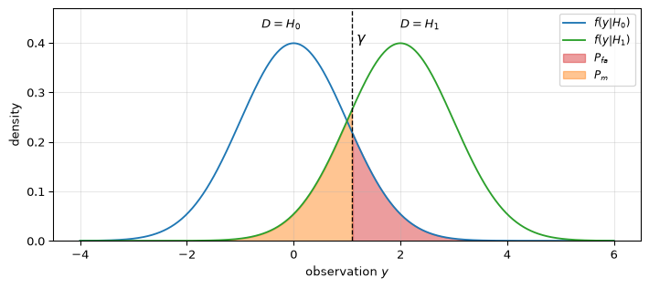
False alarm (type I): deciding \(H_1\) when \(H_0\) is true, with probability \(P_{fa} = P[D = H_1 \mid H_0]\).
Miss (type II): deciding \(H_0\) when \(H_1\) is true, with probability \(P_m = P[D = H_0 \mid H_1]\); its complement is the detection probability\(P_d = 1 - P_m\).
The two errors trade against each other through the threshold, and the whole game is choosing the trade deliberately instead of by folklore. The working example for the next two sections is the smallest detection problem that exists: one sample, \(y = w\) under \(H_0\) versus \(y = A + w\) under \(H_1\), with \(w\) zero-mean Gaussian of variance \(\sigma^2\) and \(A > 0\) known.
Figure 1: The one-sample problem: f(y|H0) and f(y|H1) are unit-variance Gaussians A = 2σ apart, and a threshold γ cuts the axis into the two decision regions. The shaded right tail of the H0 density is the false-alarm probability; the shaded left tail of the H1 density is the miss probability. Sliding γ right shrinks one at the expense of the other; no placement removes either.
One statistic, many thresholds: the likelihood ratio
What is the best decision rule? The remarkable answer, and the organising idea of this page, is that every reasonable notion of “best” produces the same statistic and differs only in where it puts the threshold. Form the likelihood ratio
and the classical decision rules are all of this form:
MAP (minimum probability of error, priors \(P[H_0], P[H_1]\) known): \(\gamma = P[H_0]/P[H_1]\).
Bayes (decision costs \(C_{ij}\) known): \(\gamma = \dfrac{P[H_0](C_{10} - C_{00})}{P[H_1](C_{01} - C_{11})}\), which collapses to MAP for hit/miss costs.
Maximum likelihood (no priors, no costs): \(\gamma = 1\).
Neyman-Pearson (next section): \(\gamma\) set so that \(P_{fa}\) equals a chosen level.
For the one-sample Gaussian problem the log-likelihood ratio is worth working through once, because the simplification pattern repeats for every Gaussian detector on this page:
Monotone in \(y\): comparing \(L(y)\) to any \(\gamma\) is the same as comparing \(y\) itself to a threshold. The optimal detector for a level shift in Gaussian noise is “is the sample big?”, which is reassuring, and the theory’s contribution is not the rule but the calibration of the rule, plus the guarantee that nothing cleverer exists.
From the archive: a 2002 lecture chapter
The primary source for these two sections is a chapter of typeset lecture notes on signal detection (2002, from the author’s reference collection): binary hypothesis testing on a BPAM communication example, MAP and Bayes rules, minimax and Neyman-Pearson, and the correlator detector that reappears below. What the chapter does not cover, the energy detector, ROC machinery beyond a single figure, and CFAR, follows Kay (Kay 1998) and Urkowitz (Urkowitz 1967) instead, with every closed form checked by Monte Carlo on this page and in the tests.
Neyman-Pearson and the ROC curve
Priors and costs are luxuries a measurement system rarely has: what is the prior probability that a pipe is leaking, or the cost ratio of a missed voice frame to a false trigger? The Neyman-Pearson framing needs neither. Fix the false-alarm probability at a level you can tolerate, then maximise the detection probability. The Neyman-Pearson lemma (Neyman and Pearson 1933) says the likelihood-ratio test with \(\gamma\) chosen to hit that \(P_{fa}\) achieves the largest \(P_d\) that any test, of any construction, can reach at that false-alarm rate.
For the one-sample problem everything is closed-form. With the threshold expressed through the target false-alarm rate, the achievable operating points are
\[P_d = Q\!\left(Q^{-1}(P_{fa}) - d\right), \qquad d = \frac{A}{\sigma}\]
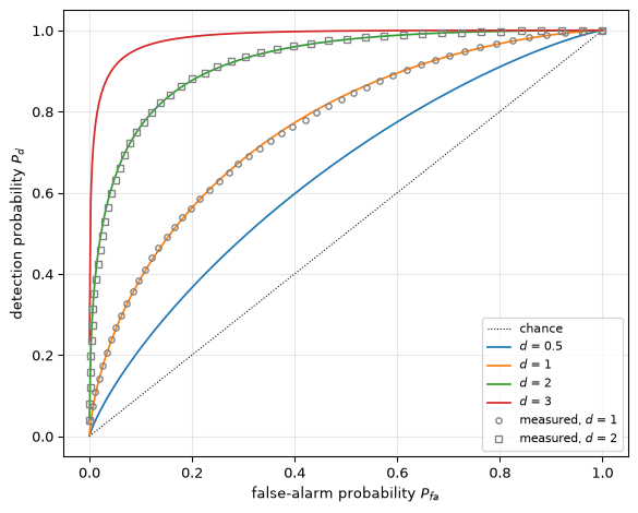
with \(Q\) the Gaussian tail function. Sweeping \(P_{fa}\) from 0 to 1 traces the receiver operating characteristic: the complete menu of trades the detector offers. One number, the deflection\(d\) (how many noise standard deviations the statistic moves when the signal appears), fixes the entire curve.
Show the code
rng = np.random.default_rng(21)pfa_grid = np.linspace(1e-4, 1, 400)fig, ax = plt.subplots(figsize=(6.2, 5))ax.plot([0, 1], [0, 1], 'k:', lw=0.8, label='chance')for d in (0.5, 1.0, 2.0, 3.0): ax.plot(pfa_grid, norm.sf(norm.isf(pfa_grid) - d), lw=1.3, label=f'$d$ = {d:g}')for d, marker in ((1.0, 'o'), (2.0, 's')): fpr, tpr = roc_empirical(rng.standard_normal(20000), rng.standard_normal(20000) + d) ax.plot(fpr[::800], tpr[::800], marker, ms=4, mfc='none', color='gray', label=f'measured, $d$ = {d:g}')# The measured curve must sit on the closed form away from the# sparse extreme-tail region (0.03 covers the binomial wobble of# both axes at 20k trials, slope-amplified; the tests pin the# closed forms tightly with matched thresholds). mid = (fpr >0.02) & (fpr <0.6)assert np.max(np.abs(tpr[mid] - norm.sf(norm.isf(fpr[mid]) - d))) <0.03ax.set_xlabel('false-alarm probability $P_{fa}$')ax.set_ylabel('detection probability $P_d$')ax.legend(fontsize=8, loc='lower right'); ax.grid(True, alpha=0.3)fig.tight_layout(); plt.show()
Figure 2: ROC curves for the Gaussian shift problem at four deflections, with Monte Carlo measurements (20,000 trials per hypothesis) overlaid for d = 1 and d = 2. The chance diagonal is a detector that ignores the data. The curve is the complete performance statement: pick the false-alarm rate you can afford on the horizontal axis and read off the detection rate the physics will sell you.
Three habits of reading a ROC are worth building early. First, comparing detectors at one shared threshold value is meaningless when their statistics live on different scales; comparing whole curves is always fair, which is exactly the lesson the outlier-detection page learned by measurement when its three fence multipliers turned out to be on three different scales. Second, the interesting corner is almost always the far left: real systems run at \(P_{fa}\) of \(10^{-3}\) or below, where the linear plot above compresses everything (plot \(P_d\) against \(\log P_{fa}\) when working there). Third, a ROC from a finite experiment inherits the granularity of its event counts, so the smooth curves here are the asymptotic promise, and the measured points are what a finite record delivers.
The matched filter is the optimal detector
The matched-filtering page derived its correlator by maximising output SNR over all linear filters, using nothing beyond the Cauchy-Schwarz inequality. Detection theory upgrades that result to the strongest statement available. For a known waveform \(s[m]\) in white Gaussian noise,
monotone in the correlation \(\mathbf{y}^T\mathbf{s}\). So the Neyman-Pearson optimal test is the matched filter’s output compared to a threshold, and the optimality is no longer merely against linear filters: by the lemma, no detector of any kind, however nonlinear, achieves a higher \(P_d\) at the same \(P_{fa}\) in this problem. The correlator statistic is Gaussian under both hypotheses with common variance \(\sigma^2 E_s\), so the whole performance question reduces to the one-sample problem with deflection
Only the energy-to-noise ratio enters: waveform shape buys resolution and interference rejection, never detectability, which is the pulse-compression story restated as a theorem.
Which SNR? State the parameterisation, again
The ENR \(E_s/\sigma^2\) is a total-energy ratio: for an \(N\)-sample window it is \(N\) times the per-sample SNR, and for a whole-cycle sinusoid of amplitude \(A\) it is \(N A^2/(2\sigma^2)\), i.e. \(N\) times the \(\eta\) of the sinusoid-estimation page. Detection curves quoted against the wrong axis shift by \(10\log_{10} N\) dB, a far larger error than any approximation on this page. This arc already paid for a parameterisation slip once (the CRLB trap); the same discipline applies to detection statistics, which is why every curve below carries a Monte Carlo check.
The energy detector: the price of not knowing the waveform
Suppose the waveform is unknown: a machine transient, an unpredicted interferer, a voice. With nothing to correlate against, the natural statistic is the energy in the window,
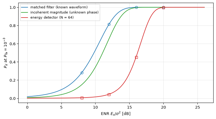
a chi-square with \(N\) degrees of freedom, gaining a noncentrality equal to the ENR when a (deterministic) signal is present (Urkowitz 1967). Both distributions are exact, so threshold and \(P_d\) are again closed-form (energy_detector_threshold, energy_detector_pd), and the comparison with the matched filter at the same \(P_{fa}\) and the same signal energy is the honest cost of ignorance:
Show the code
rng = np.random.default_rng(22)N, pfa_op =64, 1e-3enr_db = np.linspace(0, 26, 200)enr =10**(enr_db /10)fig, ax = plt.subplots(figsize=(7.5, 4.2))ax.plot(enr_db, [matched_filter_pd(pfa_op, e) for e in enr], 'C0', lw=1.4, label='matched filter (known waveform)')ax.plot(enr_db, [incoherent_pd(pfa_op, e) for e in enr], 'C2', lw=1.4, label='incoherent magnitude (unknown phase)')ax.plot(enr_db, [energy_detector_pd(pfa_op, e, N) for e in enr], 'C3', lw=1.4, label=f'energy detector (N = {N})')# Monte Carlo: run each detector for real at a few ENRs.trials =20000s_shape = np.sin(2* np.pi *0.13* np.arange(N) +0.4)s_unit = s_shape / np.sqrt(np.sum(s_shape**2))for e_db in (8.0, 12.0, 16.0, 20.0): e =10**(e_db /10) s = np.sqrt(e) * s_unit # sigma = 1, so ENR = e w = rng.standard_normal((trials, N)) t_mf = (w + s) @ s g_mf = np.sqrt(e) * norm.isf(pfa_op) ax.plot(e_db, np.mean(t_mf > g_mf), 'o', color='C0', mfc='none', ms=6)assertabs(np.mean(t_mf > g_mf) - matched_filter_pd(pfa_op, e)) <0.02 t_ed = np.sum((w + s)**2, axis=1) g_ed = energy_detector_threshold(pfa_op, N) ax.plot(e_db, np.mean(t_ed > g_ed), 's', color='C3', mfc='none', ms=6)assertabs(np.mean(t_ed > g_ed) - energy_detector_pd(pfa_op, e, N)) <0.02ax.set_xlabel('ENR $E_s/\\sigma^2$ [dB]')ax.set_ylabel(f'$P_d$ at $P_{{fa}} = 10^{{-3}}$')ax.legend(fontsize=8, loc='upper left'); ax.grid(True, alpha=0.3)fig.tight_layout(); plt.show()from scipy.optimize import brentqenr_mf = (norm.isf(pfa_op) - norm.isf(0.9))**2enr_ed = brentq(lambda e: energy_detector_pd(pfa_op, e, N) -0.9, 1, 500)gap_db =10* np.log10(enr_ed / enr_mf)print(f"ENR for Pd = 0.9: matched {enr_mf:.1f} ({10*np.log10(enr_mf):.1f} dB), "f"energy {enr_ed:.1f} ({10*np.log10(enr_ed):.1f} dB), gap {gap_db:.2f} dB")assertabs(gap_db -5.3) <0.1, "the quoted 5.3 dB gap at N = 64"
Figure 3: Detection probability against ENR at Pfa = 10⁻³ for a 64-sample window: the matched filter (known waveform), the energy detector (unknown waveform), and the incoherent magnitude detector of the lock-in section below (known frequency, unknown phase). Markers are Monte Carlo measurements (20,000 trials per point) of each actual detector; they sit on their closed forms. At Pd = 0.9 the energy detector needs 5.3 dB more signal energy than the matched filter; the incoherent detector gives up only about 1 dB.
ENR for Pd = 0.9: matched 19.1 (12.8 dB), energy 65.4 (18.2 dB), gap 5.34 dB
The gap is not a constant: it grows with the window. The matched filter’s deflection is \(\sqrt{\text{ENR}}\) regardless of \(N\); the energy statistic’s mean shifts by \(E_s\) while its \(H_0\) standard deviation grows as \(\sigma^2\sqrt{2N}\), giving deflection \(\text{ENR}/\sqrt{2N}\). Equating the two: at low SNR the energy detector needs roughly \(\sqrt{2N}\) times more signal energy, about 3 dB more for every quadrupling of the window (measured at \(P_d = 0.9\): a 3.2 dB gap at \(N = 16\), 5.3 dB at 64, 7.8 dB at 256, 10.5 dB at 1024). Long windows are where knowing the waveform pays most, which is why LIGO correlates against 250,000 templates rather than integrating energy, and why a wakeword detector beats a level meter. When the noise is colored rather than white, both detectors prewhiten first; the theory here then applies verbatim to the whitened data.
CFAR: when even the noise level is unknown
Every threshold above contains \(\sigma^2\). On real hardware that is the quantity you do not have: the noise floor moves with temperature, gain settings, ambient interference, the machine next door. And the chi-square threshold is brutally sensitive to getting it wrong, because at useful window lengths the whole game is played out on the distribution’s thin upper tail:
Show the code
# A 64-sample energy detector designed for Pfa = 1e-3 at an assumed# noise level, fed noise at a slightly different level.g = chi2.isf(1e-3, 64)print("designed Pfa = 1e-3 at N = 64; actual Pfa when the noise is off by:")for db in (0.5, 1.0, 2.0, 3.0): actual = chi2.sf(g /10**(db /10), 64)print(f" +{db:.1f} dB: Pfa = {actual:.3g} ({actual/1e-3:.0f}x the design)")under = chi2.sf(g /10**(-1.0/10), 64)print(f" -1.0 dB: Pfa = {under:.2g} (and Pd falls with it)")assert chi2.sf(g /10**0.1, 64) >0.05, "+1 dB must blow Pfa past 5%"assert under <1e-5, "-1 dB must collapse Pfa (and detections with it)"
designed Pfa = 1e-3 at N = 64; actual Pfa when the noise is off by:
  +0.5 dB: Pfa = 0.0098  (10x the design)
  +1.0 dB: Pfa = 0.0539  (54x the design)
  +2.0 dB: Pfa = 0.405  (405x the design)
  +3.0 dB: Pfa = 0.848  (848x the design)
  -1.0 dB: Pfa = 1.3e-06  (and Pd falls with it)
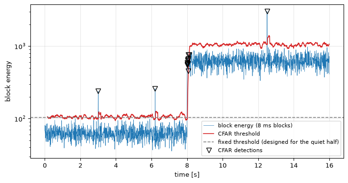
A one-decibel error in the assumed noise level turns a one-in-a-thousand false-alarm rate into one-in-twenty, and a 3 dB error into a detector that fires 85% of the time on pure noise. Underestimating in the other direction silently destroys \(P_d\) instead. No fixed threshold survives contact with a real noise floor; the threshold must be derived from the data.
The cell-averaging CFAR (constant false-alarm rate) detector does exactly that: estimate the noise level from \(N_{\text{ref}}\) reference blocks adjacent to the block under test, and set the threshold as a multiple of that estimate,
The reason this works exactly, not approximately, is that under \(H_0\) both sides are \(\sigma^2\) times chi-square variables, so their ratio is F-distributed with \((M, N_{\text{ref}}M)\) degrees of freedom for \(M\)-sample blocks, and \(\sigma^2\) cancels: the false-alarm rate depends only on \(\alpha\), at every noise level, which is the constant-false-alarm-rate property that names the method. The factor is \(\alpha = F^{-1}(P_{fa}; M, N_{\text{ref}}M)\) (cfar_factor), and for the square-law cells of classical radar (\(M = 2\)) it reduces to the textbook result \(P_{fa} = (1 + \alpha/N_{\text{ref}})^{-N_{\text{ref}}}\), which the tests verify to ten decimal places.
Show the code
rng = np.random.default_rng(23)fs, M, n_ref, n_guard =8000, 64, 16, 2pfa_d =1e-3dur =16.0n =int(dur * fs)t = np.arange(n) / fssigma_t = np.where(t <8.0, 1.0, 10**0.5) # +10 dB power stepx = sigma_t * rng.standard_normal(n)burst = np.sin(2* np.pi *1100* np.arange(M) / fs)amp =2.6burst_blocks =set()enr_bursts = []# The third burst's amplitude scales by sqrt(10) because the noise# VARIANCE stepped by 10: equal ENR means amplitude tracks sigma, not# sigma^2. Getting that wrong costs 5 dB and looks entirely plausible.for t0, scale, s2 in ((3.0, 1.0, 1.0), (6.2, 1.0, 1.0), (12.5, 10**0.5, 10.0)): blk =round(t0 * fs / M) # snap to a block boundary x[blk * M:(blk +1) * M] += amp * scale * burst burst_blocks.add(blk) e_b = np.sum((burst - burst.mean())**2) # mean-removed, as detected enr_bursts.append((amp * scale)**2* e_b / s2)# The caption's equal-ENR claim, pinned: identical to well under 0.1 dB.assert np.ptp(10* np.log10(enr_bursts)) <0.01assertabs(10* np.log10(enr_bursts[0]) -23.3) <0.05e = block_energies(x, M, remove_mean=True)alpha = cfar_factor(pfa_d, M -1, n_ref)det, thr = ca_cfar(e, alpha, n_ref, n_guard)g_fixed = energy_detector_threshold(pfa_d, M -1, 1.0)t_blk = (np.arange(len(e)) +0.5) * M / fsfig, ax = plt.subplots(figsize=(7.5, 4))ax.semilogy(t_blk, e, 'C0', lw=0.5, label='block energy (8 ms blocks)')ax.semilogy(t_blk, thr, 'C3', lw=1.2, label='CFAR threshold')ax.axhline(g_fixed, color='gray', ls='--', lw=1.2, label='fixed threshold (designed for the quiet half)')ax.plot(t_blk[det], e[det], 'kv', ms=7, mfc='none', label='CFAR detections')ax.set_xlabel('time [s]'); ax.set_ylabel('block energy')ax.legend(fontsize=8, loc='lower right'); ax.grid(True, alpha=0.3)fig.tight_layout(); plt.show()step_blk =int(8.0* fs) // Mrelearn =set(range(step_blk, step_blk + n_ref + n_guard +1))extra = [i for i in np.where(det)[0] if i notin burst_blocks]loud = e[step_blk + n_ref + n_guard:]print(f"CFAR detections: bursts {sorted(burst_blocks)} all caught; "f"{len(extra)} step-transient hits, all inside blocks "f"{step_blk}..{step_blk + n_ref + n_guard}: "f"{set(extra) <= relearn}")print(f"fixed threshold in the loud half: fires on "f"{np.mean(loud > g_fixed):.0%} of blocks")assert burst_blocks <=set(np.where(det)[0]), "CFAR must catch all 3 bursts"assertset(extra) <= relearn, "all other hits confined to the step transient"assert np.mean(loud > g_fixed) >0.95, "the fixed threshold must drown"
Figure 4: A CFAR energy detector surviving what breaks a fixed threshold. The record is white noise whose floor steps up 10 dB at t = 8 s, with three one-block tone bursts hidden at 3, 6.2, and 12.5 s, the third scaled with the floor so that all three sit at the same per-block ENR of 23.3 dB (asserted below, not eyeballed). The fixed threshold (gray), set for Pfa = 10⁻³ at the initial noise level, is correct for eight seconds and then fires on every block, permanently. The CFAR threshold (red) rides 16 reference blocks behind the data: it flags the three bursts, fires on the step itself for about a tenth of a second while the loud blocks fill its reference window, and is then correctly calibrated at the new floor. Over this record’s two thousand blocks the design itself promises about two false alarms; this particular noise draw happens to contain none.
CFAR detections: bursts [375, 775, 1562] all caught; 10 step-transient hits, all inside blocks 1000..1018: True
fixed threshold in the loud half: fires on 100% of blocks
The step transient in the figure is worth a pause rather than an apology. For about \(N_{\text{ref}} + N_{\text{guard}}\) blocks after the floor jumps, the detector reports “signal”, because a sustained rise genuinely is indistinguishable from a signal until enough history accumulates to call it the new normal. Whether a persistent change should count as an event or as a new baseline is not something a threshold can decide; it is the defining question of sequential change detection, the arc’s next page, and the CFAR’s re-learning window is the crude first answer. That page also makes the point that this detector’s greatest virtue is a blind spot: a detector engineered to be indifferent to the noise level cannot report that the noise level is drifting, which for a device left in a machine room for three years is often the measurement that mattered.
Beyond that transient, the self-calibration is not free, on two counts, and both are design parameters rather than surprises:
CFAR loss. The reference average is a noisy estimate of the noise level, so \(\alpha\) must be set slightly higher than the known-\(\sigma\) threshold to hold the same \(P_{fa}\), which costs detection. The loss is exactly computable (the signal-present ratio is noncentral-F, cfar_pd) and shrinks fast with the reference window: at \(M = 64\), \(P_{fa} = 10^{-3}\), \(P_d = 0.9\), the extra ENR required is 1.5 dB with 2 reference blocks, 0.4 dB with 8, 0.2 dB with 16, and 0.06 dB with 64. Sixteen blocks of noise history buy performance within a quarter-decibel of clairvoyance.
Show the code
# The quoted loss ladder, computed from the noncentral-F closed form.from scipy.optimize import brentqM_dof, pfa_l =64, 1e-3ideal = brentq(lambda e: energy_detector_pd(pfa_l, e, M_dof) -0.9, 1, 500)print(f"known-sigma energy detector: ENR {ideal:.1f} for Pd = 0.9")losses = {}for nr in (2, 4, 8, 16, 32, 64): need = brentq(lambda e: cfar_pd(pfa_l, e, M_dof, nr) -0.9, 1, 2000) losses[nr] =10* np.log10(need / ideal)print(f" n_ref = {nr:2d}: ENR {need:5.1f}, CFAR loss {losses[nr]:.2f} dB")assert1.4< losses[2] <1.6and0.15< losses[16] <0.30assert losses[64] <0.1assertall(losses[a] > losses[b] for a, b inzip((2, 4, 8, 16, 32), (4, 8, 16, 32, 64)))
known-sigma energy detector: ENR 65.4 for Pd = 0.9
  n_ref =  2: ENR  92.6, CFAR loss 1.51 dB
  n_ref =  4: ENR  78.8, CFAR loss 0.81 dB
  n_ref =  8: ENR  72.1, CFAR loss 0.42 dB
  n_ref = 16: ENR  68.7, CFAR loss 0.22 dB
  n_ref = 32: ENR  67.0, CFAR loss 0.11 dB
  n_ref = 64: ENR  66.2, CFAR loss 0.06 dB
Self-masking. The reference window must contain noise. A signal that leaks into it inflates the estimate and raises the threshold against itself, which is why the implementation keeps guard blocks between the cell under test and the reference window, and why a long-lasting signal (or a second target) can still mask a weaker one. The robust fix is to replace the reference mean with an order statistic such as the median, trading a little extra loss for immunity to contaminated reference cells (Rohling 1983). If that sounds familiar, it should: it is precisely the reasoning that led the outlier-detection page from standard-deviation fences to MAD fences.
The lock-in as a detector, finished
The lock-in page ended on a promise: its no-signal magnitude reading is Rayleigh-distributed, never zero, and deciding “tone present” means thresholding between that Rayleigh floor and the signal’s Rician distribution. The machinery of this page closes that loop in three lines. The two demodulated quadratures are independent Gaussians with per-quadrature variance \(\sigma_z^2\), so \(|z|^2/\sigma_z^2\) is \(\chi^2_2\) under \(H_0\) and noncentral \(\chi'^2_2(\lambda)\) with \(\lambda = A^2/\sigma_z^2\) under \(H_1\): the energy detector’s mathematics with \(N = 2\), applied after the lock-in has already collapsed the record onto one known frequency. The threshold relation is the cleanest closed form in all of detection theory,
and \(P_d\) follows from the noncentral tail (incoherent_pd; equivalently the Marcum Q function of radar).
Show the code
# The closed forms against a simulated quadrature pair, and the price# of not knowing the phase.rng = np.random.default_rng(24)sz, pfa_i =1.0, 1e-3gam = sz * np.sqrt(-2* np.log(pfa_i))trials =200000z0 = sz * (rng.standard_normal(trials) +1j* rng.standard_normal(trials))A_test =4.0z1 = z0 + A_test * np.exp(1j* rng.uniform(0, 2* np.pi, trials))pd_meas = np.mean(np.abs(z1) > gam)pd_closed = incoherent_pd(pfa_i, A_test**2/ sz**2)print(f"threshold {gam:.3f} sigma_z: measured Pfa {np.mean(np.abs(z0) > gam):.2e}, "f"target {pfa_i:.0e}")print(f"Pd at A = 4 sigma_z (random phase): measured {pd_meas:.3f}, "f"closed form {pd_closed:.3f}")from scipy.optimize import brentqlam_coh = (norm.isf(pfa_i) - norm.isf(0.9))**2lam_inc = brentq(lambda l: incoherent_pd(pfa_i, l) -0.9, 1, 200)print(f"lambda for Pd = 0.9: phase known {lam_coh:.1f}, "f"phase unknown {lam_inc:.1f}: incoherent loss "f"{10*np.log10(lam_inc/lam_coh):.2f} dB")assertabs(np.mean(np.abs(z0) > gam) - pfa_i) <3e-4assertabs(pd_meas - pd_closed) <0.01assert0.8<10* np.log10(lam_inc / lam_coh) <1.1
threshold 3.717 sigma_z: measured Pfa 9.30e-04, target 1e-03
Pd at A = 4 sigma_z (random phase): measured 0.660, closed form 0.661
lambda for Pd = 0.9: phase known 19.1, phase unknown 23.8: incoherent loss 0.96 dB
Note what the detector shrugged off: the signal’s phase was random in the simulation, and the magnitude test never noticed. That robustness costs about 1 dB against a hypothetical detector that knew the phase and could test the in-phase channel coherently, a fixed, modest price (the “incoherent loss”) that every envelope detector, from AM radio to this photometer, pays. For the lock-in photometer of the embedded companion, whose noise floor \(\sigma_z\) is predicted by \(\sqrt{S(f_0)/T}\) and verified on hardware, these two formulas turn “is the light path blocked?” into a design equation: choose the false-alarm rate, read off the threshold, and know the detection probability before building anything.
The workshop’s detectors, re-read
With the theory in hand, the rules of thumb scattered across this site resolve into instances of it:
The incoherent detector, now with exact \(P_{fa}\) and \(P_d\)
The re-reading is not a demotion of those pages; the rules work, which is why they shipped. What the theory adds is calibration (a threshold traceable to a false-alarm rate instead of to a demo signal), the guarantee of what cannot be improved (nothing beats the likelihood ratio), and honest limits: all the closed forms on this page assume white Gaussian noise, and real interference is bursty, colored, and non-stationary. The theory then still tells you what to measure, the empirical ROC of the outlier-detection page, even where it can no longer hand you the curve in closed form.
On hardware
Everything in the CFAR section runs comfortably on a microcontroller: block energies are a multiply-accumulate, the reference average is a running sum, and the threshold is one multiply, with no calibration constant anywhere because the CFAR ratio cancels the ADC’s gain, the amplifier’s gain, and the noise level all at once. The embedded companion builds the burst detector of the streaming figure on both default platforms, timer-paced ADC and all, and confirms the designed false-alarm rate on live hardware data.
Going further
Sequential detection. Everything here decides on a fixed-length window. Letting the test keep observing until it is sure (Wald’s sequential probability ratio test) or watching for a change in distribution (CUSUM, GLR) is strictly more powerful for monitoring problems. That is now its own page, which picks up the CFAR’s re-learning transient and the composite-hypothesis thread below and runs both to their sequential conclusions; Allan variance remains this arc’s other deferred item.
Composite hypotheses. This page’s \(H_1\) always had known parameters (or none). When amplitude, frequency, or arrival time are unknown, the generalised likelihood ratio test estimates them first (usually by maximum likelihood, tying back to estimation basics) and detects with the estimate plugged in; the matched-filter bank of LIGO is exactly a GLRT over a gridded parameter space.
Random signals. For a Gaussian random signal in Gaussian noise the optimal statistic becomes a quadratic form (the estimator-correlator), interpolating between the matched filter and the energy detector; Kay’s Volume II (Kay 1998) covers the whole ladder.
M-ary decisions. Choosing among more than two hypotheses (which symbol, which keyword) generalises everything here to a bank of correlators and a maximum; the archive chapter closes with it, and the MFCC wakeword detector is a working example wearing feature-space clothes.
References
Kay, Steven M. 1998. Fundamentals of Statistical Signal Processing, Volume II: Detection Theory. Upper Saddle River, NJ: Prentice Hall PTR.
Neyman, Jerzy, and Egon S. Pearson. 1933. “On the Problem of the Most Efficient Tests of Statistical Hypotheses.”Philosophical Transactions of the Royal Society of London. Series A 231: 289–337. https://doi.org/10.1098/rsta.1933.0009.
Rohling, Hermann. 1983. “Radar CFAR Thresholding in Clutter and Multiple Target Situations.”IEEE Transactions on Aerospace and Electronic Systems AES-19 (4): 608–21. https://doi.org/10.1109/TAES.1983.309350.
Urkowitz, Harry. 1967. “Energy Detection of Unknown Deterministic Signals.”Proceedings of the IEEE 55 (4): 523–31. https://doi.org/10.1109/PROC.1967.5573.
Source Code
---title: "Detection Theory"subtitle: "Hypotheses, thresholds, and the ROC: deciding whether a signal is there at all"description-meta: "Deciding whether a signal is there at all: hypothesis testing, the likelihood ratio, thresholds, and how to read an ROC curve."bibliography: ../../references.bib---This workshop is full of detectors that do not call themselves that. The [voice-activity gate](../pitch-detection/index.qmd#voice-activity-detection) that stops the pitch tracker from reporting F0 on silence. The [energy-and-ZCR thresholds](../statistical-features/index.qmd#a-two-feature-decision-rule) that carve audio into speech and non-speech. The [Hampel fences](../outlier-detection/index.qmd) that flag a spike. The [lock-in](../lock-in-detection/index.qmd#the-lock-in-as-a-detector) asking whether the LED's light reaches the photodiode. Every one computes a statistic from the data and compares it to a threshold, every one occasionally cries wolf, every one occasionally sleeps through a burglary, and every one was presented, honestly, as a rule of thumb.Detection theory is the discipline that replaces the rule of thumb. It answers three questions exactly, for a precisely stated problem: which statistic to compute (the likelihood ratio, and nothing else), where to put the threshold (from the false-alarm rate you can live with), and what performance follows (a curve, not a number: the ROC). This page builds that machinery on the smallest possible problem, then spends it on the three detectors an embedded system actually runs: the matched filter when the waveform is known, the energy detector when it is not, and the CFAR detector when even the noise level is unknown, which is the one [the hardware companion](embedded.qmd) puts on live ADC data.::: {.callout-note title="Prerequisites"}Part of the [estimation & detection arc](../estimation-and-detection.qmd); the overview gives the reading order.[Estimation basics](../estimation-basics/index.qmd) supplies the likelihood-function machinery this page reuses for decisions. The [ROC section of outlier detection](../outlier-detection/index.qmd#which-detector-at-which-threshold-the-roc-curve) is the measured warm-up act for the theory here, and [noise and SNR](../../basics/03-noise-snr.qmd) covers the Gaussian background.:::::: {.callout-tip title="Code"}The implementation is [`detection.py`](detection.py). Save [`test_detection.py`](test_detection.py) beside it and `pytest test_detection.py` runs the checks on it.:::```{python}#| echo: falseimport numpy as npimport matplotlib.pyplot as pltfrom scipy.stats import norm, chi2, ncx2from detection import (matched_filter_pd, energy_detector_pd, energy_detector_threshold, incoherent_pd, cfar_factor, cfar_pd, roc_empirical, block_energies, ca_cfar)```<hr>## Two hypotheses, four outcomesThe setup is deliberately spartan. Two competing explanations for the data $y$:$$H_0: \text{no signal (noise only)} \qquad H_1: \text{signal present}$$with the probability density of $y$ known under each, $f(y|H_0)$ and $f(y|H_1)$. A **decision rule** maps every possible observation to one of the two hypotheses, which is the same as cutting the observation space into two regions. Two hypotheses and two possible decisions give four outcomes, and the two errors have names that radar gave the whole field:- **False alarm** (type I): deciding $H_1$ when $H_0$ is true, with probability $P_{fa} = P[D = H_1 \mid H_0]$.- **Miss** (type II): deciding $H_0$ when $H_1$ is true, with probability $P_m = P[D = H_0 \mid H_1]$; its complement is the **detection probability** $P_d = 1 - P_m$.The two errors trade against each other through the threshold, and the whole game is choosing the trade deliberately instead of by folklore. The working example for the next two sections is the smallest detection problem that exists: one sample, $y = w$ under $H_0$ versus $y = A + w$ under $H_1$, with $w$ zero-mean Gaussian of variance $\sigma^2$ and $A > 0$ known.```{python}#| label: fig-two-pdfs#| fig-cap: "The one-sample problem: f(y|H0) and f(y|H1) are unit-variance Gaussians A = 2σ apart, and a threshold γ cuts the axis into the two decision regions. The shaded right tail of the H0 density is the false-alarm probability; the shaded left tail of the H1 density is the miss probability. Sliding γ right shrinks one at the expense of the other; no placement removes either."A, sigma =2.0, 1.0gamma =1.1y = np.linspace(-4, 6, 600)f0 = norm.pdf(y, 0, sigma)f1 = norm.pdf(y, A, sigma)fig, ax = plt.subplots(figsize=(7.5, 3.4))ax.plot(y, f0, 'C0', lw=1.4, label=r'$f(y|H_0)$')ax.plot(y, f1, 'C2', lw=1.4, label=r'$f(y|H_1)$')ax.fill_between(y[y >= gamma], f0[y >= gamma], color='C3', alpha=0.45, label=r'$P_{fa}$')ax.fill_between(y[y <= gamma], f1[y <= gamma], color='C1', alpha=0.45, label=r'$P_m$')ax.axvline(gamma, color='k', ls='--', lw=1)ax.annotate(r'$\gamma$', (gamma +0.08, 0.40), fontsize=12)ax.annotate(r'$D=H_0$', (gamma -1.7, 0.43), fontsize=10)ax.annotate(r'$D=H_1$', (gamma +0.9, 0.43), fontsize=10)ax.set_xlabel('observation $y$'); ax.set_ylabel('density')ax.set_ylim(0, 0.47)ax.legend(fontsize=9); ax.grid(True, alpha=0.3)fig.tight_layout(); plt.show()pfa = norm.sf(gamma, 0, sigma)pm = norm.cdf(gamma, A, sigma)print(f"at gamma = {gamma}: Pfa = {pfa:.3f}, Pm = {pm:.3f}, Pd = {1-pm:.3f}")assertabs(pfa - norm.sf(gamma / sigma)) <1e-12assertabs((1- pm) - norm.sf((gamma - A) / sigma)) <1e-12```<hr>## One statistic, many thresholds: the likelihood ratioWhat is the *best* decision rule? The remarkable answer, and the organising idea of this page, is that every reasonable notion of "best" produces the **same statistic** and differs only in where it puts the threshold. Form the **likelihood ratio**$$L(y) = \frac{f(y|H_1)}{f(y|H_0)} \underset{H_0}{\overset{H_1}{\gtrless}} \gamma$$and the classical decision rules are all of this form:- **MAP** (minimum probability of error, priors $P[H_0], P[H_1]$ known): $\gamma = P[H_0]/P[H_1]$.- **Bayes** (decision costs $C_{ij}$ known): $\gamma = \dfrac{P[H_0](C_{10} - C_{00})}{P[H_1](C_{01} - C_{11})}$, which collapses to MAP for hit/miss costs.- **Maximum likelihood** (no priors, no costs): $\gamma = 1$.- **Neyman-Pearson** (next section): $\gamma$ set so that $P_{fa}$ equals a chosen level.For the one-sample Gaussian problem the log-likelihood ratio is worth working through once, because the simplification pattern repeats for every Gaussian detector on this page:$$\ln L(y) = \frac{-(y-A)^2 + y^2}{2\sigma^2} = \frac{A}{\sigma^2}\left(y - \frac{A}{2}\right)$$Monotone in $y$: comparing $L(y)$ to any $\gamma$ is the same as comparing $y$ itself to a threshold. The optimal detector for a level shift in Gaussian noise is "is the sample big?", which is reassuring, and the theory's contribution is not the rule but the *calibration* of the rule, plus the guarantee that nothing cleverer exists.::: {.callout-note title="From the archive: a 2002 lecture chapter"}The primary source for these two sections is a chapter of typeset lecture notes on signal detection (2002, from the author's reference collection): binary hypothesis testing on a BPAM communication example, MAP and Bayes rules, minimax and Neyman-Pearson, and the correlator detector that reappears below. What the chapter does not cover, the energy detector, ROC machinery beyond a single figure, and CFAR, follows Kay [@kay1998detection] and Urkowitz [@urkowitz1967energy] instead, with every closed form checked by Monte Carlo on this page and in the tests.:::<hr>## Neyman-Pearson and the ROC curvePriors and costs are luxuries a measurement system rarely has: what is the prior probability that a pipe is leaking, or the cost ratio of a missed voice frame to a false trigger? The **Neyman-Pearson** framing needs neither. Fix the false-alarm probability at a level you can tolerate, then maximise the detection probability. The Neyman-Pearson lemma [@neyman1933] says the likelihood-ratio test with $\gamma$ chosen to hit that $P_{fa}$ achieves the largest $P_d$ that *any* test, of any construction, can reach at that false-alarm rate.For the one-sample problem everything is closed-form. With the threshold expressed through the target false-alarm rate, the achievable operating points are$$P_d = Q\!\left(Q^{-1}(P_{fa}) - d\right), \qquad d = \frac{A}{\sigma}$$with $Q$ the Gaussian tail function. Sweeping $P_{fa}$ from 0 to 1 traces the **receiver operating characteristic**: the complete menu of trades the detector offers. One number, the **deflection** $d$ (how many noise standard deviations the statistic moves when the signal appears), fixes the entire curve.```{python}#| label: fig-roc#| fig-cap: "ROC curves for the Gaussian shift problem at four deflections, with Monte Carlo measurements (20,000 trials per hypothesis) overlaid for d = 1 and d = 2. The chance diagonal is a detector that ignores the data. The curve is the complete performance statement: pick the false-alarm rate you can afford on the horizontal axis and read off the detection rate the physics will sell you."rng = np.random.default_rng(21)pfa_grid = np.linspace(1e-4, 1, 400)fig, ax = plt.subplots(figsize=(6.2, 5))ax.plot([0, 1], [0, 1], 'k:', lw=0.8, label='chance')for d in (0.5, 1.0, 2.0, 3.0): ax.plot(pfa_grid, norm.sf(norm.isf(pfa_grid) - d), lw=1.3, label=f'$d$ = {d:g}')for d, marker in ((1.0, 'o'), (2.0, 's')): fpr, tpr = roc_empirical(rng.standard_normal(20000), rng.standard_normal(20000) + d) ax.plot(fpr[::800], tpr[::800], marker, ms=4, mfc='none', color='gray', label=f'measured, $d$ = {d:g}')# The measured curve must sit on the closed form away from the# sparse extreme-tail region (0.03 covers the binomial wobble of# both axes at 20k trials, slope-amplified; the tests pin the# closed forms tightly with matched thresholds). mid = (fpr >0.02) & (fpr <0.6)assert np.max(np.abs(tpr[mid] - norm.sf(norm.isf(fpr[mid]) - d))) <0.03ax.set_xlabel('false-alarm probability $P_{fa}$')ax.set_ylabel('detection probability $P_d$')ax.legend(fontsize=8, loc='lower right'); ax.grid(True, alpha=0.3)fig.tight_layout(); plt.show()```Three habits of reading a ROC are worth building early. First, comparing detectors at one shared threshold value is meaningless when their statistics live on different scales; comparing whole curves is always fair, which is exactly the lesson [the outlier-detection page](../outlier-detection/index.qmd#which-detector-at-which-threshold-the-roc-curve) learned by measurement when its three fence multipliers turned out to be on three different scales. Second, the interesting corner is almost always the far left: real systems run at $P_{fa}$ of $10^{-3}$ or below, where the linear plot above compresses everything (plot $P_d$ against $\log P_{fa}$ when working there). Third, a ROC from a finite experiment inherits the granularity of its event counts, so the smooth curves here are the asymptotic promise, and the measured points are what a finite record delivers.<hr>## The matched filter is the optimal detectorThe [matched-filtering page](../matched-filtering/index.qmd) derived its correlator by maximising output SNR over all *linear* filters, using nothing beyond the Cauchy-Schwarz inequality. Detection theory upgrades that result to the strongest statement available. For a known waveform $s[m]$ in white Gaussian noise,$$H_0: y[m] = w[m] \qquad H_1: y[m] = s[m] + w[m], \qquad m = 0, \ldots, N-1,$$the log-likelihood ratio collapses, by the same square-expanding step as the one-sample case, to$$\ln L(\mathbf{y}) = \frac{1}{\sigma^2}\left(\mathbf{y}^T\mathbf{s} - \frac{E_s}{2}\right), \qquad E_s = \sum_m s[m]^2,$$monotone in the correlation $\mathbf{y}^T\mathbf{s}$. So the Neyman-Pearson optimal test **is** the matched filter's output compared to a threshold, and the optimality is no longer merely against linear filters: by the lemma, *no detector of any kind*, however nonlinear, achieves a higher $P_d$ at the same $P_{fa}$ in this problem. The correlator statistic is Gaussian under both hypotheses with common variance $\sigma^2 E_s$, so the whole performance question reduces to the one-sample problem with deflection$$d = \sqrt{\frac{E_s}{\sigma^2}} \equiv \sqrt{\text{ENR}}, \qquad P_d = Q\!\left(Q^{-1}(P_{fa}) - \sqrt{\text{ENR}}\right).$$Only the **energy-to-noise ratio** enters: waveform shape buys resolution and interference rejection, never detectability, which is the [pulse-compression story](../matched-filtering/index.qmd#pulse-compression) restated as a theorem.::: {.callout-warning title="Which SNR? State the parameterisation, again"}The ENR $E_s/\sigma^2$ is a *total-energy* ratio: for an $N$-sample window it is $N$ times the per-sample SNR, and for a whole-cycle sinusoid of amplitude $A$ it is $N A^2/(2\sigma^2)$, i.e. $N$ times the $\eta$ of [the sinusoid-estimation page](../estimating-a-sinusoid/index.qmd). Detection curves quoted against the wrong axis shift by $10\log_{10} N$ dB, a far larger error than any approximation on this page. This arc already paid for a parameterisation slip once ([the CRLB trap](../estimating-a-sinusoid/index.qmd#unknown-frequency-the-1n3-law)); the same discipline applies to detection statistics, which is why every curve below carries a Monte Carlo check.:::<hr>## The energy detector: the price of not knowing the waveformSuppose the waveform is unknown: a machine transient, an unpredicted interferer, a voice. With nothing to correlate against, the natural statistic is the energy in the window,$$T(\mathbf{y}) = \sum_{m=0}^{N-1} y[m]^2 \qquad \frac{T}{\sigma^2} \sim \begin{cases} \chi^2_N & \text{under } H_0 \\ \chi'^2_N(\lambda), \; \lambda = E_s/\sigma^2 & \text{under } H_1 \end{cases}$$a chi-square with $N$ degrees of freedom, gaining a noncentrality equal to the ENR when a (deterministic) signal is present [@urkowitz1967energy]. Both distributions are exact, so threshold and $P_d$ are again closed-form (`energy_detector_threshold`, `energy_detector_pd`), and the comparison with the matched filter at the same $P_{fa}$ and the same signal energy is the honest cost of ignorance:```{python}#| label: fig-detectors#| fig-cap: "Detection probability against ENR at Pfa = 10⁻³ for a 64-sample window: the matched filter (known waveform), the energy detector (unknown waveform), and the incoherent magnitude detector of the lock-in section below (known frequency, unknown phase). Markers are Monte Carlo measurements (20,000 trials per point) of each actual detector; they sit on their closed forms. At Pd = 0.9 the energy detector needs 5.3 dB more signal energy than the matched filter; the incoherent detector gives up only about 1 dB."rng = np.random.default_rng(22)N, pfa_op =64, 1e-3enr_db = np.linspace(0, 26, 200)enr =10**(enr_db /10)fig, ax = plt.subplots(figsize=(7.5, 4.2))ax.plot(enr_db, [matched_filter_pd(pfa_op, e) for e in enr], 'C0', lw=1.4, label='matched filter (known waveform)')ax.plot(enr_db, [incoherent_pd(pfa_op, e) for e in enr], 'C2', lw=1.4, label='incoherent magnitude (unknown phase)')ax.plot(enr_db, [energy_detector_pd(pfa_op, e, N) for e in enr], 'C3', lw=1.4, label=f'energy detector (N = {N})')# Monte Carlo: run each detector for real at a few ENRs.trials =20000s_shape = np.sin(2* np.pi *0.13* np.arange(N) +0.4)s_unit = s_shape / np.sqrt(np.sum(s_shape**2))for e_db in (8.0, 12.0, 16.0, 20.0): e =10**(e_db /10) s = np.sqrt(e) * s_unit # sigma = 1, so ENR = e w = rng.standard_normal((trials, N)) t_mf = (w + s) @ s g_mf = np.sqrt(e) * norm.isf(pfa_op) ax.plot(e_db, np.mean(t_mf > g_mf), 'o', color='C0', mfc='none', ms=6)assertabs(np.mean(t_mf > g_mf) - matched_filter_pd(pfa_op, e)) <0.02 t_ed = np.sum((w + s)**2, axis=1) g_ed = energy_detector_threshold(pfa_op, N) ax.plot(e_db, np.mean(t_ed > g_ed), 's', color='C3', mfc='none', ms=6)assertabs(np.mean(t_ed > g_ed) - energy_detector_pd(pfa_op, e, N)) <0.02ax.set_xlabel('ENR $E_s/\\sigma^2$ [dB]')ax.set_ylabel(f'$P_d$ at $P_{{fa}} = 10^{{-3}}$')ax.legend(fontsize=8, loc='upper left'); ax.grid(True, alpha=0.3)fig.tight_layout(); plt.show()from scipy.optimize import brentqenr_mf = (norm.isf(pfa_op) - norm.isf(0.9))**2enr_ed = brentq(lambda e: energy_detector_pd(pfa_op, e, N) -0.9, 1, 500)gap_db =10* np.log10(enr_ed / enr_mf)print(f"ENR for Pd = 0.9: matched {enr_mf:.1f} ({10*np.log10(enr_mf):.1f} dB), "f"energy {enr_ed:.1f} ({10*np.log10(enr_ed):.1f} dB), gap {gap_db:.2f} dB")assertabs(gap_db -5.3) <0.1, "the quoted 5.3 dB gap at N = 64"```The gap is not a constant: it grows with the window. The matched filter's deflection is $\sqrt{\text{ENR}}$ regardless of $N$; the energy statistic's mean shifts by $E_s$ while its $H_0$ standard deviation grows as $\sigma^2\sqrt{2N}$, giving deflection $\text{ENR}/\sqrt{2N}$. Equating the two: at low SNR the energy detector needs roughly $\sqrt{2N}$ times more signal energy, about 3 dB more for every quadrupling of the window (measured at $P_d = 0.9$: a 3.2 dB gap at $N = 16$, 5.3 dB at 64, 7.8 dB at 256, 10.5 dB at 1024). Long windows are where knowing the waveform pays most, which is why LIGO correlates against 250,000 templates rather than integrating energy, and why a wakeword detector beats a level meter. When the noise is colored rather than white, both detectors [prewhiten first](../matched-filtering/index.qmd#matched-filter-in-colored-noise); the theory here then applies verbatim to the whitened data.<hr>## CFAR: when even the noise level is unknownEvery threshold above contains $\sigma^2$. On real hardware that is the quantity you do not have: the noise floor moves with temperature, gain settings, ambient interference, the machine next door. And the chi-square threshold is *brutally* sensitive to getting it wrong, because at useful window lengths the whole game is played out on the distribution's thin upper tail:```{python}#| label: cfar-break# A 64-sample energy detector designed for Pfa = 1e-3 at an assumed# noise level, fed noise at a slightly different level.g = chi2.isf(1e-3, 64)print("designed Pfa = 1e-3 at N = 64; actual Pfa when the noise is off by:")for db in (0.5, 1.0, 2.0, 3.0): actual = chi2.sf(g /10**(db /10), 64)print(f" +{db:.1f} dB: Pfa = {actual:.3g} ({actual/1e-3:.0f}x the design)")under = chi2.sf(g /10**(-1.0/10), 64)print(f" -1.0 dB: Pfa = {under:.2g} (and Pd falls with it)")assert chi2.sf(g /10**0.1, 64) >0.05, "+1 dB must blow Pfa past 5%"assert under <1e-5, "-1 dB must collapse Pfa (and detections with it)"```A **one-decibel** error in the assumed noise level turns a one-in-a-thousand false-alarm rate into one-in-twenty, and a 3 dB error into a detector that fires 85% of the time on pure noise. Underestimating in the other direction silently destroys $P_d$ instead. No fixed threshold survives contact with a real noise floor; the threshold must be *derived from the data*.The **cell-averaging CFAR** (constant false-alarm rate) detector does exactly that: estimate the noise level from $N_{\text{ref}}$ reference blocks adjacent to the block under test, and set the threshold as a multiple of that estimate,$$E_{\text{cut}} \underset{H_0}{\overset{H_1}{\gtrless}} \alpha \cdot \frac{1}{N_{\text{ref}}}\sum_{i=1}^{N_{\text{ref}}} E_i.$$The reason this works exactly, not approximately, is that under $H_0$ both sides are $\sigma^2$ times chi-square variables, so their ratio is **F-distributed** with $(M, N_{\text{ref}}M)$ degrees of freedom for $M$-sample blocks, and $\sigma^2$ cancels: the false-alarm rate depends only on $\alpha$, at every noise level, which is the constant-false-alarm-rate property that names the method. The factor is $\alpha = F^{-1}(P_{fa}; M, N_{\text{ref}}M)$ (`cfar_factor`), and for the square-law cells of classical radar ($M = 2$) it reduces to the textbook result $P_{fa} = (1 + \alpha/N_{\text{ref}})^{-N_{\text{ref}}}$, which the tests verify to ten decimal places.```{python}#| label: fig-cfar-stream#| fig-cap: "A CFAR energy detector surviving what breaks a fixed threshold. The record is white noise whose floor steps up 10 dB at t = 8 s, with three one-block tone bursts hidden at 3, 6.2, and 12.5 s, the third scaled with the floor so that all three sit at the same per-block ENR of 23.3 dB (asserted below, not eyeballed). The fixed threshold (gray), set for Pfa = 10⁻³ at the initial noise level, is correct for eight seconds and then fires on every block, permanently. The CFAR threshold (red) rides 16 reference blocks behind the data: it flags the three bursts, fires on the step itself for about a tenth of a second while the loud blocks fill its reference window, and is then correctly calibrated at the new floor. Over this record's two thousand blocks the design itself promises about two false alarms; this particular noise draw happens to contain none."rng = np.random.default_rng(23)fs, M, n_ref, n_guard =8000, 64, 16, 2pfa_d =1e-3dur =16.0n =int(dur * fs)t = np.arange(n) / fssigma_t = np.where(t <8.0, 1.0, 10**0.5) # +10 dB power stepx = sigma_t * rng.standard_normal(n)burst = np.sin(2* np.pi *1100* np.arange(M) / fs)amp =2.6burst_blocks =set()enr_bursts = []# The third burst's amplitude scales by sqrt(10) because the noise# VARIANCE stepped by 10: equal ENR means amplitude tracks sigma, not# sigma^2. Getting that wrong costs 5 dB and looks entirely plausible.for t0, scale, s2 in ((3.0, 1.0, 1.0), (6.2, 1.0, 1.0), (12.5, 10**0.5, 10.0)): blk =round(t0 * fs / M) # snap to a block boundary x[blk * M:(blk +1) * M] += amp * scale * burst burst_blocks.add(blk) e_b = np.sum((burst - burst.mean())**2) # mean-removed, as detected enr_bursts.append((amp * scale)**2* e_b / s2)# The caption's equal-ENR claim, pinned: identical to well under 0.1 dB.assert np.ptp(10* np.log10(enr_bursts)) <0.01assertabs(10* np.log10(enr_bursts[0]) -23.3) <0.05e = block_energies(x, M, remove_mean=True)alpha = cfar_factor(pfa_d, M -1, n_ref)det, thr = ca_cfar(e, alpha, n_ref, n_guard)g_fixed = energy_detector_threshold(pfa_d, M -1, 1.0)t_blk = (np.arange(len(e)) +0.5) * M / fsfig, ax = plt.subplots(figsize=(7.5, 4))ax.semilogy(t_blk, e, 'C0', lw=0.5, label='block energy (8 ms blocks)')ax.semilogy(t_blk, thr, 'C3', lw=1.2, label='CFAR threshold')ax.axhline(g_fixed, color='gray', ls='--', lw=1.2, label='fixed threshold (designed for the quiet half)')ax.plot(t_blk[det], e[det], 'kv', ms=7, mfc='none', label='CFAR detections')ax.set_xlabel('time [s]'); ax.set_ylabel('block energy')ax.legend(fontsize=8, loc='lower right'); ax.grid(True, alpha=0.3)fig.tight_layout(); plt.show()step_blk =int(8.0* fs) // Mrelearn =set(range(step_blk, step_blk + n_ref + n_guard +1))extra = [i for i in np.where(det)[0] if i notin burst_blocks]loud = e[step_blk + n_ref + n_guard:]print(f"CFAR detections: bursts {sorted(burst_blocks)} all caught; "f"{len(extra)} step-transient hits, all inside blocks "f"{step_blk}..{step_blk + n_ref + n_guard}: "f"{set(extra) <= relearn}")print(f"fixed threshold in the loud half: fires on "f"{np.mean(loud > g_fixed):.0%} of blocks")assert burst_blocks <=set(np.where(det)[0]), "CFAR must catch all 3 bursts"assertset(extra) <= relearn, "all other hits confined to the step transient"assert np.mean(loud > g_fixed) >0.95, "the fixed threshold must drown"```The step transient in the figure is worth a pause rather than an apology. For about $N_{\text{ref}} + N_{\text{guard}}$ blocks after the floor jumps, the detector reports "signal", because a sustained rise genuinely is indistinguishable from a signal until enough history accumulates to call it the new normal. Whether a persistent change should count as an event or as a new baseline is not something a threshold can decide; it is the defining question of [sequential change detection](../change-detection/index.qmd), the arc's next page, and the CFAR's re-learning window is the crude first answer. That page also makes the point that this detector's greatest virtue is a blind spot: a detector engineered to be indifferent to the noise level cannot report that the noise level is drifting, which for a device left in a machine room for three years is often the measurement that mattered.Beyond that transient, the self-calibration is not free, on two counts, and both are design parameters rather than surprises:**CFAR loss.** The reference average is a noisy estimate of the noise level, so $\alpha$ must be set slightly higher than the known-$\sigma$ threshold to hold the same $P_{fa}$, which costs detection. The loss is exactly computable (the signal-present ratio is noncentral-F, `cfar_pd`) and shrinks fast with the reference window: at $M = 64$, $P_{fa} = 10^{-3}$, $P_d = 0.9$, the extra ENR required is 1.5 dB with 2 reference blocks, 0.4 dB with 8, 0.2 dB with 16, and 0.06 dB with 64. Sixteen blocks of noise history buy performance within a quarter-decibel of clairvoyance.```{python}#| label: cfar-loss# The quoted loss ladder, computed from the noncentral-F closed form.from scipy.optimize import brentqM_dof, pfa_l =64, 1e-3ideal = brentq(lambda e: energy_detector_pd(pfa_l, e, M_dof) -0.9, 1, 500)print(f"known-sigma energy detector: ENR {ideal:.1f} for Pd = 0.9")losses = {}for nr in (2, 4, 8, 16, 32, 64): need = brentq(lambda e: cfar_pd(pfa_l, e, M_dof, nr) -0.9, 1, 2000) losses[nr] =10* np.log10(need / ideal)print(f" n_ref = {nr:2d}: ENR {need:5.1f}, CFAR loss {losses[nr]:.2f} dB")assert1.4< losses[2] <1.6and0.15< losses[16] <0.30assert losses[64] <0.1assertall(losses[a] > losses[b] for a, b inzip((2, 4, 8, 16, 32), (4, 8, 16, 32, 64)))```**Self-masking.** The reference window must contain *noise*. A signal that leaks into it inflates the estimate and raises the threshold against itself, which is why the implementation keeps **guard blocks** between the cell under test and the reference window, and why a long-lasting signal (or a second target) can still mask a weaker one. The robust fix is to replace the reference *mean* with an order statistic such as the median, trading a little extra loss for immunity to contaminated reference cells [@rohling1983]. If that sounds familiar, it should: it is precisely the reasoning that led [the outlier-detection page](../outlier-detection/index.qmd) from standard-deviation fences to MAD fences.<hr>## The lock-in as a detector, finishedThe [lock-in page](../lock-in-detection/index.qmd#the-lock-in-as-a-detector) ended on a promise: its no-signal magnitude reading is Rayleigh-distributed, never zero, and deciding "tone present" means thresholding between that Rayleigh floor and the signal's Rician distribution. The machinery of this page closes that loop in three lines. The two demodulated quadratures are independent Gaussians with per-quadrature variance $\sigma_z^2$, so $|z|^2/\sigma_z^2$ is $\chi^2_2$ under $H_0$ and noncentral $\chi'^2_2(\lambda)$ with $\lambda = A^2/\sigma_z^2$ under $H_1$: the energy detector's mathematics with $N = 2$, applied after the lock-in has already collapsed the record onto one known frequency. The threshold relation is the cleanest closed form in all of detection theory,$$P_{fa} = \exp\!\left(-\frac{\gamma^2}{2\sigma_z^2}\right) \quad\Longleftrightarrow\quad \gamma = \sigma_z\sqrt{-2\ln P_{fa}},$$and $P_d$ follows from the noncentral tail (`incoherent_pd`; equivalently the Marcum Q function of radar).```{python}#| label: lockin-detector-check# The closed forms against a simulated quadrature pair, and the price# of not knowing the phase.rng = np.random.default_rng(24)sz, pfa_i =1.0, 1e-3gam = sz * np.sqrt(-2* np.log(pfa_i))trials =200000z0 = sz * (rng.standard_normal(trials) +1j* rng.standard_normal(trials))A_test =4.0z1 = z0 + A_test * np.exp(1j* rng.uniform(0, 2* np.pi, trials))pd_meas = np.mean(np.abs(z1) > gam)pd_closed = incoherent_pd(pfa_i, A_test**2/ sz**2)print(f"threshold {gam:.3f} sigma_z: measured Pfa {np.mean(np.abs(z0) > gam):.2e}, "f"target {pfa_i:.0e}")print(f"Pd at A = 4 sigma_z (random phase): measured {pd_meas:.3f}, "f"closed form {pd_closed:.3f}")from scipy.optimize import brentqlam_coh = (norm.isf(pfa_i) - norm.isf(0.9))**2lam_inc = brentq(lambda l: incoherent_pd(pfa_i, l) -0.9, 1, 200)print(f"lambda for Pd = 0.9: phase known {lam_coh:.1f}, "f"phase unknown {lam_inc:.1f}: incoherent loss "f"{10*np.log10(lam_inc/lam_coh):.2f} dB")assertabs(np.mean(np.abs(z0) > gam) - pfa_i) <3e-4assertabs(pd_meas - pd_closed) <0.01assert0.8<10* np.log10(lam_inc / lam_coh) <1.1```Note what the detector shrugged off: the signal's phase was *random* in the simulation, and the magnitude test never noticed. That robustness costs about **1 dB** against a hypothetical detector that knew the phase and could test the in-phase channel coherently, a fixed, modest price (the "incoherent loss") that every envelope detector, from AM radio to this photometer, pays. For the lock-in photometer of [the embedded companion](../lock-in-detection/embedded.qmd), whose noise floor $\sigma_z$ is predicted by $\sqrt{S(f_0)/T}$ and verified on hardware, these two formulas turn "is the light path blocked?" into a design equation: choose the false-alarm rate, read off the threshold, and know the detection probability before building anything.<hr>## The workshop's detectors, re-readWith the theory in hand, the rules of thumb scattered across this site resolve into instances of it:| Where | The rule as shipped | What it is ||---|---|---|| [Pitch-detection VAD](../pitch-detection/index.qmd#voice-activity-detection) | "RMS energy above a multiple of the estimated noise floor" | A CA-CFAR energy detector, threshold factor chosen by ear rather than by $F^{-1}(P_{fa})$ || [Statistical-features voice gate](../statistical-features/index.qmd#a-two-feature-decision-rule) | Energy and ZCR thresholds | An energy detector plus a crude waveform classifier on top || [Hampel / MAD fences](../outlier-detection/index.qmd) | "Flag beyond $k$ robust scale units from a robust centre" | An order-statistic CFAR: the median-based scale estimate is the contamination-resistant reference window || [Goertzel DTMF decision](../goertzel/index.qmd) | Tone bin energy against a threshold | An incoherent single-frequency detector, the $\chi^2_2$ case above || [Lock-in presence check](../lock-in-detection/index.qmd#the-lock-in-as-a-detector) | Magnitude above the Rayleigh floor | The incoherent detector, now with exact $P_{fa}$ and $P_d$ |The re-reading is not a demotion of those pages; the rules work, which is why they shipped. What the theory adds is calibration (a threshold traceable to a false-alarm rate instead of to a demo signal), the guarantee of what cannot be improved (nothing beats the likelihood ratio), and honest limits: all the closed forms on this page assume white Gaussian noise, and real interference is bursty, colored, and non-stationary. The theory then still tells you *what to measure*, the empirical ROC of [the outlier-detection page](../outlier-detection/index.qmd#which-detector-at-which-threshold-the-roc-curve), even where it can no longer hand you the curve in closed form.<hr>## On hardwareEverything in the CFAR section runs comfortably on a microcontroller: block energies are a multiply-accumulate, the reference average is a running sum, and the threshold is one multiply, with no calibration constant anywhere because the CFAR ratio cancels the ADC's gain, the amplifier's gain, and the noise level all at once. [The embedded companion](embedded.qmd) builds the burst detector of the streaming figure on both default platforms, timer-paced ADC and all, and confirms the designed false-alarm rate on live hardware data.<hr>## Going further**Sequential detection.** Everything here decides on a fixed-length window. Letting the test *keep observing until it is sure* (Wald's sequential probability ratio test) or watching for a *change* in distribution (CUSUM, GLR) is strictly more powerful for monitoring problems. That is now [its own page](../change-detection/index.qmd), which picks up the CFAR's re-learning transient and the composite-hypothesis thread below and runs both to their sequential conclusions; Allan variance remains this arc's other deferred item.**Composite hypotheses.** This page's $H_1$ always had known parameters (or none). When amplitude, frequency, or arrival time are unknown, the generalised likelihood ratio test estimates them first (usually by maximum likelihood, tying back to [estimation basics](../estimation-basics/index.qmd)) and detects with the estimate plugged in; the matched-filter bank of [LIGO](../matched-filtering/index.qmd#application-ligo-gravitational-wave-detection) is exactly a GLRT over a gridded parameter space.**Random signals.** For a Gaussian *random* signal in Gaussian noise the optimal statistic becomes a quadratic form (the estimator-correlator), interpolating between the matched filter and the energy detector; Kay's Volume II [@kay1998detection] covers the whole ladder.**M-ary decisions.** Choosing among more than two hypotheses (which symbol, which keyword) generalises everything here to a bank of correlators and a maximum; the archive chapter closes with it, and the [MFCC wakeword detector](../mfcc/index.qmd) is a working example wearing feature-space clothes.## References::: {#refs}:::