import numpy as np
import matplotlib.pyplot as plt
from scipy.interpolate import CubicSpline

def sift_once(x, t):
    """Perform one sifting iteration: subtract the envelope mean."""
    # Find local maxima and minima
    max_idx = np.where((x[1:-1] > x[:-2]) & (x[1:-1] > x[2:]))[0] + 1
    min_idx = np.where((x[1:-1] < x[:-2]) & (x[1:-1] < x[2:]))[0] + 1

    if len(max_idx) < 2 or len(min_idx) < 2:
        return x, False  # Not enough extrema to continue

    # Interpolate envelopes using cubic splines
    upper_env = CubicSpline(t[max_idx], x[max_idx])(t)
    lower_env = CubicSpline(t[min_idx], x[min_idx])(t)

    mean_env = (upper_env + lower_env) / 2
    return x - mean_env, True

def extract_imf(x, t, max_iter=100, tol=1e-6):
    """Extract one IMF via repeated sifting."""
    h = x.copy()
    for _ in range(max_iter):
        h_new, ok = sift_once(h, t)
        if not ok:
            break  # Signal is nearly monotonic — return current estimate
        # Stop when the relative change is small
        energy = np.sum(h**2)
        if energy > 0 and np.sum((h_new - h)**2) / energy < tol:
            return h_new
        h = h_new
    return h

def emd(x, t, max_imfs=10):
    """Empirical Mode Decomposition.

    Returns a list of IMFs and the residual.
    """
    imfs = []
    residual = x.copy()

    for _ in range(max_imfs):
        # Check if residual has enough extrema (both max and min)
        max_idx = np.where((residual[1:-1] > residual[:-2]) &
                           (residual[1:-1] > residual[2:]))[0]
        min_idx = np.where((residual[1:-1] < residual[:-2]) &
                           (residual[1:-1] < residual[2:]))[0]
        if len(max_idx) < 2 or len(min_idx) < 2:
            break

        imf = extract_imf(residual, t)
        imfs.append(imf)
        residual = residual - imf

return imfs, residualEmpirical Mode Decomposition
Data-driven signal decomposition
Nature’s mode decomposition
Coral skeletons record overlapping environmental cycles (seasonal temperature, El Nino oscillations, and decadal climate shifts) as superimposed growth-rate variations (Cobb et al. 2003). Reading these rings is, by analogy, a decomposition problem: separating signals at different timescales without knowing their frequencies in advance. EMD does the same thing computationally, extracting intrinsic mode functions from data without assuming sinusoidal basis functions.
Fourier analysis assumes your signal is a sum of sinusoids. Wavelet analysis assumes it can be represented in a chosen wavelet basis. Both impose a mathematical framework on the data. Empirical Mode Decomposition (EMD) takes a different approach: let the data itself determine the decomposition. The result is a set of Intrinsic Mode Functions (IMFs): oscillatory components whose frequencies and amplitudes can vary with time.
EMD was introduced by Norden Huang in 1998 (Huang et al. 1998) as a tool for analysing nonlinear, non-stationary signals, exactly the kind of signals where Fourier methods struggle. It has found applications in ocean wave analysis, seismology, biomedical signal processing, and financial time series. It is also one of the most controversial methods in signal processing, precisely because it lacks a solid mathematical foundation.
Prerequisites
This topic assumes familiarity with frequency-domain analysis (Fourier transform, spectral interpretation) and a general understanding of signal decomposition. Knowledge of noise characteristics helps with understanding mode mixing.
The idea
Traditional decomposition expands a signal in a fixed basis:
- Fourier: \(x(t) = \sum A_k \cos(\omega_k t + \phi_k)\): fixed frequencies
- Wavelets: \(x(t) = \sum c_{j,k}\, \psi_{j,k}(t)\): fixed basis functions at multiple scales
EMD does neither. It decomposes the signal iteratively into components that emerge from the data:
\[x(t) = \sum_{k=1}^{K} \text{IMF}_k(t) + r(t)\]
where each IMF is a nearly mono-component oscillation and \(r(t)\) is a residual trend. The IMFs are ordered from highest to lowest frequency content, like peeling off oscillatory layers, fastest first.
Intrinsic Mode Functions
An IMF must satisfy two conditions:
- The number of extrema and the number of zero crossings must differ by at most one
- At any point, the mean of the upper envelope (through local maxima) and the lower envelope (through local minima) must be approximately zero
The first condition ensures the function is oscillatory. The second ensures it is symmetric about the local zero, which means it has a well-defined instantaneous frequency via the Hilbert transform.
The sifting process
EMD extracts IMFs one at a time through an iterative procedure called sifting:
- Find all local maxima and minima of \(x(t)\)
- Interpolate through the maxima to form the upper envelope \(e_{\text{max}}(t)\)
- Interpolate through the minima to form the lower envelope \(e_{\text{min}}(t)\)
- Compute the local mean: \(m(t) = (e_{\text{max}}(t) + e_{\text{min}}(t)) / 2\)
- Subtract: \(h(t) = x(t) - m(t)\)
- If \(h(t)\) satisfies the IMF conditions, it is the first IMF. Otherwise, repeat from step 1 with \(h(t)\) as the new input.
Once an IMF is extracted, subtract it from the signal and repeat the entire process on the residual to get the next IMF. Continue until the residual has at most one extremum (it is a monotonic trend).
# Synthetic non-stationary signal
rng = np.random.default_rng(42)
fs = 500
t = np.arange(3000) / fs
chirp = np.sin(2 * np.pi * (5 * t + 3 * t**2))       # increasing frequency
slow = 2 * np.sin(2 * np.pi * 0.5 * t)                 # slow oscillation
trend = 0.5 * t                                         # linear trend
x_composed = chirp + slow + trend + 0.1 * rng.standard_normal(len(t))

imfs, residual = emd(x_composed, t, max_imfs=5)

n_plots = min(len(imfs), 4) + 2  # original + IMFs + residual
fig, axes = plt.subplots(n_plots, 1, figsize=(10, 2.2 * n_plots), sharex=True)

axes[0].plot(t, x_composed, 'C0', linewidth=0.8)
axes[0].set_title('Original signal')
axes[0].set_ylabel('x(t)')

for i in range(min(len(imfs), 4)):
    axes[i + 1].plot(t, imfs[i], f'C{i+1}', linewidth=0.8)
    axes[i + 1].set_title(f'IMF {i + 1}')
    axes[i + 1].set_ylabel(f'IMF{i+1}')

axes[-1].plot(t, residual, 'C5', linewidth=1.2)
axes[-1].set_title('Residual')
axes[-1].set_ylabel('r(t)')
axes[-1].set_xlabel('Time [s]')

for ax in axes:
    ax.grid(True, alpha=0.3)
fig.tight_layout()
plt.show()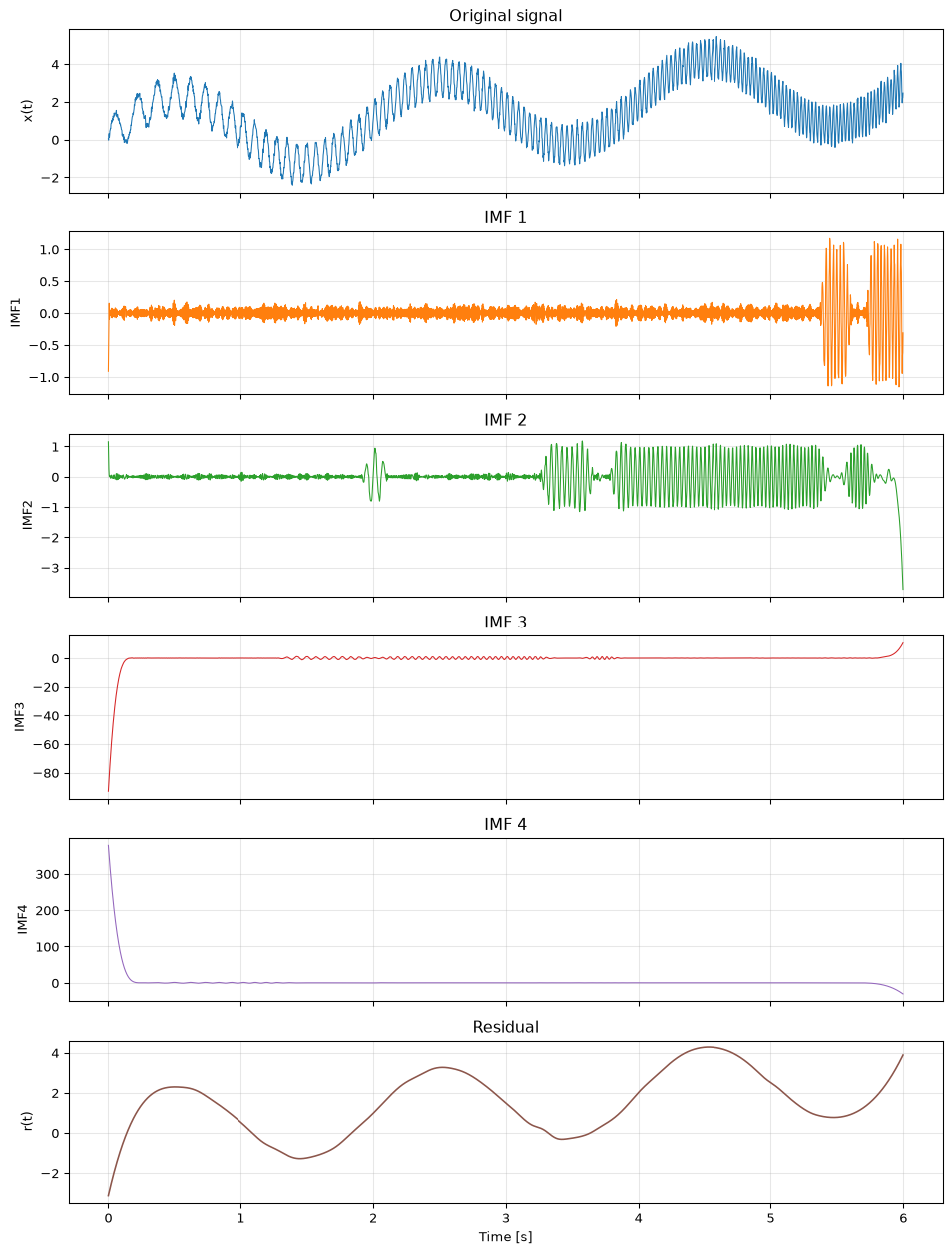
Advantages over Fourier
EMD has genuine strengths for certain signal classes:
- Non-stationary signals. A Fourier transform gives you the average spectral content over the analysis window. EMD tracks frequency changes within the signal because each IMF’s instantaneous frequency can vary with time.
- Nonlinear signals. Fourier assumes superposition: linear combinations of sinusoids. EMD makes no linearity assumption. Signals with frequency modulation, amplitude modulation, or nonlinear interactions can be decomposed into physically meaningful components.
- No basis selection. You do not need to choose a wavelet family, a window length, or a frequency grid. The decomposition adapts to the data.
Limitations
These are real, not minor caveats:
Mode mixing. When two components have similar frequencies or when a component has intermittent bursts, the sifting process can mix them into the same IMF or split one component across multiple IMFs. This is the single biggest practical problem with EMD. Ensemble EMD (EEMD) addresses this by averaging over many decompositions with added white noise, but it is computationally expensive and introduces its own parameters.
No mathematical foundation. EMD is an algorithm, not a transform. There is no inverse EMD, no uniqueness theorem, no convergence proof for the sifting process. The number of sifting iterations affects the result, and different stopping criteria give different IMFs. This makes it difficult to analyse theoretically or to make rigorous claims about the decomposition.
Boundary effects. The cubic spline interpolation for the envelopes is sensitive to the signal endpoints. Different endpoint handling strategies (mirror extension, extrapolation, clamping) give different results, especially for the lowest-frequency IMFs.
Sensitivity to noise. Adding even a small amount of noise can change the number and character of the IMFs. This is why EEMD adds noise deliberately, to exploit this sensitivity for more robust mode separation.
Variants
Several extensions have been proposed to address EMD’s limitations:
- EEMD (Ensemble EMD): adds white noise, decomposes many times, averages. Reduces mode mixing but is slow.
- CEEMDAN (Complete EEMD with Adaptive Noise): a refinement of EEMD that adds noise at each stage of decomposition. Better mode separation, still slow.
- VMD (Variational Mode Decomposition): formulates decomposition as an optimisation problem rather than a sifting process. Has a mathematical foundation but requires specifying the number of modes in advance.
For Python, the emd package (pip install emd) provides EEMD and other variants. The PyEMD package is another option. For VMD, see vmdpy.
When to use EMD
EMD is worth considering when:
- Your signal is genuinely non-stationary and you need to track frequency changes over time
- You do not know the number of components or their frequency ranges in advance
- Short-time Fourier transform or wavelets give unsatisfactory time-frequency resolution
EMD is not a good choice when:
- The signal is stationary or nearly so (just use Fourier analysis)
- You need reproducible, theoretically grounded results (use wavelets or parametric methods)
- You have a model for the signal components (use model-based decomposition instead)
Open questions
Mathematical foundations. Despite over 25 years of use, EMD still lacks a rigorous mathematical framework. Attempts to formalise it, through optimisation (VMD), synchrosqueezing, or operator theory, have produced related but distinct methods rather than a foundation for EMD itself. Whether EMD can ever be fully formalised, or whether it is inherently heuristic, remains open.
Stopping criteria. When should sifting stop? The original paper used a Cauchy-type criterion on successive differences, but the choice of threshold affects the resulting IMFs. More recent work uses energy-based or orthogonality-based criteria, but there is no consensus on the best approach.
Multivariate EMD. Extending EMD to vector-valued signals (e.g., multi-channel EEG) is non-trivial. The concept of “envelope” does not generalise naturally to multiple dimensions. Several multivariate variants exist (MEMD, NA-MEMD) but the field is still evolving.
References
Cobb, Kim M., Christopher D. Charles, Hai Cheng, and R. Lawrence Edwards. 2003. “El Niño/Southern Oscillation and Tropical Pacific Climate During the Last Millennium.” Nature 424: 271–76.
Huang, Norden E., Zheng Shen, Steven R. Long, Manli C. Wu, Hsing H. Shih, Quanan Zheng, Nai-Chyuan Yen, Chi Chao Tung, and Henry H. Liu. 1998. “The Empirical Mode Decomposition and the Hilbert Spectrum for Nonlinear and Non-Stationary Time Series Analysis.” Proceedings of the Royal Society of London A 454 (1971): 903–95. https://doi.org/10.1098/rspa.1998.0193.