The Short-Time Fourier Transform makes one decision and lives with it for the whole signal: the frame length. A long frame resolves closely-spaced frequencies but blurs the moment things change; a short frame catches the transient but cannot tell two nearby tones apart. The tiles on its time-frequency plane are all the same shape, and you pick that shape once, up front.
Real signals are not so considerate. A heartbeat is a slow baseline wander with sharp spikes riding on top; a music recording is sustained notes punctuated by percussive attacks; a fault in a bearing is a low rumble plus a brief click. Each mixes slow, frequency-precise content with fast, time-precise content, and no single frame length serves both.
The wavelet transform stops insisting on one tile shape. It analyses the signal with a family of waves that are all the same shape but different widths: wide ones for low frequencies (good frequency resolution, poor time resolution) and narrow ones for high frequencies (good time resolution, poor frequency resolution). The tiles get short and fat at the top of the band and tall and thin at the bottom. This is exactly the trade-off most signals want, because fast events tend to be brief and slow events tend to persist. The transform stops imposing one measure on everything and meets each event on its own terms: the fleeting briefly, the enduring at length.
This page builds directly on the STFT (the fixed-tiling baseline it improves on) and on multirate systems (downsampling and filter banks, the engine of the discrete transform).
Code
The implementation is wavelets.py. Save test_wavelets.py beside it and pytest test_wavelets.py runs the checks on it. It is hand-rolled from the filter coefficients up, with no external wavelet library, so every step is visible; in production you would reach for PyWavelets. One naming caveat if you port across: this page follows Daubechies’ tap-count convention, so its db4 is the four-tap, two-vanishing-moment wavelet, which PyWavelets calls db2 (PyWavelets indexes by vanishing moments, so its db4 is a different eight-tap wavelet).
Two transforms, two jobs
There are two wavelet transforms, and they answer different questions.
The continuous wavelet transform (CWT) is for looking. It correlates the signal with scaled, shifted copies of one mother wavelet at many overlapping scales, producing a redundant, finely-sampled scalogram. It is the wavelet analogue of the spectrogram, and the right tool for seeing where in time and scale the action is (Grossmann and Morlet 1984).
The discrete wavelet transform (DWT) is for working. It samples scale and position on a critical, non-redundant dyadic grid (powers of two), computed as a cascade of filter banks. It is perfectly invertible with exactly as many coefficients as input samples, which is what compression, denoising, and fast computation need (Mallat 1989).
This page takes the CWT first (to build the picture), then the DWT (to do the work).
The continuous transform: a scalogram
The CWT measures how much the signal looks like a wavelet \(\psi\) placed at time \(\tau\) and stretched by a scale \(s\):
The mother wavelet used here is the Morlet: a complex sinusoid under a Gaussian envelope, \(\psi(t) = \pi^{-1/4} e^{i \omega_0 t} e^{-t^2/2}\). It is the wavelet of choice for analysis because its envelope is as compact in time and frequency as the uncertainty principle allows, the same Gaussian-window optimum the STFT’s Gabor limit is built on. The difference is the \(1/s\) stretch: large \(s\) widens the wavelet for low frequencies, small \(s\) narrows it for high ones. Bigger scale means lower frequency, related by \(f \approx \omega_0 f_s / (2\pi s)\).
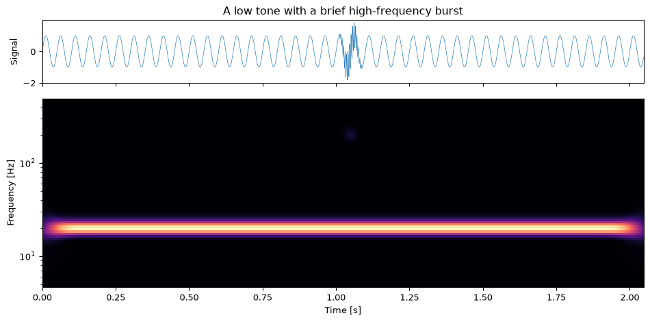
Here is the scalogram of a signal that defeats a single STFT frame: a steady low tone with a brief high-frequency burst buried inside it.
Show the code
fs, N =1000.0, 2048t = np.arange(N) / fslow = np.sin(2* np.pi *20* t) # a persistent low toneb0, b1 =1000, 1100# a brief 200 Hz burstburst = np.zeros(N)burst[b0:b1] = np.sin(2* np.pi *200* t[b0:b1]) * np.hanning(b1 - b0)x = low + burstscales = np.geomspace(2, 200, 80)freqs = cwt_frequencies(scales, fs)power = np.abs(cwt(x, scales)) **2fig, (a0, a1) = plt.subplots(2, 1, figsize=(10, 5), sharex=True, gridspec_kw={'height_ratios': [1, 3]})a0.plot(t, x, 'C0', lw=0.5); a0.set_ylabel('Signal')a0.set_title('A low tone with a brief high-frequency burst')a1.pcolormesh(t, freqs, power, shading='auto', cmap='magma')a1.set_yscale('log'); a1.set_ylabel('Frequency [Hz]'); a1.set_xlabel('Time [s]')fig.tight_layout(); plt.show()# the high band localises the burst in time; the low band runs the whole signalhi = power[np.argmin(np.abs(freqs -200))]lo = power[np.argmin(np.abs(freqs -20))]hi_peak_t = t[np.argmax(hi)]hi_support = np.sum(hi >0.5* hi.max()) # samples above half-maxlo_support = np.sum(lo >0.5* lo.max())assertabs(hi_peak_t -1.05) <0.02# burst found at 1.05 sassert hi_support <0.1* lo_support # burst is tightly localisedprint(f"200 Hz band: peak at {hi_peak_t:.3f} s, energy spread {hi_support} samples")print(f" 20 Hz band: energy spread {lo_support} samples (runs the whole signal)")
Figure 1: Scalogram (CWT magnitude) of a 20 Hz tone carrying a short 200 Hz burst at 1.05 s. The low tone shows as a horizontal band running the whole duration; the burst shows as a compact blob localised in both time and frequency. One transform resolves the persistent low tone and pins the brief high event, which no single STFT frame length can do at once.
200 Hz band: peak at 1.050 s, energy spread 36 samples
 20 Hz band: energy spread 1999 samples (runs the whole signal)
The low tone fills a thin horizontal band across the full duration: precise in frequency, deliberately vague in time, because a steady tone has no “when”. The burst is a compact patch: precise in time, broader in frequency. The wavelet gave each what it needed from the same analysis, with no frame-length knob to set.
Why the STFT cannot do this in one pass
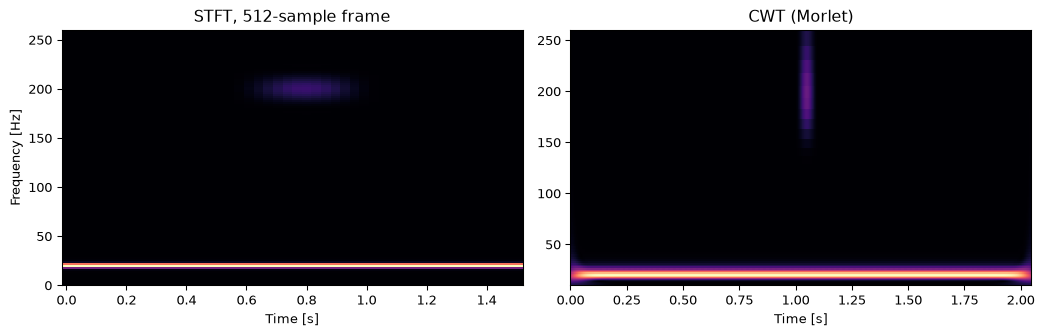
To resolve the 20 Hz tone, an STFT needs a long frame (tens of cycles, hundreds of milliseconds). But a long frame smears the 0.1 s burst across its whole width. Shorten the frame to pin the burst and the 20 Hz line dissolves. The wavelet escapes the dilemma by using a different effective window length at each frequency.
Show the code
def stft_mag(x, win, hop): w = np.hanning(win) starts =range(0, len(x) - win, hop)return np.stack([np.abs(np.fft.rfft(x[s:s + win] * w)) for s in starts], axis=1)win, hop =512, 32# ~0.5 s frame: resolves 20 HzS = stft_mag(x, win, hop)sf = np.fft.rfftfreq(win, 1/ fs)st_t = np.arange(S.shape[1]) * hop / fsfig, (a0, a1) = plt.subplots(1, 2, figsize=(11, 3.6), sharey=False)a0.pcolormesh(st_t, sf, S, shading='auto', cmap='magma')a0.set_ylim(0, 260); a0.set_title(f'STFT, {win}-sample frame')a0.set_xlabel('Time [s]'); a0.set_ylabel('Frequency [Hz]')a1.pcolormesh(t, freqs, np.sqrt(power), shading='auto', cmap='magma')a1.set_ylim(10, 260); a1.set_title('CWT (Morlet)')a1.set_xlabel('Time [s]')fig.tight_layout(); plt.show()# measure the burst's time spread at 200 Hz in each transformst_row = S[np.argmin(np.abs(sf -200))]st_support_s = np.sum(st_row >0.5* st_row.max()) * hop / fscwt_support_s = hi_support / fsassert cwt_support_s < st_support_s # wavelet is tighter in timeprint(f"burst time spread at 200 Hz: STFT {st_support_s*1000:.0f} ms, "f"CWT {cwt_support_s*1000:.0f} ms")
Figure 2: The 200 Hz burst as seen by an STFT with a frame long enough to resolve the 20 Hz tone (left) versus the CWT (right). The long STFT frame spreads the burst across its whole width; the wavelet, using a short effective window at high frequency, keeps it compact.
burst time spread at 200 Hz: STFT 256 ms, CWT 36 ms
The discrete transform: a tree of filter banks
The scalogram is a beautiful picture and a terrible data structure: it is hugely redundant, storing a value at every scale and every sample. For computation you want the discrete wavelet transform, which samples scale and position just densely enough to lose nothing and no more.
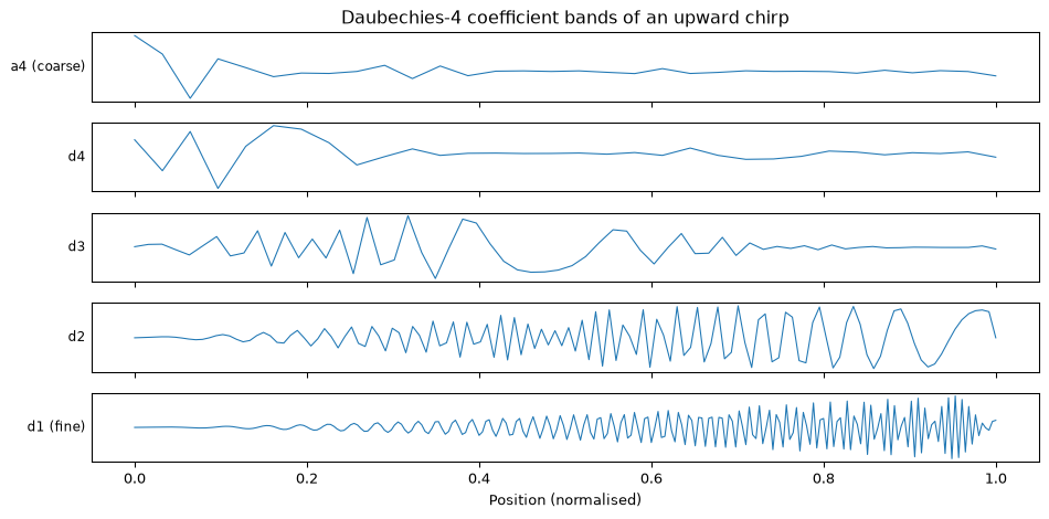
Mallat’s insight was that the DWT is a two-channel filter bank, recursed(Mallat 1989). At each level you split the signal into a low-pass (approximation) and high-pass (detail) half-band with a quadrature-mirror filter pair, then downsample each by two. The detail coefficients are kept; the approximation is fed back in and split again. Because each level halves the sample rate, this is precisely the multirate machinery, run as a tree:
with \(h\) the low-pass (scaling) filter and \(g\) its high-pass (wavelet) mirror. Run it \(J\) levels and you get one coarse approximation \(a_J\) plus detail bands \(d_J, \dots, d_1\), finest last. The whole transform is \(O(N)\), cheaper than the FFT’s \(O(N \log N)\), and because the filter pair is orthonormal it inverts exactly: synthesis upsamples each band and applies the same filters (for this page’s periodic, circular-convolution DWT the orthogonal inverse uses the identical coefficients with no time reversal; the standard linear-convolution form instead uses the time-reversed synthesis filters).
Show the code
n =512tt = np.linspace(0, 1, n, endpoint=False)chirp = np.sin(2* np.pi * (5+60* tt) * tt) # sweeps upwardcoeffs = wavedec(chirp, 'db4', level=4)labels = ['a4 (coarse)', 'd4', 'd3', 'd2', 'd1 (fine)']fig, axes = plt.subplots(len(coeffs), 1, figsize=(10, 5), sharex=True)for ax, c, lab inzip(axes, coeffs, labels): ax.plot(np.linspace(0, 1, len(c)), c, 'C0', lw=0.8) ax.set_ylabel(lab, rotation=0, ha='right', va='center', fontsize=9) ax.set_yticks([])axes[-1].set_xlabel('Position (normalised)')axes[0].set_title('Daubechies-4 coefficient bands of an upward chirp')fig.tight_layout(); plt.show()# perfect reconstruction: the orthonormal transform inverts exactlyrec = waverec(coeffs, 'db4')err = np.max(np.abs(rec - chirp))assert err <1e-12# energy is conserved across the bands (Parseval for an orthonormal basis)coeff_energy =sum(np.sum(c **2) for c in coeffs)assert np.isclose(coeff_energy, np.sum(chirp **2))print(f"reconstruction error {err:.1e}; coefficient energy matches signal energy")
Figure 3: A four-level Daubechies-4 decomposition of a chirp, shown as its coefficient bands (coarse approximation on top, finest detail at the bottom). Each finer detail band has twice the samples of the one above it and covers the next octave up; the coarse approximation a4 has the same length as the coarsest detail d4. Reconstructing from these coefficients returns the original to floating-point precision.
reconstruction error 1.7e-15; coefficient energy matches signal energy
Notice how the chirp’s energy walks from the coarse bands toward the fine ones as it sweeps up in frequency: the detail level a coefficient lives in is its octave.
Why this matters: energy compaction
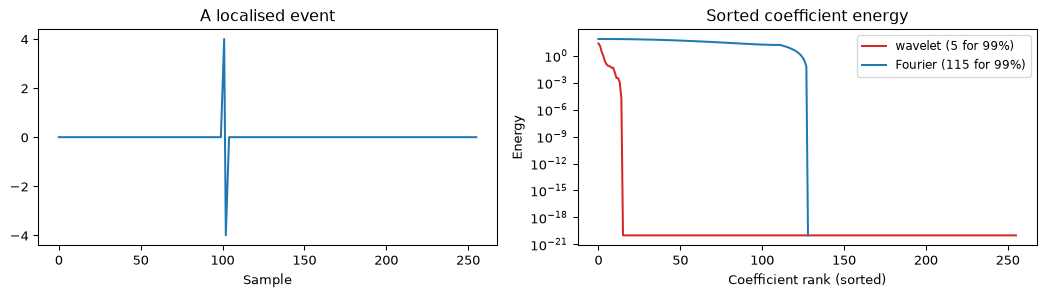
The reason the DWT underpins compression and denoising is that for signals with localised features it is sparse: a few large coefficients carry almost all the energy, and the rest are near zero. The Fourier transform of the same localised event spreads its energy across every bin, because a global sinusoid basis has to build a local bump out of broad waves that cancel everywhere else. Lining the two representations up side by side is the cleanest way to see why a localised basis wins.
Show the code
N =256event = np.zeros(N)event[100:104] = [2.0, 4.0, -4.0, -2.0] # a short, sharp featurecf = wavedec(event, 'db4', level=4)wave_coeffs = np.concatenate(cf)fft_coeffs = np.abs(np.fft.rfft(event))def n_for_99pct(energy_sorted):return np.searchsorted(np.cumsum(energy_sorted), 0.99* energy_sorted.sum()) +1n_wave = n_for_99pct(np.sort(wave_coeffs **2)[::-1])n_fft = n_for_99pct(np.sort(fft_coeffs **2)[::-1])fig, (a0, a1) = plt.subplots(1, 2, figsize=(11, 3.2))a0.plot(event, 'C0'); a0.set_title('A localised event'); a0.set_xlabel('Sample')a1.semilogy(np.sort(wave_coeffs **2)[::-1] +1e-20, 'C3', label=f'wavelet ({n_wave} for 99%)')a1.semilogy(np.sort(fft_coeffs **2)[::-1] +1e-20, 'C0', label=f'Fourier ({n_fft} for 99%)')a1.set_title('Sorted coefficient energy'); a1.set_xlabel('Coefficient rank (sorted)')a1.set_ylabel('Energy'); a1.legend(fontsize=9)fig.tight_layout(); plt.show()assert n_wave < n_fft # wavelet is the sparser basisprint(f"to hold 99% of the energy: {n_wave} wavelet coefficients vs {n_fft} Fourier")
Figure 4: A single localised event and the two ways to represent it. The wavelet (Daubechies-4) concentrates 99% of the energy into a handful of coefficients; the Fourier transform needs many more, because a localised bump is expensive to build from global sinusoids.
to hold 99% of the energy: 5 wavelet coefficients vs 115 Fourier
The families
A wavelet is defined by its filter pair, and the choice is a trade between time localisation, smoothness, and the number of vanishing moments (how many polynomial trends the detail filter ignores, which sets how sparse the transform is on smooth signals). Two orthonormal families are built into this page; the easiest way to see their shape is to inverse-transform a single nonzero detail coefficient, which reconstructs the wavelet itself.
Show the code
def wavelet_shape(name, N=128, level=4): c = wavedec(np.zeros(N), name, level) c[1] = np.zeros_like(c[1]); c[1][len(c[1]) //2] =1.0# one detail spikereturn waverec(c, name)fig, axes = plt.subplots(1, 3, figsize=(11, 3))axes[0].plot(wavelet_shape('haar'), 'C0'); axes[0].set_title('Haar (1 vanishing moment)')axes[1].plot(wavelet_shape('db4'), 'C0'); axes[1].set_title('Daubechies-4 (2 moments)')m = morlet(256, scale=16.0)axes[2].plot(m.real, 'C0', label='real'); axes[2].plot(m.imag, 'C3', lw=0.8, label='imag')axes[2].set_title('Morlet (for the CWT)'); axes[2].legend(fontsize=8)for ax in axes: ax.set_yticks([]); ax.set_xlabel('Sample')fig.tight_layout(); plt.show()# Daubechies-4 has two vanishing moments: its detail filter kills constant and# linear trends, which Haar's single moment does not_, g = wavelet_filters('db4')k = np.arange(len(g))assert np.isclose(np.sum(g), 0.0) and np.isclose(np.sum(k * g), 0.0)print("Daubechies-4 detail filter annihilates constant and linear trends")
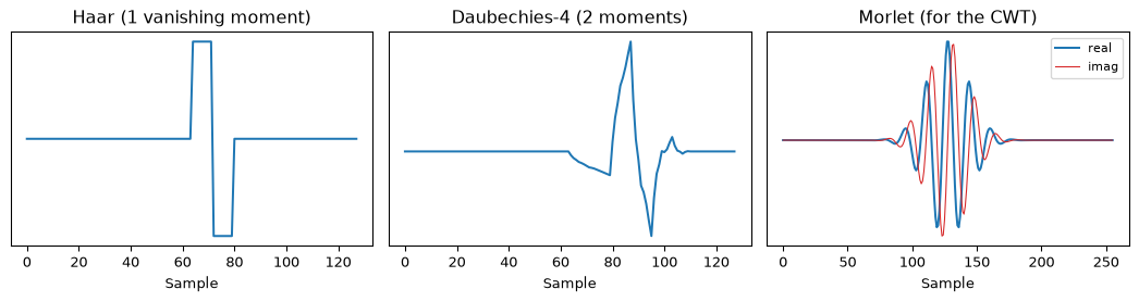
Figure 5: The Haar and Daubechies-4 wavelets (recovered by inverse-transforming one detail coefficient) and the Morlet wavelet used for the CWT. Haar is one square step: maximally compact but discontinuous. Daubechies-4 is wider and smoother with two vanishing moments. Morlet is a smooth, oscillatory, complex wavelet, ideal for analysis but not critically sampled.
Daubechies-4 detail filter annihilates constant and linear trends
Haar is the original wavelet: an average and a difference, perfectly localised in time but blocky and discontinuous, so it represents smooth signals poorly. Daubechies built the family that fixes this, the shortest orthonormal wavelets with a given number of vanishing moments (Daubechies 1992); Daubechies-4 (four taps, two vanishing moments) is the workhorse first step up from Haar. Morlet is not used for the DWT at all (it is not orthogonal and does not give critical sampling), but its smoothness makes it the standard analysis wavelet for the CWT.
Denoising: the headline application
Wavelet shrinkage is the application that made wavelets famous outside mathematics (Donoho 1995). The logic is the energy compaction above, turned into an algorithm. Transform the noisy signal; the signal’s features land in a few large coefficients while white noise spreads thinly across all of them at a roughly uniform level. So threshold: shrink every small detail coefficient toward zero, keep the large ones, and invert. The signal survives; most of the noise does not.
The threshold that makes this principled is the universal threshold\(\lambda = \sigma\sqrt{2 \ln N}\) (Donoho and Johnstone (Donoho and Johnstone 1994)), the level below which \(N\) samples of pure Gaussian noise almost surely fall. The noise scale \(\sigma\) is estimated robustly from the finest detail band, where signal is sparse, as \(\text{median}(|d_1|)/0.6745\).
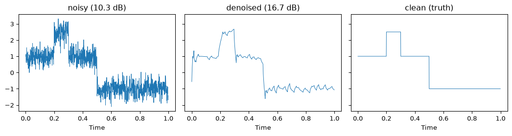
Figure 6: Wavelet shrinkage on a piecewise-constant signal in heavy noise. Soft-thresholding the Daubechies-4 detail coefficients removes most of the noise while keeping the sharp edges that a linear low-pass filter would round off.
SNR: 10.3 dB noisy -> 16.7 dB denoised
The edges stay crisp. That is the wavelet’s selling point over a low-pass filter, which would have to choose between passing the noise or blurring the steps; the wavelet keeps the edges because an edge is a localised event that lands in a few large, above-threshold detail coefficients.
The wavelet as a matched filter: finding the QRS complex
Denoising used the DWT to work. The CWT can also detect, and seeing why closes a loop with another topic. Read the transform’s defining inner product literally: \(W(s,\tau)\) correlates the signal with a wavelet placed at \(\tau\) and stretched to scale \(s\), and correlation against a known shape is exactly a matched filter. So when the wavelet at some scale is shaped like the event you are hunting, the CWT at that scale is the matched-filter response and its peaks mark the event.
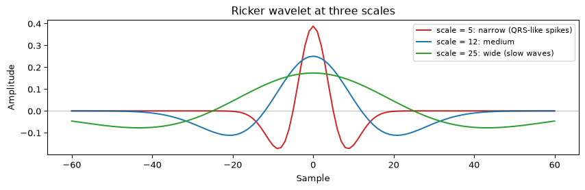
The clinical example is the QRS complex, the sharp spike of each heartbeat in an ECG. Its shape (a small dip, a tall narrow peak, another dip) is close to the Ricker wavelet, the Mexican hat: the negated second derivative of a Gaussian, one positive lobe flanked by two negative ones. At the scale whose central lobe is about as wide as a QRS, the Ricker is a QRS template.
Figure 7: The Ricker (Mexican hat) wavelet at three scales. A narrow one matches a sharp spike like the QRS; a wide one matches a slow wave. Convolving a signal with the wavelet at a given scale is a matched filter for features of that width.
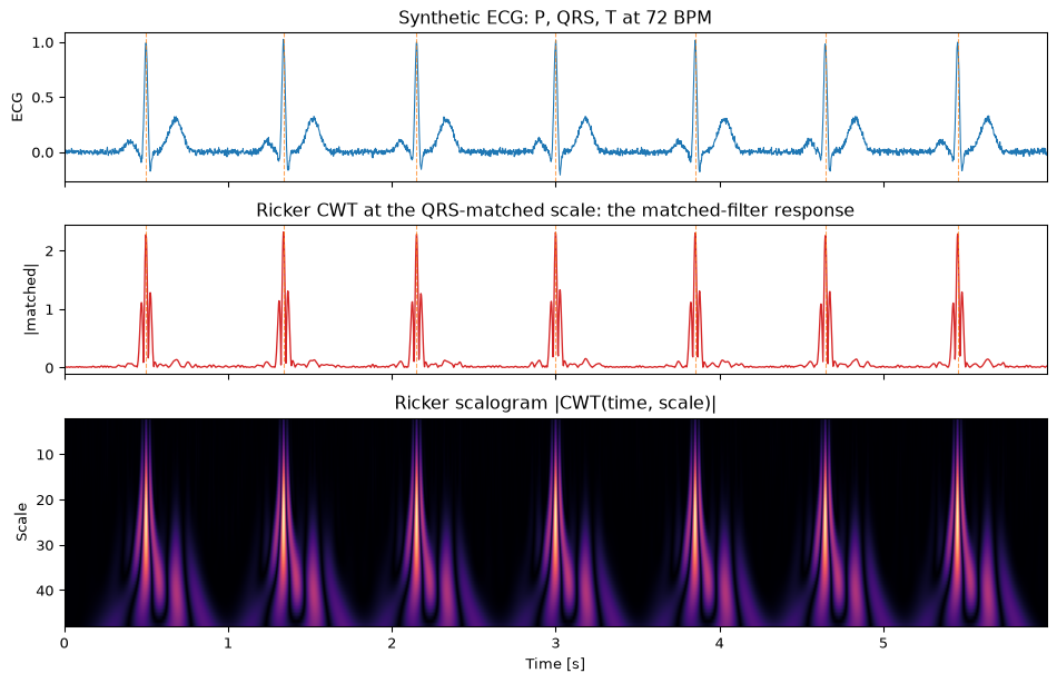
Slide that template across a synthetic ECG. The matched-filter response is the CWT magnitude at the QRS-matched scale, its peaks are the R-peaks, and the full scalogram shows the QRS energy concentrating in a narrow band of small scales while the slower P and T waves spread into wider ones.
Show the code
from scipy.signal import find_peaksfs, duration =500.0, 6.0N =int(fs * duration); t = np.arange(N) / fsrng = np.random.default_rng(42)beat_period =60.0/72# 72 BPMbeat_times = []; cur =0.5while cur < duration: beat_times.append(cur); cur += beat_period + rng.normal(0, 0.02)beat_times = np.array(beat_times)# Each beat is a sum of Gaussians at P, Q, R, S, T offsets. This is a# signal-shape ECG, not a physiological model; the R spike dominates.components = [(-0.100, 0.025, 0.10), (-0.025, 0.008, -0.10), (0.000, 0.010, 1.00), ( 0.025, 0.008, -0.20), ( 0.180, 0.040, 0.30)]ecg = np.zeros(N)for tb in beat_times:for off, sig, amp in components: ecg += amp * np.exp(-((t - (tb + off)) **2) / (2* sig **2))ecg +=0.015* rng.standard_normal(N)# Full scalogram, plus the single QRS-matched scale used for detection.scales = np.geomspace(2, 48, 60)coefs = np.abs(ricker_cwt(ecg, scales))qrs_scale =6.0# central lobe ~= QRS widthresponse = np.abs(ricker_cwt(ecg, [qrs_scale])[0])# Peak-pick the response: a height floor rejects noise, a 300 ms minimum# distance enforces the physiological refractory period (<= 200 BPM).peaks, _ = find_peaks(response, height=0.4* response.max(), distance=int(0.3* fs))assertlen(peaks) ==len(beat_times) # every beat found, no extrasprint(f"true beats: {len(beat_times)}, R-peaks detected: {len(peaks)}")fig, ax = plt.subplots(3, 1, figsize=(10, 6.5), sharex=True, gridspec_kw={'height_ratios': [1, 1, 1.4]})ax[0].plot(t, ecg, 'C0', lw=0.8); ax[0].set_ylabel('ECG')ax[0].set_title('Synthetic ECG: P, QRS, T at 72 BPM')ax[1].plot(t, response, 'C3', lw=1.0); ax[1].set_ylabel('|matched|')ax[1].set_title('Ricker CWT at the QRS-matched scale: the matched-filter response')for p in peaks: ax[0].axvline(p / fs, color='C1', ls='--', lw=0.8, alpha=0.7) ax[1].axvline(p / fs, color='C1', ls='--', lw=0.8, alpha=0.7)ax[2].imshow(coefs, aspect='auto', cmap='magma', origin='upper', extent=[t[0], t[-1], scales[-1], scales[0]])ax[2].set_ylabel('Scale'); ax[2].set_xlabel('Time [s]')ax[2].set_title('Ricker scalogram |CWT(time, scale)|')fig.tight_layout(); plt.show()
true beats: 7, R-peaks detected: 7
Figure 8: Wavelet QRS detection. Top: a synthetic ECG. Middle: the Ricker CWT magnitude at the QRS-matched scale, the matched-filter response, with detected R-peaks marked. Bottom: the scalogram; the QRS spikes light up a narrow band of small scales. Every one of the seven beats is recovered.
This is why wavelet-based QRS detectors are a standard tool: Li, Zheng and Tai reported over 99.8% detection on the MIT/BIH database using a wavelet across several scales (Li, Zheng, and Tai 1995). The single Mexican hat at one scale here is the teaching idealisation; production detectors use a quadratic-spline or Daubechies wavelet over a few dyadic scales with modulus-maxima matching, which is more robust to baseline wander and noise. Either way the principle is the one from matched filtering: when you know the shape, correlate for it.
And the output feeds forward. Once the R-peaks give you the sequence of inter-beat intervals, the heart-rate variability analysis on the PPG page takes over: detection finds the beats, an anomaly measure judges the rhythm. Same toolbox, two questions.
Going further
The lifting scheme. The filter-bank tree can be factored into a sequence of predict and update steps that work in place, need half the arithmetic, and can be made exactly invertible in integer arithmetic (Sweldens 1998). That is the form to reach for on a microcontroller, and it is the subject of the hardware page.
Wavelet packets. The DWT only recurses on the low-pass branch. Recurse on both and you get a wavelet packet tree, a richer (and adaptive) tiling of the time-frequency plane that can match a signal’s structure more closely, at more cost.
The constant-Q and scattering transforms. The CWT’s logarithmic frequency spacing is the constant-Q transform under another name, which is why it suits music. Cascading wavelet transforms with modulus nonlinearities gives the scattering transform, a stable, translation-invariant feature front end that behaves like the first layers of a convolutional network.
It is not a spectrogram. A scalogram’s axis is scale (log-frequency), not linear frequency, and its tiles change shape with frequency. Reading it like an STFT spectrogram is the commonest beginner error. When you want fixed linear-frequency tiles, the STFT is still the right tool; wavelets win when the interesting events live at very different timescales. For a fully data-driven decomposition that picks no basis at all, see empirical mode decomposition.
References
Daubechies, Ingrid. 1992. Ten Lectures on Wavelets. CBMS-NSF Regional Conference Series in Applied Mathematics 61. Society for Industrial; Applied Mathematics (SIAM).
Donoho, David L. 1995. “De-Noising by Soft-Thresholding.”IEEE Transactions on Information Theory 41 (3): 613–27.
Donoho, David L., and Iain M. Johnstone. 1994. “Ideal Spatial Adaptation by Wavelet Shrinkage.”Biometrika 81 (3): 425–55.
Grossmann, Alexander, and Jean Morlet. 1984. “Decomposition of Hardy Functions into Square Integrable Wavelets of Constant Shape.”SIAM Journal on Mathematical Analysis 15 (4): 723–36.
Li, Cuiwei, Chongxun Zheng, and Changfeng Tai. 1995. “Detection of ECG Characteristic Points Using Wavelet Transforms.”IEEE Transactions on Biomedical Engineering 42 (1): 21–28. https://doi.org/10.1109/10.362922.
Mallat, Stéphane G. 1989. “A Theory for Multiresolution Signal Decomposition: The Wavelet Representation.”IEEE Transactions on Pattern Analysis and Machine Intelligence 11 (7): 674–93.
Sweldens, Wim. 1998. “The Lifting Scheme: A Construction of Second Generation Wavelets.”SIAM Journal on Mathematical Analysis 29 (2): 511–46.
Source Code
---title: "Wavelets"subtitle: "When one window size is not enough"description-meta: "When one window size is not enough: wavelet analysis tiles time and frequency adaptively, unlike the fixed frames of the STFT."bibliography: ../../references.bib---The [Short-Time Fourier Transform](../stft/index.qmd) makes one decision and lives with it for the whole signal: the frame length. A long frame resolves closely-spaced frequencies but blurs the moment things change; a short frame catches the transient but cannot tell two nearby tones apart. The tiles on its time-frequency plane are all the same shape, and you pick that shape once, up front.Real signals are not so considerate. A heartbeat is a slow baseline wander with sharp spikes riding on top; a music recording is sustained notes punctuated by percussive attacks; a fault in a bearing is a low rumble plus a brief click. Each mixes slow, frequency-precise content with fast, time-precise content, and no single frame length serves both.The **wavelet transform** stops insisting on one tile shape. It analyses the signal with a family of waves that are all the same shape but **different widths**: wide ones for low frequencies (good frequency resolution, poor time resolution) and narrow ones for high frequencies (good time resolution, poor frequency resolution). The tiles get short and fat at the top of the band and tall and thin at the bottom. This is exactly the trade-off most signals want, because fast events tend to be brief and slow events tend to persist. The transform stops imposing one measure on everything and meets each event on its own terms: the fleeting briefly, the enduring at length.::: {.callout-note title="Prerequisites"}Part of the [feature extraction arc](../feature-extraction.qmd); the overview gives the reading order.This page builds directly on the [STFT](../stft/index.qmd) (the fixed-tiling baseline it improves on) and on [multirate systems](../../basics/10-multirate/index.qmd) (downsampling and filter banks, the engine of the discrete transform).:::::: {.callout-tip title="Code"}The implementation is [`wavelets.py`](wavelets.py). Save [`test_wavelets.py`](test_wavelets.py) beside it and `pytest test_wavelets.py` runs the checks on it. It is hand-rolled from the filter coefficients up, with no external wavelet library, so every step is visible; in production you would reach for [PyWavelets](https://pywavelets.readthedocs.io). One naming caveat if you port across: this page follows Daubechies' tap-count convention, so its `db4` is the four-tap, two-vanishing-moment wavelet, which PyWavelets calls `db2` (PyWavelets indexes by vanishing moments, so its `db4` is a different eight-tap wavelet).:::```{python}#| echo: falseimport numpy as npimport matplotlib.pyplot as pltfrom wavelets import (cwt, cwt_frequencies, morlet, ricker, ricker_cwt, wavelet_filters, wavedec, waverec, denoise)```## Two transforms, two jobsThere are two wavelet transforms, and they answer different questions.- The **continuous wavelet transform (CWT)** is for *looking*. It correlates the signal with scaled, shifted copies of one mother wavelet at many overlapping scales, producing a redundant, finely-sampled **scalogram**. It is the wavelet analogue of the spectrogram, and the right tool for seeing where in time and scale the action is [@grossmann1984decomposition].- The **discrete wavelet transform (DWT)** is for *working*. It samples scale and position on a critical, non-redundant dyadic grid (powers of two), computed as a cascade of filter banks. It is perfectly invertible with exactly as many coefficients as input samples, which is what compression, denoising, and fast computation need [@mallat1989theory].This page takes the CWT first (to build the picture), then the DWT (to do the work).## The continuous transform: a scalogramThe CWT measures how much the signal looks like a wavelet $\psi$ placed at time $\tau$ and stretched by a scale $s$:$$W(s, \tau) = \frac{1}{\sqrt{s}} \int x(t)\, \psi^{*}\!\left(\frac{t - \tau}{s}\right) dt$$The mother wavelet used here is the **Morlet**: a complex sinusoid under a Gaussian envelope, $\psi(t) = \pi^{-1/4} e^{i \omega_0 t} e^{-t^2/2}$. It is the wavelet of choice for analysis because its envelope is as compact in time and frequency as the uncertainty principle allows, the same Gaussian-window optimum the [STFT's Gabor limit](../stft/index.qmd) is built on. The difference is the $1/s$ stretch: large $s$ widens the wavelet for low frequencies, small $s$ narrows it for high ones. Bigger scale means lower frequency, related by $f \approx \omega_0 f_s / (2\pi s)$.Here is the scalogram of a signal that defeats a single STFT frame: a steady low tone with a brief high-frequency burst buried inside it.```{python}#| label: fig-scalogram#| fig-cap: "Scalogram (CWT magnitude) of a 20 Hz tone carrying a short 200 Hz burst at 1.05 s. The low tone shows as a horizontal band running the whole duration; the burst shows as a compact blob localised in both time and frequency. One transform resolves the persistent low tone *and* pins the brief high event, which no single STFT frame length can do at once."#| code-fold: truefs, N =1000.0, 2048t = np.arange(N) / fslow = np.sin(2* np.pi *20* t) # a persistent low toneb0, b1 =1000, 1100# a brief 200 Hz burstburst = np.zeros(N)burst[b0:b1] = np.sin(2* np.pi *200* t[b0:b1]) * np.hanning(b1 - b0)x = low + burstscales = np.geomspace(2, 200, 80)freqs = cwt_frequencies(scales, fs)power = np.abs(cwt(x, scales)) **2fig, (a0, a1) = plt.subplots(2, 1, figsize=(10, 5), sharex=True, gridspec_kw={'height_ratios': [1, 3]})a0.plot(t, x, 'C0', lw=0.5); a0.set_ylabel('Signal')a0.set_title('A low tone with a brief high-frequency burst')a1.pcolormesh(t, freqs, power, shading='auto', cmap='magma')a1.set_yscale('log'); a1.set_ylabel('Frequency [Hz]'); a1.set_xlabel('Time [s]')fig.tight_layout(); plt.show()# the high band localises the burst in time; the low band runs the whole signalhi = power[np.argmin(np.abs(freqs -200))]lo = power[np.argmin(np.abs(freqs -20))]hi_peak_t = t[np.argmax(hi)]hi_support = np.sum(hi >0.5* hi.max()) # samples above half-maxlo_support = np.sum(lo >0.5* lo.max())assertabs(hi_peak_t -1.05) <0.02# burst found at 1.05 sassert hi_support <0.1* lo_support # burst is tightly localisedprint(f"200 Hz band: peak at {hi_peak_t:.3f} s, energy spread {hi_support} samples")print(f" 20 Hz band: energy spread {lo_support} samples (runs the whole signal)")```The low tone fills a thin horizontal band across the full duration: precise in frequency, deliberately vague in time, because a steady tone has no "when". The burst is a compact patch: precise in time, broader in frequency. The wavelet gave each what it needed from the same analysis, with no frame-length knob to set.## Why the STFT cannot do this in one passTo resolve the 20 Hz tone, an STFT needs a long frame (tens of cycles, hundreds of milliseconds). But a long frame smears the 0.1 s burst across its whole width. Shorten the frame to pin the burst and the 20 Hz line dissolves. The wavelet escapes the dilemma by using a *different* effective window length at each frequency.```{python}#| label: fig-stft-vs-wavelet#| fig-cap: "The 200 Hz burst as seen by an STFT with a frame long enough to resolve the 20 Hz tone (left) versus the CWT (right). The long STFT frame spreads the burst across its whole width; the wavelet, using a short effective window at high frequency, keeps it compact."#| code-fold: truedef stft_mag(x, win, hop): w = np.hanning(win) starts =range(0, len(x) - win, hop)return np.stack([np.abs(np.fft.rfft(x[s:s + win] * w)) for s in starts], axis=1)win, hop =512, 32# ~0.5 s frame: resolves 20 HzS = stft_mag(x, win, hop)sf = np.fft.rfftfreq(win, 1/ fs)st_t = np.arange(S.shape[1]) * hop / fsfig, (a0, a1) = plt.subplots(1, 2, figsize=(11, 3.6), sharey=False)a0.pcolormesh(st_t, sf, S, shading='auto', cmap='magma')a0.set_ylim(0, 260); a0.set_title(f'STFT, {win}-sample frame')a0.set_xlabel('Time [s]'); a0.set_ylabel('Frequency [Hz]')a1.pcolormesh(t, freqs, np.sqrt(power), shading='auto', cmap='magma')a1.set_ylim(10, 260); a1.set_title('CWT (Morlet)')a1.set_xlabel('Time [s]')fig.tight_layout(); plt.show()# measure the burst's time spread at 200 Hz in each transformst_row = S[np.argmin(np.abs(sf -200))]st_support_s = np.sum(st_row >0.5* st_row.max()) * hop / fscwt_support_s = hi_support / fsassert cwt_support_s < st_support_s # wavelet is tighter in timeprint(f"burst time spread at 200 Hz: STFT {st_support_s*1000:.0f} ms, "f"CWT {cwt_support_s*1000:.0f} ms")```## The discrete transform: a tree of filter banksThe scalogram is a beautiful picture and a terrible data structure: it is hugely redundant, storing a value at every scale and every sample. For computation you want the **discrete wavelet transform**, which samples scale and position just densely enough to lose nothing and no more.Mallat's insight was that the DWT is a **two-channel filter bank, recursed** [@mallat1989theory]. At each level you split the signal into a low-pass (approximation) and high-pass (detail) half-band with a quadrature-mirror filter pair, then downsample each by two. The detail coefficients are kept; the approximation is fed back in and split again. Because each level halves the sample rate, this is precisely the [multirate](../../basics/10-multirate/index.qmd) machinery, run as a tree:$$x \to \boxed{h, \downarrow 2} \to a_1 \to \boxed{h, \downarrow 2} \to a_2 \to \cdots \qquad x \to \boxed{g, \downarrow 2} \to d_1$$with $h$ the low-pass (scaling) filter and $g$ its high-pass (wavelet) mirror. Run it $J$ levels and you get one coarse approximation $a_J$ plus detail bands $d_J, \dots, d_1$, finest last. The whole transform is $O(N)$, cheaper than the FFT's $O(N \log N)$, and because the filter pair is orthonormal it inverts exactly: synthesis upsamples each band and applies the same filters (for this page's periodic, circular-convolution DWT the orthogonal inverse uses the identical coefficients with no time reversal; the standard linear-convolution form instead uses the time-reversed synthesis filters).```{python}#| label: fig-pr#| fig-cap: "A four-level Daubechies-4 decomposition of a chirp, shown as its coefficient bands (coarse approximation on top, finest detail at the bottom). Each finer detail band has twice the samples of the one above it and covers the next octave up; the coarse approximation a4 has the same length as the coarsest detail d4. Reconstructing from these coefficients returns the original to floating-point precision."#| code-fold: truen =512tt = np.linspace(0, 1, n, endpoint=False)chirp = np.sin(2* np.pi * (5+60* tt) * tt) # sweeps upwardcoeffs = wavedec(chirp, 'db4', level=4)labels = ['a4 (coarse)', 'd4', 'd3', 'd2', 'd1 (fine)']fig, axes = plt.subplots(len(coeffs), 1, figsize=(10, 5), sharex=True)for ax, c, lab inzip(axes, coeffs, labels): ax.plot(np.linspace(0, 1, len(c)), c, 'C0', lw=0.8) ax.set_ylabel(lab, rotation=0, ha='right', va='center', fontsize=9) ax.set_yticks([])axes[-1].set_xlabel('Position (normalised)')axes[0].set_title('Daubechies-4 coefficient bands of an upward chirp')fig.tight_layout(); plt.show()# perfect reconstruction: the orthonormal transform inverts exactlyrec = waverec(coeffs, 'db4')err = np.max(np.abs(rec - chirp))assert err <1e-12# energy is conserved across the bands (Parseval for an orthonormal basis)coeff_energy =sum(np.sum(c **2) for c in coeffs)assert np.isclose(coeff_energy, np.sum(chirp **2))print(f"reconstruction error {err:.1e}; coefficient energy matches signal energy")```Notice how the chirp's energy walks from the coarse bands toward the fine ones as it sweeps up in frequency: the detail level a coefficient lives in *is* its octave.## Why this matters: energy compactionThe reason the DWT underpins compression and denoising is that for signals with localised features it is **sparse**: a few large coefficients carry almost all the energy, and the rest are near zero. The Fourier transform of the same localised event spreads its energy across every bin, because a global sinusoid basis has to build a local bump out of broad waves that cancel everywhere else. Lining the two representations up side by side is the cleanest way to see why a localised basis wins.```{python}#| label: fig-compaction#| fig-cap: "A single localised event and the two ways to represent it. The wavelet (Daubechies-4) concentrates 99% of the energy into a handful of coefficients; the Fourier transform needs many more, because a localised bump is expensive to build from global sinusoids."#| code-fold: trueN =256event = np.zeros(N)event[100:104] = [2.0, 4.0, -4.0, -2.0] # a short, sharp featurecf = wavedec(event, 'db4', level=4)wave_coeffs = np.concatenate(cf)fft_coeffs = np.abs(np.fft.rfft(event))def n_for_99pct(energy_sorted):return np.searchsorted(np.cumsum(energy_sorted), 0.99* energy_sorted.sum()) +1n_wave = n_for_99pct(np.sort(wave_coeffs **2)[::-1])n_fft = n_for_99pct(np.sort(fft_coeffs **2)[::-1])fig, (a0, a1) = plt.subplots(1, 2, figsize=(11, 3.2))a0.plot(event, 'C0'); a0.set_title('A localised event'); a0.set_xlabel('Sample')a1.semilogy(np.sort(wave_coeffs **2)[::-1] +1e-20, 'C3', label=f'wavelet ({n_wave} for 99%)')a1.semilogy(np.sort(fft_coeffs **2)[::-1] +1e-20, 'C0', label=f'Fourier ({n_fft} for 99%)')a1.set_title('Sorted coefficient energy'); a1.set_xlabel('Coefficient rank (sorted)')a1.set_ylabel('Energy'); a1.legend(fontsize=9)fig.tight_layout(); plt.show()assert n_wave < n_fft # wavelet is the sparser basisprint(f"to hold 99% of the energy: {n_wave} wavelet coefficients vs {n_fft} Fourier")```## The familiesA wavelet is defined by its filter pair, and the choice is a trade between time localisation, smoothness, and the number of **vanishing moments** (how many polynomial trends the detail filter ignores, which sets how sparse the transform is on smooth signals). Two orthonormal families are built into this page; the easiest way to see their shape is to inverse-transform a single nonzero detail coefficient, which reconstructs the wavelet itself.```{python}#| label: fig-families#| fig-cap: "The Haar and Daubechies-4 wavelets (recovered by inverse-transforming one detail coefficient) and the Morlet wavelet used for the CWT. Haar is one square step: maximally compact but discontinuous. Daubechies-4 is wider and smoother with two vanishing moments. Morlet is a smooth, oscillatory, complex wavelet, ideal for analysis but not critically sampled."#| code-fold: truedef wavelet_shape(name, N=128, level=4): c = wavedec(np.zeros(N), name, level) c[1] = np.zeros_like(c[1]); c[1][len(c[1]) //2] =1.0# one detail spikereturn waverec(c, name)fig, axes = plt.subplots(1, 3, figsize=(11, 3))axes[0].plot(wavelet_shape('haar'), 'C0'); axes[0].set_title('Haar (1 vanishing moment)')axes[1].plot(wavelet_shape('db4'), 'C0'); axes[1].set_title('Daubechies-4 (2 moments)')m = morlet(256, scale=16.0)axes[2].plot(m.real, 'C0', label='real'); axes[2].plot(m.imag, 'C3', lw=0.8, label='imag')axes[2].set_title('Morlet (for the CWT)'); axes[2].legend(fontsize=8)for ax in axes: ax.set_yticks([]); ax.set_xlabel('Sample')fig.tight_layout(); plt.show()# Daubechies-4 has two vanishing moments: its detail filter kills constant and# linear trends, which Haar's single moment does not_, g = wavelet_filters('db4')k = np.arange(len(g))assert np.isclose(np.sum(g), 0.0) and np.isclose(np.sum(k * g), 0.0)print("Daubechies-4 detail filter annihilates constant and linear trends")```Haar is the original wavelet: an average and a difference, perfectly localised in time but blocky and discontinuous, so it represents smooth signals poorly. Daubechies built the family that fixes this, the shortest orthonormal wavelets with a given number of vanishing moments [@daubechies1992ten]; Daubechies-4 (four taps, two vanishing moments) is the workhorse first step up from Haar. Morlet is not used for the DWT at all (it is not orthogonal and does not give critical sampling), but its smoothness makes it the standard analysis wavelet for the CWT.## Denoising: the headline applicationWavelet shrinkage is the application that made wavelets famous outside mathematics [@donoho1995denoising]. The logic is the energy compaction above, turned into an algorithm. Transform the noisy signal; the signal's features land in a few large coefficients while white noise spreads thinly across all of them at a roughly uniform level. So **threshold**: shrink every small detail coefficient toward zero, keep the large ones, and invert. The signal survives; most of the noise does not.The threshold that makes this principled is the **universal threshold** $\lambda = \sigma\sqrt{2 \ln N}$ (Donoho and Johnstone [@donohojohnstone1994]), the level below which $N$ samples of pure Gaussian noise almost surely fall. The noise scale $\sigma$ is estimated robustly from the finest detail band, where signal is sparse, as $\text{median}(|d_1|)/0.6745$.```{python}#| label: fig-denoise#| fig-cap: "Wavelet shrinkage on a piecewise-constant signal in heavy noise. Soft-thresholding the Daubechies-4 detail coefficients removes most of the noise while keeping the sharp edges that a linear low-pass filter would round off."#| code-fold: truerng = np.random.default_rng(7)M =1024tt = np.linspace(0, 1, M, endpoint=False)clean = np.where(tt <0.5, 1.0, -1.0) + np.where((tt >0.2) & (tt <0.3), 1.5, 0.0)noisy = clean +0.4* rng.standard_normal(M)out = denoise(noisy, 'db4', level=4)def snr(est):return10* np.log10(np.sum(clean **2) / np.sum((est - clean) **2))fig, axes = plt.subplots(1, 3, figsize=(11, 3), sharey=True)for ax, sig, name in [(axes[0], noisy, f'noisy ({snr(noisy):.1f} dB)'), (axes[1], out, f'denoised ({snr(out):.1f} dB)'), (axes[2], clean, 'clean (truth)')]: ax.plot(tt, sig, 'C0', lw=0.7); ax.set_title(name); ax.set_xlabel('Time')fig.tight_layout(); plt.show()assert snr(out) > snr(noisy) +3# at least 3 dB cleanerprint(f"SNR: {snr(noisy):.1f} dB noisy -> {snr(out):.1f} dB denoised")```The edges stay crisp. That is the wavelet's selling point over a low-pass filter, which would have to choose between passing the noise or blurring the steps; the wavelet keeps the edges because an edge is a localised event that lands in a few large, above-threshold detail coefficients.## The wavelet as a matched filter: finding the QRS complex {#wavelet-matched-filter}Denoising used the DWT to *work*. The CWT can also *detect*, and seeing why closes a loop with another topic. Read the transform's defining inner product literally: $W(s,\tau)$ correlates the signal with a wavelet placed at $\tau$ and stretched to scale $s$, and correlation against a known shape is exactly a [matched filter](../matched-filtering/index.qmd). So when the wavelet at some scale is shaped like the event you are hunting, the CWT at that scale *is* the matched-filter response and its peaks mark the event.The clinical example is the **QRS complex**, the sharp spike of each heartbeat in an ECG. Its shape (a small dip, a tall narrow peak, another dip) is close to the **Ricker wavelet**, the Mexican hat: the negated second derivative of a Gaussian, one positive lobe flanked by two negative ones. At the scale whose central lobe is about as wide as a QRS, the Ricker is a QRS template.```{python}#| label: fig-ricker-basis#| fig-cap: "The Ricker (Mexican hat) wavelet at three scales. A narrow one matches a sharp spike like the QRS; a wide one matches a slow wave. Convolving a signal with the wavelet at a given scale is a matched filter for features of that width."#| code-fold: truett = np.arange(-60, 61)fig, ax = plt.subplots(figsize=(9, 3))for s, c, lbl inzip([5, 12, 25], ['C3', 'C0', 'C2'], ['narrow (QRS-like spikes)', 'medium', 'wide (slow waves)']): ax.plot(tt, ricker(len(tt), s), c, label=f'scale = {s}: {lbl}')ax.axhline(0, color='k', lw=0.5, alpha=0.4)ax.set_xlabel('Sample'); ax.set_ylabel('Amplitude')ax.set_title('Ricker wavelet at three scales'); ax.legend(fontsize=8)fig.tight_layout(); plt.show()```Slide that template across a synthetic ECG. The matched-filter response is the CWT magnitude at the QRS-matched scale, its peaks are the R-peaks, and the full scalogram shows the QRS energy concentrating in a narrow band of small scales while the slower P and T waves spread into wider ones.```{python}#| label: fig-qrs#| fig-cap: "Wavelet QRS detection. Top: a synthetic ECG. Middle: the Ricker CWT magnitude at the QRS-matched scale, the matched-filter response, with detected R-peaks marked. Bottom: the scalogram; the QRS spikes light up a narrow band of small scales. Every one of the seven beats is recovered."#| code-fold: truefrom scipy.signal import find_peaksfs, duration =500.0, 6.0N =int(fs * duration); t = np.arange(N) / fsrng = np.random.default_rng(42)beat_period =60.0/72# 72 BPMbeat_times = []; cur =0.5while cur < duration: beat_times.append(cur); cur += beat_period + rng.normal(0, 0.02)beat_times = np.array(beat_times)# Each beat is a sum of Gaussians at P, Q, R, S, T offsets. This is a# signal-shape ECG, not a physiological model; the R spike dominates.components = [(-0.100, 0.025, 0.10), (-0.025, 0.008, -0.10), (0.000, 0.010, 1.00), ( 0.025, 0.008, -0.20), ( 0.180, 0.040, 0.30)]ecg = np.zeros(N)for tb in beat_times:for off, sig, amp in components: ecg += amp * np.exp(-((t - (tb + off)) **2) / (2* sig **2))ecg +=0.015* rng.standard_normal(N)# Full scalogram, plus the single QRS-matched scale used for detection.scales = np.geomspace(2, 48, 60)coefs = np.abs(ricker_cwt(ecg, scales))qrs_scale =6.0# central lobe ~= QRS widthresponse = np.abs(ricker_cwt(ecg, [qrs_scale])[0])# Peak-pick the response: a height floor rejects noise, a 300 ms minimum# distance enforces the physiological refractory period (<= 200 BPM).peaks, _ = find_peaks(response, height=0.4* response.max(), distance=int(0.3* fs))assertlen(peaks) ==len(beat_times) # every beat found, no extrasprint(f"true beats: {len(beat_times)}, R-peaks detected: {len(peaks)}")fig, ax = plt.subplots(3, 1, figsize=(10, 6.5), sharex=True, gridspec_kw={'height_ratios': [1, 1, 1.4]})ax[0].plot(t, ecg, 'C0', lw=0.8); ax[0].set_ylabel('ECG')ax[0].set_title('Synthetic ECG: P, QRS, T at 72 BPM')ax[1].plot(t, response, 'C3', lw=1.0); ax[1].set_ylabel('|matched|')ax[1].set_title('Ricker CWT at the QRS-matched scale: the matched-filter response')for p in peaks: ax[0].axvline(p / fs, color='C1', ls='--', lw=0.8, alpha=0.7) ax[1].axvline(p / fs, color='C1', ls='--', lw=0.8, alpha=0.7)ax[2].imshow(coefs, aspect='auto', cmap='magma', origin='upper', extent=[t[0], t[-1], scales[-1], scales[0]])ax[2].set_ylabel('Scale'); ax[2].set_xlabel('Time [s]')ax[2].set_title('Ricker scalogram |CWT(time, scale)|')fig.tight_layout(); plt.show()```This is why wavelet-based QRS detectors are a standard tool: Li, Zheng and Tai reported over 99.8% detection on the MIT/BIH database using a wavelet across several scales [@li1995detection]. The single Mexican hat at one scale here is the teaching idealisation; production detectors use a quadratic-spline or Daubechies wavelet over a few dyadic scales with modulus-maxima matching, which is more robust to baseline wander and noise. Either way the principle is the one from [matched filtering](../matched-filtering/index.qmd): when you know the shape, correlate for it.And the output feeds forward. Once the R-peaks give you the sequence of inter-beat intervals, the [heart-rate variability analysis](../ppg/index.qmd#hrv-poincare) on the PPG page takes over: detection finds the beats, an anomaly measure judges the rhythm. Same toolbox, two questions.## Going further- **The lifting scheme.** The filter-bank tree can be factored into a sequence of *predict* and *update* steps that work in place, need half the arithmetic, and can be made exactly invertible in integer arithmetic [@sweldens1998lifting]. That is the form to reach for on a microcontroller, and it is the subject of the [hardware page](embedded.qmd).- **Wavelet packets.** The DWT only recurses on the low-pass branch. Recurse on *both* and you get a wavelet packet tree, a richer (and adaptive) tiling of the time-frequency plane that can match a signal's structure more closely, at more cost.- **The constant-Q and scattering transforms.** The CWT's logarithmic frequency spacing is the constant-Q transform under another name, which is why it suits music. Cascading wavelet transforms with modulus nonlinearities gives the *scattering transform*, a stable, translation-invariant feature front end that behaves like the first layers of a convolutional network.- **It is not a spectrogram.** A scalogram's axis is scale (log-frequency), not linear frequency, and its tiles change shape with frequency. Reading it like an STFT spectrogram is the commonest beginner error. When you want fixed linear-frequency tiles, the [STFT](../stft/index.qmd) is still the right tool; wavelets win when the interesting events live at very different timescales. For a fully data-driven decomposition that picks no basis at all, see [empirical mode decomposition](../emd/index.qmd).## References::: {#refs}:::