Estimating the fundamental frequency of speech and music: from autocorrelation to real-time embedded systems
When you hum a note, your vocal folds vibrate at a rate called the fundamental frequency (\(f_0\)). This single number (typically 85–255 Hz for speech, 27.5–4186 Hz for a piano) determines the perceived pitch. Estimating \(f_0\) from a recorded or streaming audio signal is one of the oldest problems in signal processing, and one that still generates research papers today.
The applications are everywhere: speech therapy systems that give real-time feedback on intonation, musical tuners that tell a guitarist whether their string is sharp or flat, voice assistants that distinguish questions from statements by tracking pitch contour, and singing training apps that score your performance against a reference melody. For the complete embedded implementation with I2S audio, BLE output, and performance budgets, see Pitch Detection on Hardware.
Despite decades of work, pitch detection remains surprisingly hard. The fundamental is often weaker than its harmonics. Background noise corrupts the signal. Voiced and unvoiced speech alternate rapidly. And in real-time systems, you need answers fast (within 20–40 ms) while keeping computational cost low enough for a microcontroller.
Biomimicry: how we hear pitch
The human auditory system uses two complementary mechanisms for pitch estimation. In the temporal pathway, auditory nerve fibres phase-lock to the stimulus waveform; their firing times encode the period of the signal, and the brain extracts pitch from the inter-spike intervals. In the spectral pathway, the cochlea acts as a bank of overlapping bandpass filters (the basilar membrane’s tonotopic map), and the brain infers \(f_0\) from the pattern of harmonics that are resolved. That filter bank is modelled explicitly in the gammatone filters topic. Both mechanisms contribute, with temporal cues dominating below ~1 kHz and spectral cues above ~4 kHz. This dual strategy inspired many computational pitch detectors that combine time-domain and frequency-domain estimates. (Robles and Ruggero 2001; see also Cheveigné 2005 for a comprehensive review)
The simplest pitch estimator counts zero crossings. If a periodic signal with fundamental frequency \(f_0\) is sampled at rate \(f_s\), the number of zero crossings per second is approximately \(2 f_0\) (one upward crossing and one downward crossing per period). The estimated pitch is:
\[\hat{f}_0 = \frac{Z}{2T}\]
where \(Z\) is the number of zero crossings in a window of duration \(T\) seconds.
This works for a pure sinusoid but breaks down for real speech, which contains harmonics. A vowel at 150 Hz has strong energy at 300, 450, 600 Hz and beyond; each harmonic adds zero crossings, biasing the estimate upward. Bandpass filtering the signal to the expected \(f_0\) range (e.g., 80–500 Hz) before counting crossings helps significantly, but the method remains fragile.
Autocorrelation method
A more robust approach exploits the periodicity of voiced speech directly. The autocorrelation function (ACF) of a periodic signal has peaks at lags equal to integer multiples of the period. The first peak after the zero-lag maximum gives the period estimate:
where \(\tau_\min\) corresponds to the maximum expected \(f_0\) (e.g., \(\tau_\min = f_s / 500\) for 500 Hz upper bound).
The autocorrelation method is far more robust to harmonics than zero-crossing rate because it responds to the periodicity of the waveform, not individual crossings. It is the basis of many practical pitch detectors.
import numpy as npimport matplotlib.pyplot as plt# Generate a synthetic vowel: f0 = 150 Hz with harmonicsfs =16000duration =0.05# 50 ms for visualizationt = np.arange(int(fs * duration)) / fsf0_true =150.0# Voiced speech approximation: fundamental + harmonics with decreasing amplitudeharmonics = [1, 2, 3, 4, 5, 6]amplitudes = [1.0, 0.8, 0.5, 0.3, 0.15, 0.08]signal = np.zeros_like(t)for h, a inzip(harmonics, amplitudes): signal += a * np.sin(2* np.pi * f0_true * h * t)# Longer signal for estimationdur_est =0.04# 40 ms analysis windown_est =int(fs * dur_est)t_est = np.arange(n_est) / fssig_est = np.zeros(n_est)for h, a inzip(harmonics, amplitudes): sig_est += a * np.sin(2* np.pi * f0_true * h * t_est)# Method 1: Zero-crossing ratecrossings = np.where(np.diff(np.sign(sig_est)))[0]zcr =len(crossings) / (2* dur_est)# Method 2: Autocorrelationacf = np.correlate(sig_est, sig_est, mode='full')acf = acf[len(sig_est) -1:] # keep positive lags onlyacf /= acf[0] # normalise# Find first peak after minimum lag (max f0 = 500 Hz)min_lag =int(fs /500)max_lag =int(fs /80)acf_search = acf[min_lag:max_lag]peak_lag = min_lag + np.argmax(acf_search)f0_acf = fs / peak_lagfig, axes = plt.subplots(1, 3, figsize=(12, 3.5))# Waveformaxes[0].plot(t *1000, signal[:len(t)], 'C0', linewidth=0.8)axes[0].set_xlabel('Time [ms]')axes[0].set_ylabel('Amplitude')axes[0].set_title('Synthetic vowel (f0 = 150 Hz)')axes[0].grid(True, alpha=0.3)# Autocorrelationlag_ms = np.arange(len(acf)) / fs *1000axes[1].plot(lag_ms[:max_lag +20], acf[:max_lag +20], 'C0', linewidth=0.8)axes[1].axvline(peak_lag / fs *1000, color='C3', linestyle='--', label=f'Peak at {peak_lag/fs*1000:.1f} ms → {f0_acf:.0f} Hz')axes[1].set_xlabel('Lag [ms]')axes[1].set_ylabel('Normalised ACF')axes[1].set_title('Autocorrelation method')axes[1].legend(fontsize=8)axes[1].grid(True, alpha=0.3)# Comparisonmethods = ['True f0', 'ZCR', 'ACF']values = [f0_true, zcr, f0_acf]colors = ['C2', 'C1', 'C3']bars = axes[2].bar(methods, values, color=colors, alpha=0.8)axes[2].set_ylabel('Frequency [Hz]')axes[2].set_title('Estimate comparison')for bar, val inzip(bars, values): axes[2].text(bar.get_x() + bar.get_width() /2, bar.get_height() +5,f'{val:.0f} Hz', ha='center', fontsize=9)axes[2].grid(True, alpha=0.3, axis='y')fig.tight_layout()plt.show()
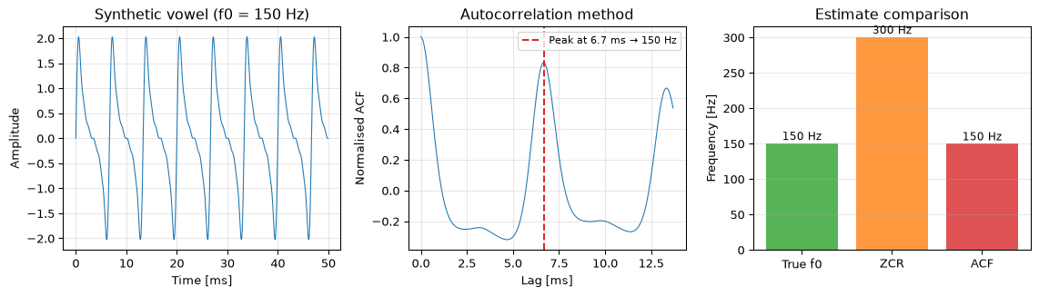
Figure 1: Time-domain pitch estimation on a synthetic vowel (f0 = 150 Hz). Zero-crossing rate overestimates pitch due to harmonics. The autocorrelation method finds the correct period.
The result speaks clearly: zero-crossing rate is led astray by the harmonics, while the autocorrelation method locks onto the correct period of 6.67 ms (150 Hz).
Frequency-domain methods
Periodogram peak detection
The most direct frequency-domain approach computes the power spectrum via FFT and finds the dominant peak in the speech band. For a windowed frame of \(N\) samples:
The pitch estimate is the frequency of the largest spectral peak within the expected \(f_0\) range:
\[\hat{f}_0 = \frac{f_s}{N} \arg\max_{k_\min \leq k \leq k_\max} P[k]\]
The frequency resolution is \(\Delta f = f_s / N\). For a 40 ms window at 16 kHz (\(N = 640\)), \(\Delta f = 25\) Hz, adequate for speech but not for precise musical tuning. Zero-padding improves the visual appearance of the spectrum but does not improve true resolution.
A critical limitation: the spectral peak method can lock onto a harmonic rather than the fundamental, especially when the first harmonic is stronger (common in male speech).
Harmonic product spectrum
The harmonic product spectrum (HPS) exploits the harmonic structure of voiced speech to find the fundamental even when it is weaker than its overtones. The idea: downsample the spectrum by factors 2, 3, …, \(H\) and multiply:
\[\text{HPS}[k] = \prod_{h=1}^{H} P[h \cdot k]\]
At the true fundamental \(k_0\), every downsampled version contributes a peak (since the \(h\)-th harmonic at \(h \cdot k_0\) maps to \(k_0\) after downsampling by \(h\)). At harmonics, only some terms align. The product thus amplifies the fundamental and suppresses harmonics.
import numpy as npimport matplotlib.pyplot as pltfs =16000duration =0.04# 40 ms windown_samples =int(fs * duration)t = np.arange(n_samples) / fsf0_true =150.0# Synthetic vowel where second harmonic is strongest (common in male speech)harmonics = [1, 2, 3, 4, 5, 6]amplitudes = [0.6, 1.0, 0.7, 0.4, 0.2, 0.1]signal = np.zeros(n_samples)for h, a inzip(harmonics, amplitudes): signal += a * np.sin(2* np.pi * f0_true * h * t)# Apply Hann windowwindow = np.hanning(n_samples)sig_win = signal * window# Zero-pad for smoother spectrumnfft =4096X = np.abs(np.fft.rfft(sig_win, n=nfft))freqs = np.fft.rfftfreq(nfft, 1/ fs)P = X **2# Periodogram peak in speech bandk_min =int(80* nfft / fs)k_max =int(500* nfft / fs)peak_k = k_min + np.argmax(P[k_min:k_max])f0_peak = freqs[peak_k]# Harmonic product spectrumH =5# number of harmonics to usehps = np.copy(P[:len(P)])for h inrange(2, H +1): decimated = P[::h] hps[:len(decimated)] *= decimatedhps_search = hps[k_min:k_max]hps_peak_k = k_min + np.argmax(hps_search)f0_hps = freqs[hps_peak_k]fig, axes = plt.subplots(1, 2, figsize=(11, 3.5))# Periodogramaxes[0].plot(freqs[:k_max +50], 10* np.log10(P[:k_max +50] / P.max() +1e-12),'C0', linewidth=0.8)axes[0].axvline(f0_peak, color='C1', linestyle='--', label=f'Peak: {f0_peak:.0f} Hz')axes[0].axvline(f0_true, color='C2', linestyle=':', alpha=0.7, label=f'True f0: {f0_true:.0f} Hz')axes[0].set_xlabel('Frequency [Hz]')axes[0].set_ylabel('Power [dB]')axes[0].set_title('Periodogram — locks onto 2nd harmonic')axes[0].legend(fontsize=8)axes[0].grid(True, alpha=0.3)# HPShps_db =10* np.log10(hps[:k_max +50] / hps[:k_max +50].max() +1e-12)axes[1].plot(freqs[:k_max +50], hps_db, 'C3', linewidth=0.8)axes[1].axvline(f0_hps, color='C3', linestyle='--', label=f'HPS peak: {f0_hps:.0f} Hz')axes[1].axvline(f0_true, color='C2', linestyle=':', alpha=0.7, label=f'True f0: {f0_true:.0f} Hz')axes[1].set_xlabel('Frequency [Hz]')axes[1].set_ylabel('Power [dB]')axes[1].set_title('Harmonic product spectrum — finds true f0')axes[1].legend(fontsize=8)axes[1].grid(True, alpha=0.3)fig.tight_layout()plt.show()
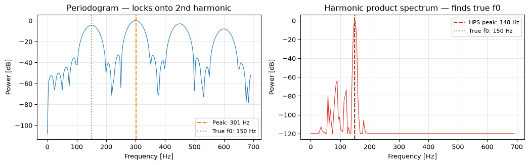
Figure 2: Frequency-domain pitch estimation. Left: the periodogram shows harmonics at 150, 300, 450, 600 Hz; the strongest peak is at 300 Hz (second harmonic). Right: the harmonic product spectrum correctly identifies 150 Hz as the fundamental.
The periodogram alone is fooled by the dominant second harmonic at 300 Hz. The harmonic product spectrum correctly identifies 150 Hz by exploiting the fact that all harmonics are integer multiples of the fundamental.
Voice activity detection
Before estimating pitch, you need to know when there is speech. Applying a pitch detector to silence, noise, or unvoiced consonants (like “s” or “f”) produces nonsense. Voice activity detection (VAD) answers a binary question: is the current frame voiced speech?
Three features, used together, give a simple but effective VAD:
Short-time energy. Voiced speech has significantly more power than background noise. Compute the RMS energy per frame and compare to a threshold. The threshold can be adaptive: set it at some multiple of the estimated noise floor.
Spectral centroid. Voiced speech concentrates energy in the low-frequency harmonics (below ~3 kHz). Unvoiced fricatives (“s”, “sh”) have their energy concentrated above 3 kHz. The spectral centroid is the power-weighted mean frequency:
\[f_c = \frac{\sum_k f_k \, P[k]}{\sum_k P[k]}\]
A low spectral centroid suggests voiced speech; a high one suggests noise or fricatives.
Zero-crossing rate. Voiced speech has a relatively low zero-crossing rate (dominated by the fundamental and low harmonics). Unvoiced speech and noise have high zero-crossing rates. This complements the energy feature: noise can have moderate energy but always has a high ZCR.
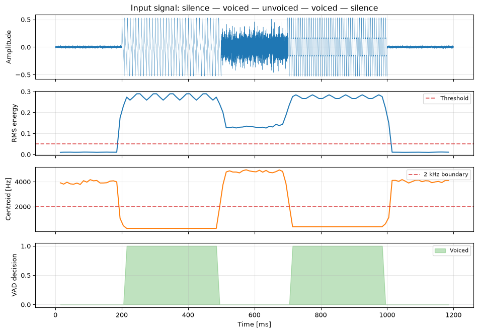
Figure 3: Voice activity detection using energy, spectral centroid, and zero-crossing rate. Voiced segments (vowels) have high energy, low spectral centroid, and low ZCR.
The VAD correctly identifies the two voiced segments while rejecting the silence and the unvoiced fricative. In practice, more sophisticated features (cepstral coefficients, learned classifiers) improve robustness, but these three simple features form the core of many embedded VAD systems.
Real-time considerations
Real-time pitch detection introduces constraints that offline analysis can ignore:
Block processing. Audio arrives in blocks (frames) from the ADC or I2S interface. Each frame is analysed independently or with overlap. Typical frame sizes:
Frame size
Duration at 16 kHz
Frequency resolution
Latency
256 samples
16 ms
62.5 Hz
Low, poor resolution
512 samples
32 ms
31.25 Hz
Good compromise
640 samples
40 ms
25 Hz
Good resolution, more latency
1024 samples
64 ms
15.6 Hz
High resolution, noticeable delay
The resolution-latency trade-off. Frequency resolution \(\Delta f = f_s / N\) improves with longer windows, but longer windows mean more latency. For speech at 100 Hz, you need at least 2 periods in the window: that is 20 ms minimum. In practice, 30–40 ms windows (480–640 samples at 16 kHz) give adequate resolution for speech with acceptable latency.
Overlap-add. To produce smooth pitch tracks, frames overlap by 50–75%. This gives a pitch estimate every 10 ms without sacrificing frequency resolution.
Computational budget. On a microcontroller, you may have only a few milliseconds of CPU time per frame. The autocorrelation method requires \(O(N^2)\) multiplications in the naive implementation, but restricting the lag search range (80–500 Hz) reduces this substantially. An FFT-based approach costs \(O(N \log N)\) and is often preferred when an FFT library is available.
The ESP32 implementation
The VoicePitchEstimator project implements real-time pitch estimation on an ESP32 microcontroller with an I2S MEMS microphone. The architecture follows the pipeline we have developed in this topic:
Figure 4: The VoicePitchEstimator pipeline: a bandpass biquad feeds a time-domain (ZCR), a spectral (FFT periodogram), and a voice-activity branch, fused into a pitch estimate sent over BLE.
Signal conditioning: biquad bandpass
The first processing step is a bandpass filter (80–500 Hz) implemented as a cascade of two second-order sections. This removes DC offset, low-frequency rumble, and high-frequency harmonics that would confuse the zero-crossing estimator. The biquad cascade is the standard structure for IIR filtering on embedded targets (see biquad filters for the theory).
// Biquad cascade: 2 second-order sections for bandpass 80-500 Hztypedefstruct{float b0, b1, b2, a1, a2;float x1, x2, y1, y2;// state variables} BiquadState;static BiquadState sos[2];// two sectionsfloat biquad_process(BiquadState *s,float x){float y = s->b0 * x + s->b1 * s->x1 + s->b2 * s->x2- s->a1 * s->y1 - s->a2 * s->y2; s->x2 = s->x1; s->x1 = x; s->y2 = s->y1; s->y1 = y;return y;}float bandpass_filter(float sample){float out = sample;for(int i =0; i <2; i++){ out = biquad_process(&sos[i], out);}return out;}
This uses Direct Form I (four state variables). The biquad topic compares this with the Transposed Direct Form II used in the PPG example.
Pitch estimation: ZCR + periodogram
The system uses two estimators in parallel. The zero-crossing rate gives a fast, cheap estimate that is accurate enough when the bandpass filter has removed most harmonics. The FFT periodogram provides a more reliable estimate at higher computational cost:
// Periodogram-based pitch detection on a 512-sample framevoid estimate_pitch_fft(float*frame,int n,float fs,float*f0_out,float*confidence){// Apply Hann windowfor(int i =0; i < n; i++) frame[i]*=0.5f*(1.0f- cosf(2.0f* M_PI * i /(n -1)));// Compute FFT (ESP32 DSP library provides dsps_fft2r_fc32)// ... FFT computation ...// Find peak in 80-500 Hz bandint k_min =(int)(80.0f* n / fs);int k_max =(int)(500.0f* n / fs);float max_power =0;int peak_bin = k_min;for(int k = k_min; k <= k_max; k++){float power = re[k]*re[k]+ im[k]*im[k];if(power > max_power){ max_power = power; peak_bin = k;}}*f0_out =(float)peak_bin * fs / n;// Confidence from peak-to-median ratio*confidence = max_power /(median_power +1e-10f);}
Voice activity detection
The VAD gate prevents the system from outputting pitch estimates during silence or unvoiced speech. It combines three criteria: power above a noise-floor threshold, spectral centroid within the voiced speech band, and spectral spread (second moment) below a limit that rejects broadband noise:
bool is_voiced(float power,float centroid,float spread,float zcr){return(power > noise_floor *3.0f)// enough energy&&(centroid >80.0f)// not pure DC/rumble&&(centroid <2000.0f)// not unvoiced fricative&&(spread <1500.0f)// not broadband noise&&(zcr <0.15f);// not noise/unvoiced}
The complete system runs on a single ESP32 core at 240 MHz, processing 512-sample frames at 16 kHz (32 ms per frame, ~10 ms computation time per frame), and transmits the pitch estimate over BLE for display on a connected device.
Open questions
Polyphonic pitch detection. Estimating multiple simultaneous \(f_0\) values (e.g., two singers, a chord on a guitar) remains hard. The harmonic series of different notes overlap and interact. Non-negative matrix factorisation and deep learning approaches show promise but are far too expensive for embedded targets.
Pitch in noise. All methods degrade in noise. The autocorrelation method is more robust than spectral peak detection, but still fails below ~0 dB SNR for speech. PYIN (Mauch and Dixon 2014) uses a probabilistic framework over multiple YIN candidates to improve tracking in noisy conditions.
Deep learning approaches. CREPE (Kim et al. 2018) uses a CNN trained on synthesised audio to estimate pitch directly from the waveform, achieving state-of-the-art accuracy. It is too large for microcontrollers but sets the benchmark for offline accuracy. Tiny versions for embedded deployment are an active research area.
Pitch tracking vs. pitch detection. A single-frame estimate is noisy. Tracking \(f_0\) over time (with continuity constraints, Viterbi decoding, or Kalman filtering) produces much smoother pitch contours. The trade-off between tracking smoothness and responsiveness to genuine pitch changes (vibrato, intonation) is still tuned by hand in most systems.
Octave errors. The most common failure mode: the detector jumps to \(2f_0\) or \(f_0/2\). Autocorrelation can produce a stronger peak at half the period (missing the true fundamental); spectral methods can lock onto a harmonic. Robust systems use multiple methods and cross-check.
Connections
Biquad filters: the bandpass pre-filter in the ESP32 implementation
Cheveigné, Alain de. 2005. “Pitch Perception Models.” In Pitch: Neural Coding and Perception, edited by Christopher J. Plack, Andrew J. Oxenham, Richard R. Fay, and Arthur N. Popper, 169–233. Springer. https://doi.org/10.1007/0-387-28958-5_6.
Kim, Jong Wook, Justin Salamon, Peter Li, and Juan Pablo Bello. 2018. “CREPE: A Convolutional Representation for Pitch Estimation.” In Proceedings of the IEEE International Conference on Acoustics, Speech and Signal Processing (ICASSP), 161–65. https://doi.org/10.1109/ICASSP.2018.8461329.
Mauch, Matthias, and Simon Dixon. 2014. “PYIN: A Fundamental Frequency Estimator Using Probabilistic Threshold Distributions.”Proceedings of the IEEE International Conference on Acoustics, Speech and Signal Processing (ICASSP), 659–63. https://doi.org/10.1109/ICASSP.2014.6853678.
Robles, Luis, and Mario A. Ruggero. 2001. “Mechanics of the Mammalian Cochlea.”Physiological Reviews 81 (3): 1305–52.
Source Code
---title: "Pitch Detection"subtitle: "Estimating the fundamental frequency of speech and music: from autocorrelation to real-time embedded systems"---When you hum a note, your vocal folds vibrate at a rate called the **fundamental frequency** ($f_0$). This single number (typically 85–255 Hz for speech, 27.5–4186 Hz for a piano) determines the perceived *pitch*. Estimating $f_0$ from a recorded or streaming audio signal is one of the oldest problems in signal processing, and one that still generates research papers today.The applications are everywhere: speech therapy systems that give real-time feedback on intonation, musical tuners that tell a guitarist whether their string is sharp or flat, voice assistants that distinguish questions from statements by tracking pitch contour, and singing training apps that score your performance against a reference melody. For the complete embedded implementation with I2S audio, BLE output, and performance budgets, see [Pitch Detection on Hardware](embedded.qmd).Despite decades of work, pitch detection remains surprisingly hard. The fundamental is often weaker than its harmonics. Background noise corrupts the signal. Voiced and unvoiced speech alternate rapidly. And in real-time systems, you need answers fast (within 20–40 ms) while keeping computational cost low enough for a microcontroller.::: {.callout-note title="Biomimicry: how we hear pitch"}The human auditory system uses two complementary mechanisms for pitch estimation. In the **temporal** pathway, auditory nerve fibres phase-lock to the stimulus waveform; their firing times encode the period of the signal, and the brain extracts pitch from the inter-spike intervals. In the **spectral** pathway, the cochlea acts as a bank of overlapping bandpass filters (the basilar membrane's tonotopic map), and the brain infers $f_0$ from the pattern of harmonics that are resolved. That filter bank is modelled explicitly in the [gammatone filters](../gammatone-filters/index.qmd) topic. Both mechanisms contribute, with temporal cues dominating below ~1 kHz and spectral cues above ~4 kHz. This dual strategy inspired many computational pitch detectors that combine time-domain and frequency-domain estimates. [@robles2001mechanics; see also @dechevigne2005pitch for a comprehensive review]:::::: {.callout-note title="Prerequisites"}This topic assumes familiarity with the [frequency domain](../../basics/05-frequency-domain.qmd) (DFT, periodogram, frequency resolution). Background on [biquad filters](../biquad/index.qmd) and [zero-crossing detection](../zero-crossing/index.qmd) is helpful but not required.:::---## Time-domain methods### Zero-crossing rateThe simplest pitch estimator counts zero crossings. If a periodic signal with fundamental frequency $f_0$ is sampled at rate $f_s$, the number of zero crossings per second is approximately $2 f_0$ (one upward crossing and one downward crossing per period). The estimated pitch is:$$\hat{f}_0 = \frac{Z}{2T}$$where $Z$ is the number of zero crossings in a window of duration $T$ seconds.This works for a pure sinusoid but breaks down for real speech, which contains harmonics. A vowel at 150 Hz has strong energy at 300, 450, 600 Hz and beyond; each harmonic adds zero crossings, biasing the estimate upward. Bandpass filtering the signal to the expected $f_0$ range (e.g., 80–500 Hz) before counting crossings helps significantly, but the method remains fragile.### Autocorrelation methodA more robust approach exploits the periodicity of voiced speech directly. The **autocorrelation function** (ACF) of a periodic signal has peaks at lags equal to integer multiples of the period. The first peak after the zero-lag maximum gives the period estimate:$$\hat{T}_0 = \arg\max_{\tau > \tau_\min} R_{xx}[\tau]$$$$\hat{f}_0 = \frac{f_s}{\hat{T}_0}$$where $\tau_\min$ corresponds to the maximum expected $f_0$ (e.g., $\tau_\min = f_s / 500$ for 500 Hz upper bound).The autocorrelation method is far more robust to harmonics than zero-crossing rate because it responds to the *periodicity* of the waveform, not individual crossings. It is the basis of many practical pitch detectors.```{python}#| label: fig-pitch-time-domain#| fig-cap: "Time-domain pitch estimation on a synthetic vowel (f0 = 150 Hz). Zero-crossing rate overestimates pitch due to harmonics. The autocorrelation method finds the correct period."import numpy as npimport matplotlib.pyplot as plt# Generate a synthetic vowel: f0 = 150 Hz with harmonicsfs =16000duration =0.05# 50 ms for visualizationt = np.arange(int(fs * duration)) / fsf0_true =150.0# Voiced speech approximation: fundamental + harmonics with decreasing amplitudeharmonics = [1, 2, 3, 4, 5, 6]amplitudes = [1.0, 0.8, 0.5, 0.3, 0.15, 0.08]signal = np.zeros_like(t)for h, a inzip(harmonics, amplitudes): signal += a * np.sin(2* np.pi * f0_true * h * t)# Longer signal for estimationdur_est =0.04# 40 ms analysis windown_est =int(fs * dur_est)t_est = np.arange(n_est) / fssig_est = np.zeros(n_est)for h, a inzip(harmonics, amplitudes): sig_est += a * np.sin(2* np.pi * f0_true * h * t_est)# Method 1: Zero-crossing ratecrossings = np.where(np.diff(np.sign(sig_est)))[0]zcr =len(crossings) / (2* dur_est)# Method 2: Autocorrelationacf = np.correlate(sig_est, sig_est, mode='full')acf = acf[len(sig_est) -1:] # keep positive lags onlyacf /= acf[0] # normalise# Find first peak after minimum lag (max f0 = 500 Hz)min_lag =int(fs /500)max_lag =int(fs /80)acf_search = acf[min_lag:max_lag]peak_lag = min_lag + np.argmax(acf_search)f0_acf = fs / peak_lagfig, axes = plt.subplots(1, 3, figsize=(12, 3.5))# Waveformaxes[0].plot(t *1000, signal[:len(t)], 'C0', linewidth=0.8)axes[0].set_xlabel('Time [ms]')axes[0].set_ylabel('Amplitude')axes[0].set_title('Synthetic vowel (f0 = 150 Hz)')axes[0].grid(True, alpha=0.3)# Autocorrelationlag_ms = np.arange(len(acf)) / fs *1000axes[1].plot(lag_ms[:max_lag +20], acf[:max_lag +20], 'C0', linewidth=0.8)axes[1].axvline(peak_lag / fs *1000, color='C3', linestyle='--', label=f'Peak at {peak_lag/fs*1000:.1f} ms → {f0_acf:.0f} Hz')axes[1].set_xlabel('Lag [ms]')axes[1].set_ylabel('Normalised ACF')axes[1].set_title('Autocorrelation method')axes[1].legend(fontsize=8)axes[1].grid(True, alpha=0.3)# Comparisonmethods = ['True f0', 'ZCR', 'ACF']values = [f0_true, zcr, f0_acf]colors = ['C2', 'C1', 'C3']bars = axes[2].bar(methods, values, color=colors, alpha=0.8)axes[2].set_ylabel('Frequency [Hz]')axes[2].set_title('Estimate comparison')for bar, val inzip(bars, values): axes[2].text(bar.get_x() + bar.get_width() /2, bar.get_height() +5,f'{val:.0f} Hz', ha='center', fontsize=9)axes[2].grid(True, alpha=0.3, axis='y')fig.tight_layout()plt.show()```The result speaks clearly: zero-crossing rate is led astray by the harmonics, while the autocorrelation method locks onto the correct period of 6.67 ms (150 Hz).---## Frequency-domain methods### Periodogram peak detectionThe most direct frequency-domain approach computes the power spectrum via FFT and finds the dominant peak in the speech band. For a windowed frame of $N$ samples:$$P[k] = \frac{1}{N} |X[k]|^2, \qquad X[k] = \sum_{n=0}^{N-1} x[n] \, w[n] \, e^{-j2\pi kn/N}$$The pitch estimate is the frequency of the largest spectral peak within the expected $f_0$ range:$$\hat{f}_0 = \frac{f_s}{N} \arg\max_{k_\min \leq k \leq k_\max} P[k]$$The frequency resolution is $\Delta f = f_s / N$. For a 40 ms window at 16 kHz ($N = 640$), $\Delta f = 25$ Hz, adequate for speech but not for precise musical tuning. Zero-padding improves the visual appearance of the spectrum but does not improve true resolution.A critical limitation: the spectral peak method can lock onto a harmonic rather than the fundamental, especially when the first harmonic is stronger (common in male speech).### Harmonic product spectrumThe **harmonic product spectrum** (HPS) exploits the harmonic structure of voiced speech to find the fundamental even when it is weaker than its overtones. The idea: downsample the spectrum by factors 2, 3, ..., $H$ and multiply:$$\text{HPS}[k] = \prod_{h=1}^{H} P[h \cdot k]$$At the true fundamental $k_0$, every downsampled version contributes a peak (since the $h$-th harmonic at $h \cdot k_0$ maps to $k_0$ after downsampling by $h$). At harmonics, only some terms align. The product thus amplifies the fundamental and suppresses harmonics.```{python}#| label: fig-pitch-freq-domain#| fig-cap: "Frequency-domain pitch estimation. Left: the periodogram shows harmonics at 150, 300, 450, 600 Hz; the strongest peak is at 300 Hz (second harmonic). Right: the harmonic product spectrum correctly identifies 150 Hz as the fundamental."import numpy as npimport matplotlib.pyplot as pltfs =16000duration =0.04# 40 ms windown_samples =int(fs * duration)t = np.arange(n_samples) / fsf0_true =150.0# Synthetic vowel where second harmonic is strongest (common in male speech)harmonics = [1, 2, 3, 4, 5, 6]amplitudes = [0.6, 1.0, 0.7, 0.4, 0.2, 0.1]signal = np.zeros(n_samples)for h, a inzip(harmonics, amplitudes): signal += a * np.sin(2* np.pi * f0_true * h * t)# Apply Hann windowwindow = np.hanning(n_samples)sig_win = signal * window# Zero-pad for smoother spectrumnfft =4096X = np.abs(np.fft.rfft(sig_win, n=nfft))freqs = np.fft.rfftfreq(nfft, 1/ fs)P = X **2# Periodogram peak in speech bandk_min =int(80* nfft / fs)k_max =int(500* nfft / fs)peak_k = k_min + np.argmax(P[k_min:k_max])f0_peak = freqs[peak_k]# Harmonic product spectrumH =5# number of harmonics to usehps = np.copy(P[:len(P)])for h inrange(2, H +1): decimated = P[::h] hps[:len(decimated)] *= decimatedhps_search = hps[k_min:k_max]hps_peak_k = k_min + np.argmax(hps_search)f0_hps = freqs[hps_peak_k]fig, axes = plt.subplots(1, 2, figsize=(11, 3.5))# Periodogramaxes[0].plot(freqs[:k_max +50], 10* np.log10(P[:k_max +50] / P.max() +1e-12),'C0', linewidth=0.8)axes[0].axvline(f0_peak, color='C1', linestyle='--', label=f'Peak: {f0_peak:.0f} Hz')axes[0].axvline(f0_true, color='C2', linestyle=':', alpha=0.7, label=f'True f0: {f0_true:.0f} Hz')axes[0].set_xlabel('Frequency [Hz]')axes[0].set_ylabel('Power [dB]')axes[0].set_title('Periodogram — locks onto 2nd harmonic')axes[0].legend(fontsize=8)axes[0].grid(True, alpha=0.3)# HPShps_db =10* np.log10(hps[:k_max +50] / hps[:k_max +50].max() +1e-12)axes[1].plot(freqs[:k_max +50], hps_db, 'C3', linewidth=0.8)axes[1].axvline(f0_hps, color='C3', linestyle='--', label=f'HPS peak: {f0_hps:.0f} Hz')axes[1].axvline(f0_true, color='C2', linestyle=':', alpha=0.7, label=f'True f0: {f0_true:.0f} Hz')axes[1].set_xlabel('Frequency [Hz]')axes[1].set_ylabel('Power [dB]')axes[1].set_title('Harmonic product spectrum — finds true f0')axes[1].legend(fontsize=8)axes[1].grid(True, alpha=0.3)fig.tight_layout()plt.show()```The periodogram alone is fooled by the dominant second harmonic at 300 Hz. The harmonic product spectrum correctly identifies 150 Hz by exploiting the fact that *all* harmonics are integer multiples of the fundamental.---## Voice activity detectionBefore estimating pitch, you need to know *when there is speech*. Applying a pitch detector to silence, noise, or unvoiced consonants (like "s" or "f") produces nonsense. **Voice activity detection** (VAD) answers a binary question: is the current frame voiced speech?Three features, used together, give a simple but effective VAD:1. **Short-time energy.** Voiced speech has significantly more power than background noise. Compute the RMS energy per frame and compare to a threshold. The threshold can be adaptive: set it at some multiple of the estimated noise floor.2. **Spectral centroid.** Voiced speech concentrates energy in the low-frequency harmonics (below ~3 kHz). Unvoiced fricatives ("s", "sh") have their energy concentrated above 3 kHz. The spectral centroid is the power-weighted mean frequency:$$f_c = \frac{\sum_k f_k \, P[k]}{\sum_k P[k]}$$A low spectral centroid suggests voiced speech; a high one suggests noise or fricatives.3. **Zero-crossing rate.** Voiced speech has a relatively low zero-crossing rate (dominated by the fundamental and low harmonics). Unvoiced speech and noise have high zero-crossing rates. This complements the energy feature: noise can have moderate energy but always has a high ZCR.```{python}#| label: fig-vad#| fig-cap: "Voice activity detection using energy, spectral centroid, and zero-crossing rate. Voiced segments (vowels) have high energy, low spectral centroid, and low ZCR."import numpy as npimport matplotlib.pyplot as pltfs =16000rng = np.random.default_rng(42)# Simulate a sequence: silence — voiced — unvoiced — voiced — silencesegments = []t_total = np.array([])# Silence (200 ms)n_sil =int(0.2* fs)segments.append(0.01* rng.standard_normal(n_sil))# Voiced "ah" (300 ms, f0 = 120 Hz)n_voiced =int(0.3* fs)t_v = np.arange(n_voiced) / fsvoiced = np.zeros(n_voiced)for h, a inzip([1,2,3,4,5], [1.0, 0.7, 0.4, 0.2, 0.1]): voiced += a * np.sin(2* np.pi *120* h * t_v)voiced *=0.3segments.append(voiced)# Unvoiced "sh" (200 ms — filtered noise)n_unvoiced =int(0.2* fs)from scipy.signal import butter, sosfiltsos_hp = butter(4, 2000, btype='high', fs=fs, output='sos')unvoiced = sosfilt(sos_hp, rng.standard_normal(n_unvoiced)) *0.15segments.append(unvoiced)# Voiced "ee" (300 ms, f0 = 180 Hz)n_voiced2 =int(0.3* fs)t_v2 = np.arange(n_voiced2) / fsvoiced2 = np.zeros(n_voiced2)for h, a inzip([1,2,3,4,5], [1.0, 0.5, 0.6, 0.2, 0.1]): voiced2 += a * np.sin(2* np.pi *180* h * t_v2)voiced2 *=0.3segments.append(voiced2)# Silence (200 ms)segments.append(0.01* rng.standard_normal(int(0.2* fs)))signal = np.concatenate(segments)t = np.arange(len(signal)) / fs# Frame-by-frame analysisframe_len =int(0.03* fs) # 30 ms frameshop =int(0.01* fs) # 10 ms hopn_frames = (len(signal) - frame_len) // hop +1energy = np.zeros(n_frames)centroid = np.zeros(n_frames)zcr = np.zeros(n_frames)frame_times = np.zeros(n_frames)for i inrange(n_frames): start = i * hop frame = signal[start:start + frame_len] frame_times[i] = (start + frame_len /2) / fs# RMS energy energy[i] = np.sqrt(np.mean(frame **2))# Spectral centroid win_frame = frame * np.hanning(frame_len) X = np.abs(np.fft.rfft(win_frame)) freqs_frame = np.fft.rfftfreq(frame_len, 1/ fs)if X.sum() >1e-10: centroid[i] = np.sum(freqs_frame * X) / np.sum(X)# Zero-crossing rate zcr[i] = np.sum(np.abs(np.diff(np.sign(frame)))) / (2*len(frame))# Simple VAD decision: energy above threshold AND centroid below 2 kHzenergy_threshold =0.05vad = (energy > energy_threshold) & (centroid <2000) & (zcr <0.15)fig, axes = plt.subplots(4, 1, figsize=(10, 7), sharex=True)axes[0].plot(t *1000, signal, 'C0', linewidth=0.3)axes[0].set_ylabel('Amplitude')axes[0].set_title('Input signal: silence — voiced — unvoiced — voiced — silence')axes[1].plot(frame_times *1000, energy, 'C0')axes[1].axhline(energy_threshold, color='C3', linestyle='--', alpha=0.7, label='Threshold')axes[1].set_ylabel('RMS energy')axes[1].legend(fontsize=8)axes[2].plot(frame_times *1000, centroid, 'C1')axes[2].axhline(2000, color='C3', linestyle='--', alpha=0.7, label='2 kHz boundary')axes[2].set_ylabel('Centroid [Hz]')axes[2].legend(fontsize=8)axes[3].fill_between(frame_times *1000, 0, vad.astype(float), alpha=0.3, color='C2', label='Voiced')axes[3].set_ylabel('VAD decision')axes[3].set_xlabel('Time [ms]')axes[3].legend(fontsize=8)for ax in axes: ax.grid(True, alpha=0.3)fig.tight_layout()plt.show()```The VAD correctly identifies the two voiced segments while rejecting the silence and the unvoiced fricative. In practice, more sophisticated features (cepstral coefficients, learned classifiers) improve robustness, but these three simple features form the core of many embedded VAD systems.---## Real-time considerationsReal-time pitch detection introduces constraints that offline analysis can ignore:**Block processing.** Audio arrives in blocks (frames) from the ADC or I2S interface. Each frame is analysed independently or with overlap. Typical frame sizes:| Frame size | Duration at 16 kHz | Frequency resolution | Latency ||---|---|---|---|| 256 samples | 16 ms | 62.5 Hz | Low, poor resolution || 512 samples | 32 ms | 31.25 Hz | Good compromise || 640 samples | 40 ms | 25 Hz | Good resolution, more latency || 1024 samples | 64 ms | 15.6 Hz | High resolution, noticeable delay |**The resolution-latency trade-off.** Frequency resolution $\Delta f = f_s / N$ improves with longer windows, but longer windows mean more latency. For speech at 100 Hz, you need at least 2 periods in the window: that is 20 ms minimum. In practice, 30–40 ms windows (480–640 samples at 16 kHz) give adequate resolution for speech with acceptable latency.**Overlap-add.** To produce smooth pitch tracks, frames overlap by 50–75%. This gives a pitch estimate every 10 ms without sacrificing frequency resolution.**Computational budget.** On a microcontroller, you may have only a few milliseconds of CPU time per frame. The autocorrelation method requires $O(N^2)$ multiplications in the naive implementation, but restricting the lag search range (80–500 Hz) reduces this substantially. An FFT-based approach costs $O(N \log N)$ and is often preferred when an FFT library is available.---## The ESP32 implementationThe [VoicePitchEstimator](https://github.com/ducroq/VoicePitchEstimator) project implements real-time pitch estimation on an ESP32 microcontroller with an I2S MEMS microphone. The architecture follows the pipeline we have developed in this topic:```{dot}//| label: fig-pitch-pipeline//| echo: false//| fig-cap: "The VoicePitchEstimator pipeline: a bandpass biquad feeds a time-domain (ZCR), a spectral (FFT periodogram), and a voice-activity branch, fused into a pitch estimate sent over BLE."digraph { rankdir=LR graph [pad=0.12 ranksep=0.45 nodesep=0.22] node [fontname="sans-serif" fontsize=12 shape=box height=0.4 margin="0.1,0.05"] edge [arrowsize=0.7] mic [label="I2S mic"] bp [label="Bandpass biquad\n(2 SOS)"] zcr [label="ZCR"] fft [label="FFT periodogram"] vad [label="VAD\n(power + centroid + ZCR)"] rf0 [label="rough f₀" shape=plaintext] sf0 [label="spectral peak f₀" shape=plaintext] out [label="pitch output\n(BLE)" style=filled fillcolor="#eef3f8"] mic -> bp bp -> zcr -> rf0 -> out bp -> fft -> sf0 -> out bp -> vad -> out}```### Signal conditioning: biquad bandpassThe first processing step is a bandpass filter (80–500 Hz) implemented as a cascade of two second-order sections. This removes DC offset, low-frequency rumble, and high-frequency harmonics that would confuse the zero-crossing estimator. The biquad cascade is the standard structure for IIR filtering on embedded targets (see [biquad filters](../biquad/index.qmd) for the theory).```c// Biquad cascade: 2 second-order sections for bandpass 80-500 Hztypedefstruct{float b0, b1, b2, a1, a2;float x1, x2, y1, y2;// state variables} BiquadState;static BiquadState sos[2];// two sectionsfloat biquad_process(BiquadState *s,float x){float y = s->b0 * x + s->b1 * s->x1 + s->b2 * s->x2- s->a1 * s->y1 - s->a2 * s->y2; s->x2 = s->x1; s->x1 = x; s->y2 = s->y1; s->y1 = y;return y;}float bandpass_filter(float sample){float out = sample;for(int i =0; i <2; i++){ out = biquad_process(&sos[i], out);}return out;}```This uses Direct Form I (four state variables). The [biquad topic](../biquad/index.qmd) compares this with the Transposed Direct Form II used in the PPG example.### Pitch estimation: ZCR + periodogramThe system uses two estimators in parallel. The zero-crossing rate gives a fast, cheap estimate that is accurate enough when the bandpass filter has removed most harmonics. The FFT periodogram provides a more reliable estimate at higher computational cost:```c// Periodogram-based pitch detection on a 512-sample framevoid estimate_pitch_fft(float*frame,int n,float fs,float*f0_out,float*confidence){// Apply Hann windowfor(int i =0; i < n; i++) frame[i]*=0.5f*(1.0f- cosf(2.0f* M_PI * i /(n -1)));// Compute FFT (ESP32 DSP library provides dsps_fft2r_fc32)// ... FFT computation ...// Find peak in 80-500 Hz bandint k_min =(int)(80.0f* n / fs);int k_max =(int)(500.0f* n / fs);float max_power =0;int peak_bin = k_min;for(int k = k_min; k <= k_max; k++){float power = re[k]*re[k]+ im[k]*im[k];if(power > max_power){ max_power = power; peak_bin = k;}}*f0_out =(float)peak_bin * fs / n;// Confidence from peak-to-median ratio*confidence = max_power /(median_power +1e-10f);}```### Voice activity detectionThe VAD gate prevents the system from outputting pitch estimates during silence or unvoiced speech. It combines three criteria: power above a noise-floor threshold, spectral centroid within the voiced speech band, and spectral spread (second moment) below a limit that rejects broadband noise:```cbool is_voiced(float power,float centroid,float spread,float zcr){return(power > noise_floor *3.0f)// enough energy&&(centroid >80.0f)// not pure DC/rumble&&(centroid <2000.0f)// not unvoiced fricative&&(spread <1500.0f)// not broadband noise&&(zcr <0.15f);// not noise/unvoiced}```The complete system runs on a single ESP32 core at 240 MHz, processing 512-sample frames at 16 kHz (32 ms per frame, ~10 ms computation time per frame), and transmits the pitch estimate over BLE for display on a connected device.---## Open questions- **Polyphonic pitch detection.** Estimating multiple simultaneous $f_0$ values (e.g., two singers, a chord on a guitar) remains hard. The harmonic series of different notes overlap and interact. Non-negative matrix factorisation and deep learning approaches show promise but are far too expensive for embedded targets.- **Pitch in noise.** All methods degrade in noise. The autocorrelation method is more robust than spectral peak detection, but still fails below ~0 dB SNR for speech. PYIN [@mauch2014pyin] uses a probabilistic framework over multiple YIN candidates to improve tracking in noisy conditions.- **Deep learning approaches.** CREPE [@kim2018crepe] uses a CNN trained on synthesised audio to estimate pitch directly from the waveform, achieving state-of-the-art accuracy. It is too large for microcontrollers but sets the benchmark for offline accuracy. Tiny versions for embedded deployment are an active research area.- **Pitch tracking vs. pitch detection.** A single-frame estimate is noisy. Tracking $f_0$ over time (with continuity constraints, Viterbi decoding, or Kalman filtering) produces much smoother pitch contours. The trade-off between tracking smoothness and responsiveness to genuine pitch changes (vibrato, intonation) is still tuned by hand in most systems.- **Octave errors.** The most common failure mode: the detector jumps to $2f_0$ or $f_0/2$. Autocorrelation can produce a stronger peak at half the period (missing the true fundamental); spectral methods can lock onto a harmonic. Robust systems use multiple methods and cross-check.---## Connections- [Biquad filters](../biquad/index.qmd): the bandpass pre-filter in the ESP32 implementation- [Zero-crossing detection](../zero-crossing/index.qmd): the simplest pitch estimator, and a VAD feature- [Frequency domain](../../basics/05-frequency-domain.qmd): DFT, periodogram, frequency resolution- [Adaptive filtering](../adaptive-filtering/index.qmd): echo cancellation in voice processing pipelines## References::: {#refs}:::