One DFT bin from a three-line filter, and why your phone uses it
Press a key on a telephone keypad and it plays two tones at once. The far end has to decide, from a short burst of audio, which of sixteen keys you pressed. It does not run a Fourier transform. It runs Goertzel: a tiny recursive filter, one per frequency of interest, each costing a single real multiply per audio sample. The whole decoder fits in a few dozen lines of C and runs comfortably on a microcontroller that could never afford a per-sample FFT.
That is the situation Goertzel is built for: you want the spectrum at a few specific frequencies, not the whole thing. A DFT or FFT computes every bin; if you only care about eight of them, most of that work is thrown away. Goertzel evaluates one bin at a time with a second-order IIR filter, and it does it incrementally, sample by sample, with no input buffer and no power-of-two length requirement.
The implementation is goertzel.py. Save test_goertzel.py beside it and pytest test_goertzel.py runs the checks on it.
One bin of the DFT
The \(N\)-point DFT evaluates, for each bin \(k\),
\[X[k] = \sum_{n=0}^{N-1} x[n]\, e^{-j 2\pi k n / N}.\]
Computing one bin directly is \(N\) complex multiply-accumulates. Computing all \(N\) bins with an FFT is about \(N\log_2 N\). Goertzel sits in between with a trick: it recognises the single sum above as the output, at time \(N\), of a linear filter driven by \(x[n]\).
Write \(\omega_k = 2\pi k / N\) for the bin frequency. Consider the first-order filter \(H(z) = 1 / (1 - e^{j\omega_k} z^{-1})\), a single pole at \(z = e^{j\omega_k}\). Feeding \(x[n]\) through it and reading the output at \(n = N\) gives exactly \(X[k]\). That pole is complex, which would mean complex arithmetic on every sample. The Goertzel move is to make the recursive part real by multiplying numerator and denominator by \((1 - e^{-j\omega_k}z^{-1})\):
The denominator is now real (its two roots are the conjugate pole pair \(e^{\pm j\omega_k}\), sitting exactly on the unit circle), and the only coefficient inside the feedback loop is \(2\cos(\omega_k)\). This is precisely the second-order IIR section derived in the DSPIPS workshop notes, \(H(z) = (1 + b z^{-1})/(1 - a z^{-1} - c z^{-2})\), with \(a = 2\cos\omega_k\), \(c = -1\), and \(b = -e^{-j\omega_k}\).
The algorithm
Realise \(H_k(z)\) as a direct-form-II section. The recursive (all-pole) part runs over every input sample,
and the feedforward (zero) part is applied once, after the last sample, to combine the final two states into the bin value:
\[X[k] = e^{j\omega_k}\, s[N-1] - s[N-2].\]
That is the entire algorithm. Per sample it is one real multiply (\(2\cos\omega_k \cdot s[n-1]\)) and two adds. The single complex operation happens once, at the end, not \(N\) times.
If you only need how much energy is at the frequency, not its phase, even that last complex step is unnecessary. The magnitude squared has a real closed form in the final two states:
No sine, no complex numbers, no square root. A tone detector that compares energy against a threshold runs this and nothing more.
It is the DFT bin, exactly
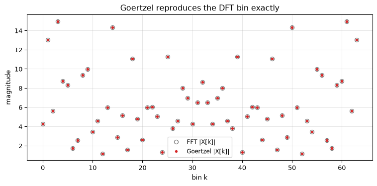
This is not an approximation. For integer \(k\) the recurrence reproduces the DFT bin to floating-point precision. The demo computes every bin of a random signal both ways and reports the largest disagreement.
Show the code
rng = np.random.default_rng(0)N =64x = rng.standard_normal(N)X_fft = np.fft.fft(x)X_goertzel = np.array([goertzel_dft_bin(x, k) for k inrange(N)])max_err = np.max(np.abs(X_goertzel - X_fft))assert max_err <1e-12# matches the caption's "1e-13 level" (measured ~2.8e-13)print(f"largest |Goertzel - FFT| over all {N} bins: {max_err:.2e}")fig, ax = plt.subplots(figsize=(8, 4))ax.plot(np.abs(X_fft), 'o', color='C7', mfc='none', label='FFT |X[k]|')ax.plot(np.abs(X_goertzel), '.', color='C3', label='Goertzel |X[k]|')ax.set_xlabel('bin k'); ax.set_ylabel('magnitude')ax.set_title('Goertzel reproduces the DFT bin exactly')ax.legend(fontsize=9); ax.grid(True, alpha=0.3)fig.tight_layout()plt.show()
largest |Goertzel - FFT| over all 64 bins: 2.80e-13
Figure 1: Goertzel evaluated bin by bin against a full FFT of the same 64-point signal. The two magnitude spectra lie on top of each other; the largest disagreement across all bins is at the 1e-13 level, i.e. floating-point round-off.
Detecting a tone
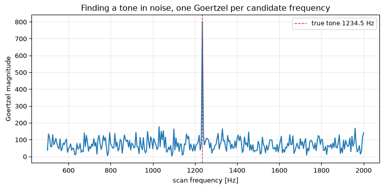
The filter \(H_k\) is a sharp resonator: its pole pair sits on the unit circle at \(\pm\omega_k\), so it responds strongly to energy near that frequency and weakly to everything else. The longer the block \(N\), the narrower the resonance, the finer the frequency discrimination. The demo buries a 1234.5 Hz tone in noise and scans the Goertzel magnitude across a range of frequencies; the response spikes at the tone and is essentially flat elsewhere.
Show the code
fs =8000.0f0 =1234.5n = np.arange(1600) # 0.2 s at 8 kHztone = np.sin(2* np.pi * f0 * n / fs)noisy = tone +2.0* rng.standard_normal(len(n)) # noise power well above the tonescan = np.arange(500, 2001, 5.0)mag = np.array([np.abs(goertzel_freq(noisy, f, fs)) for f in scan])peak_f = scan[np.argmax(mag)]assertabs(peak_f - f0) <=5.0# peak lands on the tone to within the scan stepprint(f"scan peak at {peak_f:.1f} Hz (true tone {f0} Hz)")fig, ax = plt.subplots(figsize=(8, 4))ax.plot(scan, mag, color='C0')ax.axvline(f0, color='C3', linestyle='--', linewidth=1, label=f'true tone {f0} Hz')ax.set_xlabel('scan frequency [Hz]'); ax.set_ylabel('Goertzel magnitude')ax.set_title('Finding a tone in noise, one Goertzel per candidate frequency')ax.legend(fontsize=9); ax.grid(True, alpha=0.3)fig.tight_layout()plt.show()
scan peak at 1235.0 Hz (true tone 1234.5 Hz)
Figure 2: A 1234.5 Hz tone hidden in noise (SNR about -9 dB in this block), recovered by scanning the generalized Goertzel magnitude across frequency. The response peaks sharply at the true tone frequency, marked by the dashed line.
Notice the scan frequencies were not DFT bins: 500, 505, 510 Hz and so on, none of them a multiple of \(f_s/N\). This is the generalized Goertzel. Nothing in the recurrence requires \(\omega\) to be \(2\pi k/N\); any \(\omega = 2\pi f/f_s\) works. You lose the exact-DFT-bin identity but gain the freedom to tune the resonator to the precise frequency you care about, which is exactly what a tone detector wants.
When Goertzel beats the FFT
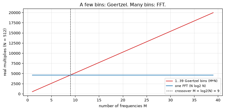
The trade-off is purely about how many frequencies you need. One Goertzel bin costs about \(N\) real multiplies. An FFT costs about \(N\log_2 N\) for all\(N\) bins, so roughly \(\log_2 N\) per bin. Computing \(M\) bins with Goertzel therefore costs \(M N\), and that is cheaper than the FFT when
\[M \lesssim \log_2 N.\]
Show the code
N =512M = np.arange(1, 40)goertzel_ops = M * Nfft_ops = np.full_like(M, int(N * np.log2(N)))crossover = np.log2(N)fig, ax = plt.subplots(figsize=(8, 4))ax.plot(M, goertzel_ops, color='C3', label=f'{M[0]}..{M[-1]} Goertzel bins (M*N)')ax.plot(M, fft_ops, color='C0', label='one FFT (N log2 N)')ax.axvline(crossover, color='k', linestyle='--', linewidth=0.8, label=f'crossover M = log2(N) = {crossover:.0f}')ax.set_xlabel('number of frequencies M'); ax.set_ylabel(f'real multiplies (N = {N})')ax.set_title('A few bins: Goertzel. Many bins: FFT.')ax.legend(fontsize=8); ax.grid(True, alpha=0.3)fig.tight_layout()plt.show()
Figure 3: Multiply count for detecting M frequencies in a length-N block: M independent Goertzel filters (M*N) versus a single FFT (N log2 N). Below the crossover at M = log2(N) bins, Goertzel does less arithmetic; above it, the FFT’s shared structure wins.
The operation count is only half the story, and on a microcontroller often the smaller half. Goertzel also needs no input buffer: it folds each sample in as it arrives and keeps just two state variables per frequency, where an FFT must collect the whole block first and then transform it. It places no constraint on \(N\): you can use 205 samples if that suits your tone spacing, with no zero-padding to the next power of two. And it computes only what you ask for, so eight DTMF tones cost eight filters and not a 256-point transform you mostly discard. Those operational properties are why tone detection on small hardware is a Goertzel job even when the raw multiply count is a near tie.
Four ways to detect a tone
The FFT is not the only alternative worth knowing. ARM’s CMSIS-DSP decodes a DTMF tone three different ways (Yiu 2014, ch. 22), and Goertzel is a natural fourth:
Bandpass FIR tuned to the frequency: linear phase, but many taps, each a multiply-accumulate per sample.
Block FFT, then read the relevant bin: shares work across all frequencies, but computes every bin and must buffer the whole block.
Biquad resonator with a conjugate pole pair just inside the unit circle at the target frequency: only two state variables and a stable narrowband response whose width is set by how close the poles sit to the circle, though the resonant frequency is sensitive to quantisation of the feedback coefficient.
Goertzel: that resonator pushed to the limit, its poles placed exactly on the unit circle so it lands on a DFT bin, read out after \(N\) samples, with a single real coefficient in the recurrence. Poles on the circle are what make it bin-exact, and also marginally stable, the knife-edge this page keeps returning to. For a handful of fixed frequencies it is usually the most economical of the four, which is why it is the standard choice for tone detection on small hardware.
DTMF: the textbook application
Dual-tone multi-frequency signalling (ITU-T Q.23) is the sound a telephone keypad makes. The keys form a four-by-four grid; each key sounds one low-group frequency (its row) plus one high-group frequency (its column).
1209 Hz
1336 Hz
1477 Hz
1633 Hz
697 Hz
1
2
3
A
770 Hz
4
5
6
B
852 Hz
7
8
9
C
941 Hz
*
0
#
D
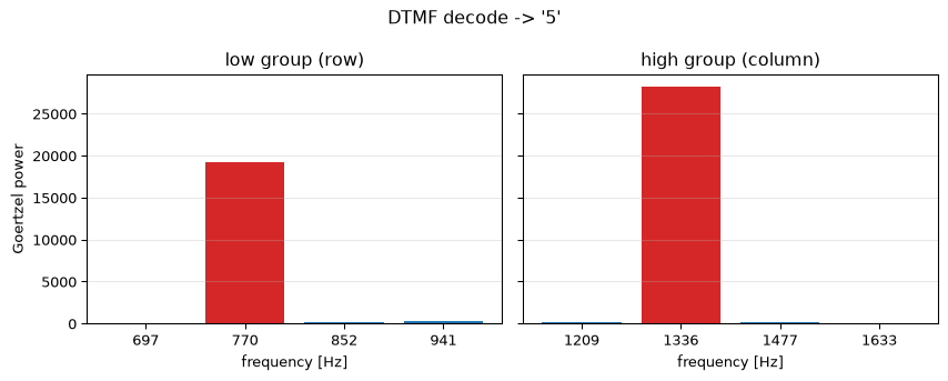
The frequencies were chosen so no one is a harmonic of another, which makes them easy to separate. To decode a block, run eight Goertzel filters, one per frequency, find the strongest in the low group and the strongest in the high group, and read off the key at that row and column. The demo synthesises the tone for key “5” (770 + 1336 Hz), corrupts it with noise, and decodes it from the eight band energies.
Show the code
fs =8000.0key ="5"tone = dtmf_tone(key, fs, 0.04) # 40 ms = 320 samplesnoisy = tone +0.5* rng.standard_normal(len(tone))low_p = [goertzel_power(noisy, 2* np.pi * f / fs) for f in DTMF_LOW]high_p = [goertzel_power(noisy, 2* np.pi * f / fs) for f in DTMF_HIGH]decoded = dtmf_decode(noisy, fs)assert decoded == key # the whole point, checked at renderprint(f"decoded key: {decoded} (row {DTMF_LOW[int(np.argmax(low_p))]:.0f} Hz, "f"col {DTMF_HIGH[int(np.argmax(high_p))]:.0f} Hz)")fig, (axl, axr) = plt.subplots(1, 2, figsize=(9, 3.6), sharey=True)axl.bar([f"{f:.0f}"for f in DTMF_LOW], low_p, color='C0')axl.bar([f"{DTMF_LOW[int(np.argmax(low_p))]:.0f}"], [max(low_p)], color='C3')axl.set_title('low group (row)'); axl.set_ylabel('Goertzel power')axr.bar([f"{f:.0f}"for f in DTMF_HIGH], high_p, color='C0')axr.bar([f"{DTMF_HIGH[int(np.argmax(high_p))]:.0f}"], [max(high_p)], color='C3')axr.set_title('high group (column)')for ax in (axl, axr): ax.set_xlabel('frequency [Hz]'); ax.grid(True, alpha=0.3, axis='y')fig.suptitle(f"DTMF decode -> '{decoded}'")fig.tight_layout()plt.show()
decoded key: 5 (row 770 Hz, col 1336 Hz)
Figure 4: Decoding the DTMF key ‘5’ from a noisy 40 ms block. Eight Goertzel filters measure the energy in the four row frequencies and four column frequencies; the strongest row (770 Hz) and strongest column (1336 Hz) intersect at the key ‘5’.
A real decoder adds a few guards on top of this skeleton: a minimum energy so silence is not decoded, a low-to-high balance check (the two tones should be comparable in level, the “twist” specification), and a second-harmonic test to reject speech that happens to have energy in a band. But the spectral core is exactly the eight filters above. The embedded version is on the hardware page.
Going further
The poles sit on the unit circle, which is a stability knife-edge. A normal filter keeps its poles strictly inside for a stability margin; Goertzel deliberately puts them at \(|z| = 1\). With exact arithmetic that is fine over a finite block, but round-off error in the recurrence has no decay to damp it, so it accumulates roughly linearly in \(N\). For the short blocks tone detection uses this is invisible; for very long blocks, or in narrow fixed-point, the running state can drift and the bin value lose accuracy. How large \(N\) can grow before it matters depends on the word length, and is worth checking rather than assuming.
Block length sets a three-way trade. A longer \(N\) narrows the resonance (better frequency discrimination) and lowers the noise floor, but it also lengthens the latency before a decision and widens the window over which the tone must stay present and steady. DTMF’s choice of a few hundred samples at 8 kHz is a deliberate balance, not a fundamental constant.
There is a sliding form. The block Goertzel here restarts for each window. A sliding Goertzel updates a running bin as each new sample arrives and the oldest leaves, which suits continuous monitoring, at the cost of the marginal-stability bookkeeping above becoming a permanent concern rather than a per-block one.
References
Goertzel’s original note is (Goertzel 1958); the filter-based derivation and the cost comparison with the FFT follow Oppenheim and Schafer (Oppenheim and Schafer 2010, sec. 9.2). The second-order structure the algorithm realises is the one in the DSPIPS workshop notes. The DTMF frequency plan is ITU-T Recommendation Q.23 (ITU-T 1988).
Goertzel, Gerald. 1958. “An Algorithm for the Evaluation of Finite Trigonometric Series.”The American Mathematical Monthly 65 (1): 34–35. https://doi.org/10.2307/2310304.
ITU-T. 1988. “Recommendation Q.23: Technical Features of Push-Button Telephone Sets.” International Telecommunication Union.
Oppenheim, Alan V., and Ronald W. Schafer. 2010. Discrete-Time Signal Processing. 3rd ed. Pearson.
Yiu, Joseph. 2014. The Definitive Guide to ARM Cortex-M3 and Cortex-M4 Processors. 3rd ed. Oxford: Newnes.
Source Code
---title: "The Goertzel Algorithm"subtitle: "One DFT bin from a three-line filter, and why your phone uses it"description-meta: "One DFT bin from a three-line recursive filter: detecting a known tone at a single real multiply per sample, and why telephones use it."---Press a key on a telephone keypad and it plays two tones at once. The far end has to decide, from a short burst of audio, which of sixteen keys you pressed. It does not run a Fourier transform. It runs **Goertzel**: a tiny recursive filter, one per frequency of interest, each costing a single real multiply per audio sample. The whole decoder fits in a few dozen lines of C and runs comfortably on a microcontroller that could never afford a per-sample FFT.That is the situation Goertzel is built for: **you want the spectrum at a few specific frequencies, not the whole thing.** A DFT or FFT computes every bin; if you only care about eight of them, most of that work is thrown away. Goertzel evaluates one bin at a time with a second-order IIR filter, and it does it incrementally, sample by sample, with no input buffer and no power-of-two length requirement.::: {.callout-note title="Prerequisites"}This topic builds on the [DFT and the frequency domain](../../basics/05-frequency-domain.qmd), the [z-domain and poles and zeros](../../basics/04-z-domain.qmd), and the [second-order IIR structures](../../basics/02-discrete-time.qmd) it is built from. The filter here is the same kind of biquad section as in the [biquad chapter](../../basics/09-biquad/index.qmd), tuned for a different job.:::::: {.callout-tip title="Code"}The implementation is [`goertzel.py`](goertzel.py). Save [`test_goertzel.py`](test_goertzel.py) beside it and `pytest test_goertzel.py` runs the checks on it.:::```{python}#| echo: falseimport numpy as npimport matplotlib.pyplot as pltfrom goertzel import (goertzel, goertzel_power, goertzel_dft_bin, goertzel_freq, dtmf_tone, dtmf_decode, DTMF_LOW, DTMF_HIGH, DTMF_KEYS)```<hr>## One bin of the DFTThe $N$-point DFT evaluates, for each bin $k$,$$X[k] = \sum_{n=0}^{N-1} x[n]\, e^{-j 2\pi k n / N}.$$Computing one bin directly is $N$ complex multiply-accumulates. Computing all $N$ bins with an FFT is about $N\log_2 N$. Goertzel sits in between with a trick: it recognises the single sum above as the output, at time $N$, of a **linear filter** driven by $x[n]$.Write $\omega_k = 2\pi k / N$ for the bin frequency. Consider the first-order filter $H(z) = 1 / (1 - e^{j\omega_k} z^{-1})$, a single pole at $z = e^{j\omega_k}$. Feeding $x[n]$ through it and reading the output at $n = N$ gives exactly $X[k]$. That pole is complex, which would mean complex arithmetic on every sample. The Goertzel move is to make the recursive part **real** by multiplying numerator and denominator by $(1 - e^{-j\omega_k}z^{-1})$:$$H_k(z) = \frac{1 - e^{-j\omega_k} z^{-1}}{1 - 2\cos(\omega_k)\, z^{-1} + z^{-2}}.$$The denominator is now real (its two roots are the conjugate pole pair $e^{\pm j\omega_k}$, sitting exactly on the unit circle), and the only coefficient inside the feedback loop is $2\cos(\omega_k)$. This is precisely the second-order IIR section derived in the [DSPIPS workshop notes](../../basics/02-discrete-time.qmd), $H(z) = (1 + b z^{-1})/(1 - a z^{-1} - c z^{-2})$, with $a = 2\cos\omega_k$, $c = -1$, and $b = -e^{-j\omega_k}$.<hr>## The algorithmRealise $H_k(z)$ as a direct-form-II section. The recursive (all-pole) part runs over every input sample,$$s[n] = x[n] + 2\cos(\omega_k)\, s[n-1] - s[n-2], \qquad s[-1] = s[-2] = 0,$$and the feedforward (zero) part is applied **once**, after the last sample, to combine the final two states into the bin value:$$X[k] = e^{j\omega_k}\, s[N-1] - s[N-2].$$That is the entire algorithm. Per sample it is one real multiply ($2\cos\omega_k \cdot s[n-1]$) and two adds. The single complex operation happens once, at the end, not $N$ times.If you only need **how much** energy is at the frequency, not its phase, even that last complex step is unnecessary. The magnitude squared has a real closed form in the final two states:$$|X[k]|^2 = s[N-1]^2 + s[N-2]^2 - 2\cos(\omega_k)\, s[N-1]\, s[N-2].$$No sine, no complex numbers, no square root. A tone detector that compares energy against a threshold runs this and nothing more.### It is the DFT bin, exactlyThis is not an approximation. For integer $k$ the recurrence reproduces the DFT bin to floating-point precision. The demo computes every bin of a random signal both ways and reports the largest disagreement.```{python}#| label: fig-goertzel-vs-fft#| fig-cap: "Goertzel evaluated bin by bin against a full FFT of the same 64-point signal. The two magnitude spectra lie on top of each other; the largest disagreement across all bins is at the 1e-13 level, i.e. floating-point round-off."rng = np.random.default_rng(0)N =64x = rng.standard_normal(N)X_fft = np.fft.fft(x)X_goertzel = np.array([goertzel_dft_bin(x, k) for k inrange(N)])max_err = np.max(np.abs(X_goertzel - X_fft))assert max_err <1e-12# matches the caption's "1e-13 level" (measured ~2.8e-13)print(f"largest |Goertzel - FFT| over all {N} bins: {max_err:.2e}")fig, ax = plt.subplots(figsize=(8, 4))ax.plot(np.abs(X_fft), 'o', color='C7', mfc='none', label='FFT |X[k]|')ax.plot(np.abs(X_goertzel), '.', color='C3', label='Goertzel |X[k]|')ax.set_xlabel('bin k'); ax.set_ylabel('magnitude')ax.set_title('Goertzel reproduces the DFT bin exactly')ax.legend(fontsize=9); ax.grid(True, alpha=0.3)fig.tight_layout()plt.show()```<hr>## Detecting a toneThe filter $H_k$ is a sharp resonator: its pole pair sits on the unit circle at $\pm\omega_k$, so it responds strongly to energy near that frequency and weakly to everything else. The longer the block $N$, the narrower the resonance, the finer the frequency discrimination. The demo buries a 1234.5 Hz tone in noise and scans the Goertzel magnitude across a range of frequencies; the response spikes at the tone and is essentially flat elsewhere.```{python}#| label: fig-tone-detect#| fig-cap: "A 1234.5 Hz tone hidden in noise (SNR about -9 dB in this block), recovered by scanning the generalized Goertzel magnitude across frequency. The response peaks sharply at the true tone frequency, marked by the dashed line."fs =8000.0f0 =1234.5n = np.arange(1600) # 0.2 s at 8 kHztone = np.sin(2* np.pi * f0 * n / fs)noisy = tone +2.0* rng.standard_normal(len(n)) # noise power well above the tonescan = np.arange(500, 2001, 5.0)mag = np.array([np.abs(goertzel_freq(noisy, f, fs)) for f in scan])peak_f = scan[np.argmax(mag)]assertabs(peak_f - f0) <=5.0# peak lands on the tone to within the scan stepprint(f"scan peak at {peak_f:.1f} Hz (true tone {f0} Hz)")fig, ax = plt.subplots(figsize=(8, 4))ax.plot(scan, mag, color='C0')ax.axvline(f0, color='C3', linestyle='--', linewidth=1, label=f'true tone {f0} Hz')ax.set_xlabel('scan frequency [Hz]'); ax.set_ylabel('Goertzel magnitude')ax.set_title('Finding a tone in noise, one Goertzel per candidate frequency')ax.legend(fontsize=9); ax.grid(True, alpha=0.3)fig.tight_layout()plt.show()```Notice the scan frequencies were not DFT bins: 500, 505, 510 Hz and so on, none of them a multiple of $f_s/N$. This is the **generalized Goertzel**. Nothing in the recurrence requires $\omega$ to be $2\pi k/N$; any $\omega = 2\pi f/f_s$ works. You lose the exact-DFT-bin identity but gain the freedom to tune the resonator to the precise frequency you care about, which is exactly what a tone detector wants.<hr>## When Goertzel beats the FFTThe trade-off is purely about how many frequencies you need. One Goertzel bin costs about $N$ real multiplies. An FFT costs about $N\log_2 N$ for **all** $N$ bins, so roughly $\log_2 N$ per bin. Computing $M$ bins with Goertzel therefore costs $M N$, and that is cheaper than the FFT when$$M \lesssim \log_2 N.$$```{python}#| label: fig-crossover#| fig-cap: "Multiply count for detecting M frequencies in a length-N block: M independent Goertzel filters (M*N) versus a single FFT (N log2 N). Below the crossover at M = log2(N) bins, Goertzel does less arithmetic; above it, the FFT's shared structure wins."N =512M = np.arange(1, 40)goertzel_ops = M * Nfft_ops = np.full_like(M, int(N * np.log2(N)))crossover = np.log2(N)fig, ax = plt.subplots(figsize=(8, 4))ax.plot(M, goertzel_ops, color='C3', label=f'{M[0]}..{M[-1]} Goertzel bins (M*N)')ax.plot(M, fft_ops, color='C0', label='one FFT (N log2 N)')ax.axvline(crossover, color='k', linestyle='--', linewidth=0.8, label=f'crossover M = log2(N) = {crossover:.0f}')ax.set_xlabel('number of frequencies M'); ax.set_ylabel(f'real multiplies (N = {N})')ax.set_title('A few bins: Goertzel. Many bins: FFT.')ax.legend(fontsize=8); ax.grid(True, alpha=0.3)fig.tight_layout()plt.show()```The operation count is only half the story, and on a microcontroller often the smaller half. Goertzel also needs **no input buffer**: it folds each sample in as it arrives and keeps just two state variables per frequency, where an FFT must collect the whole block first and then transform it. It places **no constraint on $N$**: you can use 205 samples if that suits your tone spacing, with no zero-padding to the next power of two. And it computes only what you ask for, so eight DTMF tones cost eight filters and not a 256-point transform you mostly discard. Those operational properties are why tone detection on small hardware is a Goertzel job even when the raw multiply count is a near tie.### Four ways to detect a toneThe FFT is not the only alternative worth knowing. ARM's CMSIS-DSP decodes a DTMF tone three different ways [@yiu2014, ch. 22], and Goertzel is a natural fourth:- **Bandpass FIR** tuned to the frequency: linear phase, but many taps, each a multiply-accumulate per sample.- **Block FFT**, then read the relevant bin: shares work across all frequencies, but computes every bin and must buffer the whole block.- **Biquad resonator** with a conjugate pole pair just inside the unit circle at the target frequency: only two state variables and a stable narrowband response whose width is set by how close the poles sit to the circle, though the resonant frequency is sensitive to quantisation of the feedback coefficient.- **Goertzel**: that resonator pushed to the limit, its poles placed exactly *on* the unit circle so it lands on a DFT bin, read out after $N$ samples, with a single real coefficient in the recurrence. Poles on the circle are what make it bin-exact, and also marginally stable, the knife-edge this page keeps returning to. For a handful of fixed frequencies it is usually the most economical of the four, which is why it is the standard choice for tone detection on small hardware.<hr>## DTMF: the textbook applicationDual-tone multi-frequency signalling (ITU-T Q.23) is the sound a telephone keypad makes. The keys form a four-by-four grid; each key sounds one **low-group** frequency (its row) plus one **high-group** frequency (its column).| | 1209 Hz | 1336 Hz | 1477 Hz | 1633 Hz ||---:|:---:|:---:|:---:|:---:|| **697 Hz** | 1 | 2 | 3 | A || **770 Hz** | 4 | 5 | 6 | B || **852 Hz** | 7 | 8 | 9 | C || **941 Hz** | * | 0 | # | D |The frequencies were chosen so no one is a harmonic of another, which makes them easy to separate. To decode a block, run **eight Goertzel filters**, one per frequency, find the strongest in the low group and the strongest in the high group, and read off the key at that row and column. The demo synthesises the tone for key "5" (770 + 1336 Hz), corrupts it with noise, and decodes it from the eight band energies.```{python}#| label: fig-dtmf#| fig-cap: "Decoding the DTMF key '5' from a noisy 40 ms block. Eight Goertzel filters measure the energy in the four row frequencies and four column frequencies; the strongest row (770 Hz) and strongest column (1336 Hz) intersect at the key '5'."fs =8000.0key ="5"tone = dtmf_tone(key, fs, 0.04) # 40 ms = 320 samplesnoisy = tone +0.5* rng.standard_normal(len(tone))low_p = [goertzel_power(noisy, 2* np.pi * f / fs) for f in DTMF_LOW]high_p = [goertzel_power(noisy, 2* np.pi * f / fs) for f in DTMF_HIGH]decoded = dtmf_decode(noisy, fs)assert decoded == key # the whole point, checked at renderprint(f"decoded key: {decoded} (row {DTMF_LOW[int(np.argmax(low_p))]:.0f} Hz, "f"col {DTMF_HIGH[int(np.argmax(high_p))]:.0f} Hz)")fig, (axl, axr) = plt.subplots(1, 2, figsize=(9, 3.6), sharey=True)axl.bar([f"{f:.0f}"for f in DTMF_LOW], low_p, color='C0')axl.bar([f"{DTMF_LOW[int(np.argmax(low_p))]:.0f}"], [max(low_p)], color='C3')axl.set_title('low group (row)'); axl.set_ylabel('Goertzel power')axr.bar([f"{f:.0f}"for f in DTMF_HIGH], high_p, color='C0')axr.bar([f"{DTMF_HIGH[int(np.argmax(high_p))]:.0f}"], [max(high_p)], color='C3')axr.set_title('high group (column)')for ax in (axl, axr): ax.set_xlabel('frequency [Hz]'); ax.grid(True, alpha=0.3, axis='y')fig.suptitle(f"DTMF decode -> '{decoded}'")fig.tight_layout()plt.show()```A real decoder adds a few guards on top of this skeleton: a minimum energy so silence is not decoded, a low-to-high balance check (the two tones should be comparable in level, the "twist" specification), and a second-harmonic test to reject speech that happens to have energy in a band. But the spectral core is exactly the eight filters above. The embedded version is on the [hardware page](embedded.qmd).<hr>## Going further- **The poles sit *on* the unit circle, which is a stability knife-edge.** A normal filter keeps its poles strictly inside for a stability margin; Goertzel deliberately puts them at $|z| = 1$. With exact arithmetic that is fine over a finite block, but round-off error in the recurrence has no decay to damp it, so it accumulates roughly linearly in $N$. For the short blocks tone detection uses this is invisible; for very long blocks, or in narrow fixed-point, the running state can drift and the bin value lose accuracy. How large $N$ can grow before it matters depends on the word length, and is worth checking rather than assuming.- **Block length sets a three-way trade.** A longer $N$ narrows the resonance (better frequency discrimination) and lowers the noise floor, but it also lengthens the latency before a decision and widens the window over which the tone must stay present and steady. DTMF's choice of a few hundred samples at 8 kHz is a deliberate balance, not a fundamental constant.- **There is a sliding form.** The block Goertzel here restarts for each window. A *sliding* Goertzel updates a running bin as each new sample arrives and the oldest leaves, which suits continuous monitoring, at the cost of the marginal-stability bookkeeping above becoming a permanent concern rather than a per-block one.<hr>## ReferencesGoertzel's original note is [@goertzel1958]; the filter-based derivation and the cost comparison with the FFT follow Oppenheim and Schafer [@oppenheim2010discrete, §9.2]. The second-order structure the algorithm realises is the one in the DSPIPS workshop notes. The DTMF frequency plan is ITU-T Recommendation Q.23 [@itu1988q23].::: {#refs}:::