A complete DSP pipeline for heart rate extraction: case study with ESP32 and MAX30102
A photoplethysmograph (PPG) measures blood volume changes by shining light through tissue and measuring the reflected intensity. The raw signal contains the cardiac pulse, respiratory modulation, motion artifacts, and sensor noise — all superimposed. Extracting a reliable heart rate requires a complete DSP pipeline: filtering, detrending, peak/zero-crossing detection, outlier rejection, and rate estimation.
This topic is a case study: it ties together nearly every technique on this site into a single real-world application, using embedded C++ code from an ESP32-based pulse oximeter project. For the complete hardware implementation with FreeRTOS task structure and performance budget, see PPG on Hardware.
Prerequisites
This topic draws on material from across the site. The most relevant pages are:
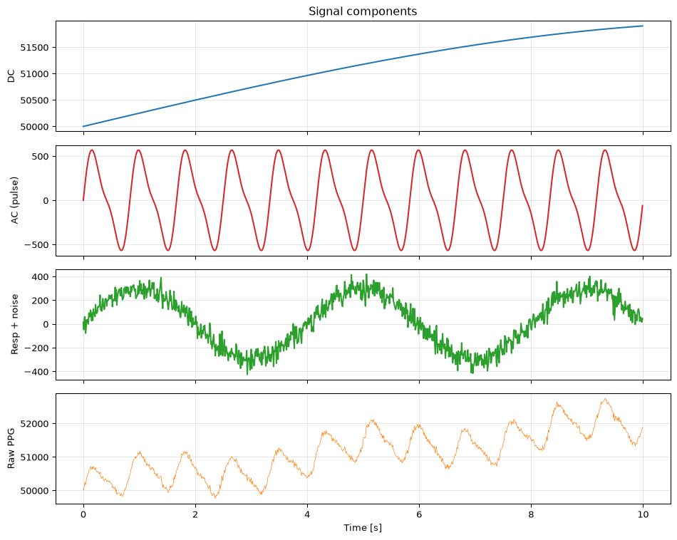
An optical PPG sensor (such as the MAX30102) shines red and infrared LEDs into the skin and measures the reflected light. The measured signal is a superposition of several components:
DC component — light absorbed by tissue, bone, venous blood, and other non-pulsatile structures. This is the dominant part of the signal and varies slowly with sensor placement, skin tone, and ambient light.
AC component — the pulsatile variation caused by arterial blood volume changes during each heartbeat. This is the signal of interest, and it is typically 1–2% of the DC level.
Respiratory modulation — breathing causes periodic changes in venous return and intrathoracic pressure, modulating the PPG baseline at 0.1–0.5 Hz.
Motion artifacts — any movement of the sensor relative to the skin creates large, broadband disturbances that can dwarf the pulse signal.
Sensor noise — quantisation noise, photodetector shot noise, and LED driver noise.
The perfusion index is defined as the ratio of the AC component to the DC component:
Figure 1: A synthetic PPG signal showing the DC baseline, AC pulse, respiratory modulation, and noise.
The processing pipeline
The pipeline architecture mirrors the embedded C++ implementation. Each stage maps directly to a DSP concept covered elsewhere on this site:
Figure 2: The PPG heart-rate pipeline. Each stage maps to a DSP concept covered elsewhere on this site (gray).
Each stage is discussed below with the corresponding C++ implementation and a Python equivalent.
Stage 1: DC removal and AC/DC ratio
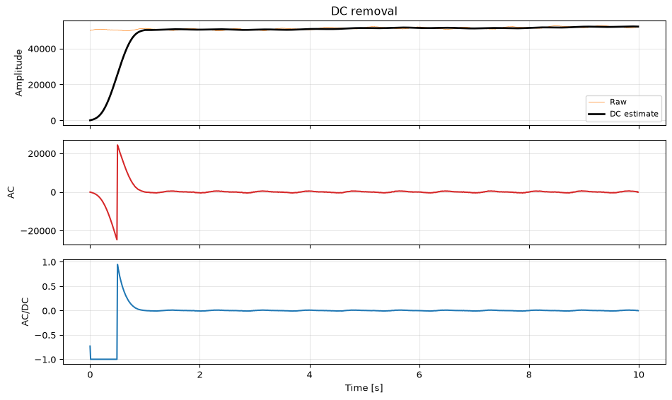
The first step is to separate the slowly varying DC component from the pulsatile AC component. A simple approach: lowpass-filter the raw signal to estimate DC, then subtract the delayed input to get AC:
where \(\Delta\) matches the group delay of the lowpass filter. The AC/DC ratio normalises the pulse amplitude against perfusion level, making the signal comparable across different sensor placements and skin types.
C++ implementation
// DC removal and perfusion index calculation// fe_DC_filter is a lowpass FIR that estimates the DC component// fe_delay compensates for the filter's group delayfloat dc = fe_DC_filter->process(in);float ac = fe_delay->process(in)- dc;float ppg = ac / dc;// perfusion index (normalised pulse)
The delay element fe_delay is critical — without it, the subtraction would compare the current sample against a time-shifted DC estimate, distorting the AC waveform.
Python equivalent
from scipy.signal import firwin, lfilter# Design a lowpass FIR to estimate DC (cutoff well below heart rate)n_taps =101dc_filter = firwin(n_taps, 0.1, fs=fs) # 0.1 Hz cutoffdelay = (n_taps -1) //2# group delay of linear-phase FIR# Estimate DC and extract ACdc_est = lfilter(dc_filter, 1.0, ppg_raw)# Compensate for group delayppg_delayed = np.concatenate([np.zeros(delay), ppg_raw[:len(ppg_raw)-delay]])ac_est = ppg_delayed - dc_est# Avoid division by zero, compute perfusion indexdc_safe = np.where(np.abs(dc_est) >100, dc_est, 100)ppg_normalised = ac_est / dc_safefig, axes = plt.subplots(3, 1, figsize=(10, 6), sharex=True)axes[0].plot(t, ppg_raw, 'C1', linewidth=0.5, label='Raw')axes[0].plot(t, dc_est, 'k', linewidth=2, label='DC estimate')axes[0].legend(fontsize=8)axes[0].set_ylabel('Amplitude')axes[0].set_title('DC removal')axes[1].plot(t, ac_est, 'C3')axes[1].set_ylabel('AC')axes[2].plot(t, ppg_normalised, 'C0')axes[2].set_ylabel('AC/DC')axes[2].set_xlabel('Time [s]')for ax in axes: ax.grid(True, alpha=0.3)fig.tight_layout()plt.show()
Figure 3: DC removal using a lowpass FIR filter. The AC/DC ratio (bottom) isolates the pulse independent of absolute signal level.
Stage 2: Bandpass filtering
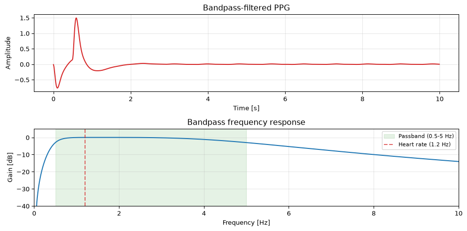
A biquad cascade (second-order sections) bandpass-filters the normalised signal to isolate the heart rate band: 0.5–5 Hz (30–300 BPM). This rejects both the respiratory modulation below 0.5 Hz and high-frequency noise above 5 Hz.
C++ implementation — transposed direct form II biquad
The biquad uses transposed direct form II, which is preferred for floating-point implementations because zeros are processed first, preventing the explosion of internal states that can occur in direct form I:
// Transposed direct form II biquad — one second-order section// Preferred since zeros are implemented first, reducing// explosion of internal statesfloat Biquad::process(float in){float out = b[0]* in + w[0]; w[0]= w[1]+ b[1]* in - a[1]* out; w[1]= b[2]* in - a[2]* out;return out;}
The cascade chains two of these sections for a 4th-order bandpass. An important implementation detail is the init() function that preloads the state variables with the DC value of the first sample, avoiding the startup transient that would otherwise produce a large spike and trigger a false first beat:
void Biquad::init(float dc_value){// Pre-fill states to avoid startup transient// Solve for steady-state: w[n] when input = output = dc_value w[1]= dc_value *(b[2]- a[2]* b[0]); w[0]= dc_value *(b[1]- a[1]* b[0])+ w[1];}
Figure 4: Bandpass filtering isolates the heart rate band (0.5-5 Hz). The frequency response shows the passband aligned with the cardiac frequency range.
Stage 3: Beat detection
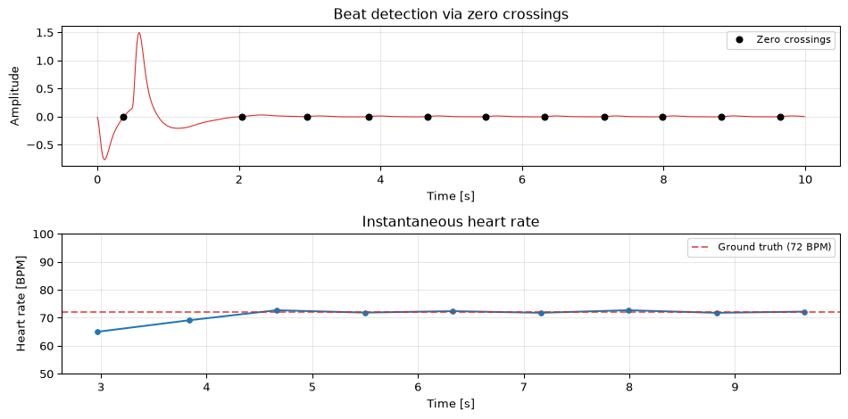
The beat detector finds cardiac pulses by looking for rising zero crossings in the bandpass-filtered signal. Each rising zero crossing corresponds to the onset of one heartbeat cycle. The inter-beat interval (IBI) is converted to beats per minute:
A range check rejects physiologically impossible beats: anything outside 40–120 BPM (IBI of 500–1500 ms) is discarded.
C++ implementation
// Zero-crossing beat detectorbool PulseDetector::process(float sample){bool beat =false;if(prev_sample <0.0f&& sample >=0.0f){// Rising zero crossing detecteduint32_t now = millis();uint32_t ibi = now - last_beat_time;if(ibi >500&& ibi <1500){// 40-120 BPM range heart_rate =60000.0f/ ibi; beat =true;} last_beat_time = now;} prev_sample = sample;return beat;}
Python equivalent
# Detect rising zero crossingszero_crossings = []for i inrange(1, len(ppg_filtered)):if ppg_filtered[i-1] <0and ppg_filtered[i] >=0:# Linear interpolation for sub-sample accuracy frac =-ppg_filtered[i-1] / (ppg_filtered[i] - ppg_filtered[i-1]) zero_crossings.append(i -1+ frac)zero_crossings = np.array(zero_crossings)# Calculate IBIs and heart ratesibis = np.diff(zero_crossings) / fs # in secondshr_raw =60.0/ ibis # in BPM# Range check: 40-120 BPMvalid = (hr_raw >=40) & (hr_raw <=120)hr_valid = hr_raw[valid]t_hr = zero_crossings[1:][valid] / fsfig, axes = plt.subplots(2, 1, figsize=(10, 5))axes[0].plot(t, ppg_filtered, 'C3', linewidth=0.8)zc_idx = zero_crossings.astype(int)zc_idx = zc_idx[zc_idx <len(t)]axes[0].plot(t[zc_idx], np.zeros(len(zc_idx)), 'ko', markersize=5, label='Zero crossings')axes[0].set_xlabel('Time [s]')axes[0].set_ylabel('Amplitude')axes[0].set_title('Beat detection via zero crossings')axes[0].legend(fontsize=8)axes[0].grid(True, alpha=0.3)axes[1].plot(t_hr, hr_valid, 'C0o-', markersize=4)axes[1].axhline(72, color='C3', linestyle='--', alpha=0.7, label='Ground truth (72 BPM)')axes[1].set_xlabel('Time [s]')axes[1].set_ylabel('Heart rate [BPM]')axes[1].set_title('Instantaneous heart rate')axes[1].legend(fontsize=8)axes[1].grid(True, alpha=0.3)axes[1].set_ylim(50, 100)fig.tight_layout()plt.show()
Figure 5: Rising zero crossings in the filtered PPG mark the start of each heartbeat. The detected heart rate matches the 72 BPM ground truth.
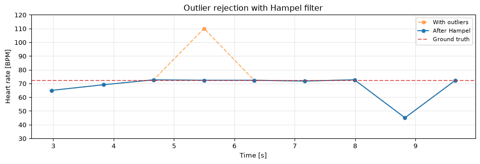
Stage 4: Outlier rejection
Even with bandpass filtering and range checks, the raw heart rate sequence can contain outliers — a motion artifact that sneaks through, or an irregular beat that gives an abnormal IBI. The Hampel filter rejects these by comparing each estimate against a sliding-window median:
Compute the median of the last \(k\) heart rate values
Compute the MAD (median absolute deviation) of the window
If the current value deviates from the median by more than \(n_\sigma \times \text{MAD}\), replace it with the median
This is exactly the robust outlier detection approach covered in the outlier detection topic, applied to a 1D time series of rate estimates rather than a spatial signal.
C++ implementation
// Hampel filter for heart rate outlier rejectionfloat HampelFilter::process(float hr){ buffer[idx]= hr; idx =(idx +1)% window_size;// Sort a copy to find medianstd::copy(buffer, buffer + window_size, sorted);std::sort(sorted, sorted + window_size);float median = sorted[window_size /2];// Compute MADfor(int i =0; i < window_size; i++) deviations[i]=std::abs(buffer[i]- median);std::sort(deviations, deviations + window_size);float mad =1.4826f* deviations[window_size /2];// scale to σ// Reject if too far from medianif(std::abs(hr - median)> n_sigma * mad)return median;return hr;}
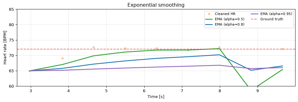
Figure 7: Exponential smoothing with different alpha values. Higher alpha gives smoother but laggier output.
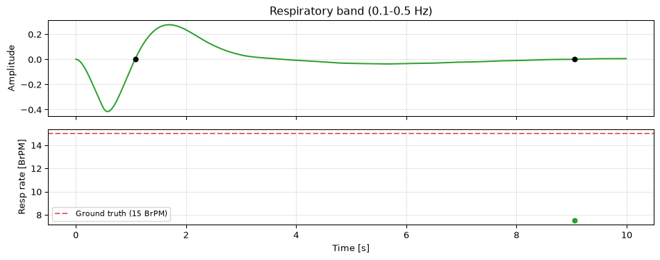
Respiratory rate from PPG
The same pipeline architecture can extract respiratory rate. Breathing modulates the PPG signal at 0.1–0.5 Hz (6–30 breaths per minute) through changes in venous return and intrathoracic pressure.
The respiratory pipeline reuses the same components with different parameters:
Parameter
Heart rate
Respiratory rate
Bandpass
0.5 – 5 Hz
0.1 – 0.5 Hz
BPM range
40 – 120
6 – 30
Detector
pulse_detector
resp_detector
In the C++ implementation, the respiratory detector is a second instance of the same ZeroCrossingDetector class, fed by a different biquad cascade tuned to the respiratory band:
// Same pipeline, different frequency bandfloat resp_filtered = resp_biquad_cascade->process(ppg);bool breath = resp_detector->process(resp_filtered);if(breath){ resp_rate =60000.0f/ resp_ibi;// breaths per minute}
Figure 8: Respiratory rate extraction uses the same pipeline architecture with a lower bandpass (0.1-0.5 Hz).
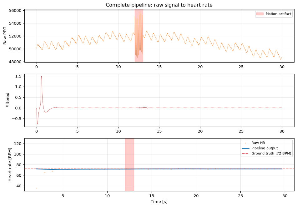
Full pipeline demonstration
Putting it all together: generate a synthetic PPG with known heart rate, process it through the complete pipeline, and compare the output against ground truth.
Figure 9: Complete pipeline from raw PPG to smoothed heart rate estimate. The pipeline converges to the true 72 BPM within a few beats.
Hardware
The embedded implementation runs on an ESP32 microcontroller with the following peripherals:
Component
Role
Interface
MAX30102
PPG sensor (red + IR LEDs, photodetector)
I2C
LSM303C
3-axis accelerometer (motion detection)
I2C
PCM5102
Audio DAC (sonification / feedback)
I2S
The MAX30102 samples at 100 Hz with 18-bit ADC resolution. Both red and infrared channels are read, though only the IR channel is used for heart rate — the red channel is reserved for future SpO2 estimation.
The entire DSP pipeline (DC removal, biquad cascade, zero-crossing detection, Hampel filter, EMA) runs in the main loop at 100 Hz with negligible CPU load. The ESP32’s 240 MHz dual-core processor is vastly overpowered for this task, but it also handles WiFi, BLE, and the display update.
Open questions
Motion artifact removal. The LSM303C accelerometer provides a reference signal for adaptive noise cancellation (see adaptive filtering). The idea: use the accelerometer signal as the reference input to an LMS or NLMS filter, and subtract the estimated motion component from the PPG. This is the classic adaptive noise cancellation architecture, but the nonlinear coupling between motion and optical signal makes it challenging in practice.
SpO2 estimation. Blood oxygen saturation can be estimated from the ratio of AC/DC values at two wavelengths (red and infrared). The MAX30102 provides both channels. The relationship between the ratio-of-ratios \(R = (\text{AC}_\text{red}/\text{DC}_\text{red}) / (\text{AC}_\text{IR}/\text{DC}_\text{IR})\) and SpO2 is approximately linear in the 70–100% range but requires empirical calibration.
Wearable vs. fingertip placement. Fingertip PPG gives strong signals (high perfusion) but is impractical for continuous monitoring. Wrist-worn sensors have much lower perfusion and more motion artifacts. The pipeline would need more aggressive filtering and possibly multi-wavelength approaches.
Deep learning approaches. End-to-end neural networks (1D CNNs, transformers) trained on large PPG datasets can outperform the traditional pipeline, especially under motion. But they are opaque, require large training sets, and do not run easily on microcontrollers — the interpretability and efficiency of the classical pipeline remain advantages.
Source Code
---title: "PPG Signal Processing"subtitle: "A complete DSP pipeline for heart rate extraction: case study with ESP32 and MAX30102"---A photoplethysmograph (PPG) measures blood volume changes by shining light through tissue and measuring the reflected intensity. The raw signal contains the cardiac pulse, respiratory modulation, motion artifacts, and sensor noise --- all superimposed. Extracting a reliable heart rate requires a complete DSP pipeline: filtering, detrending, peak/zero-crossing detection, outlier rejection, and rate estimation.This topic is a **case study**: it ties together nearly every technique on this site into a single real-world application, using embedded C++ code from an ESP32-based pulse oximeter project. For the complete hardware implementation with FreeRTOS task structure and performance budget, see [PPG on Hardware](embedded.qmd).::: {.callout-note title="Prerequisites"}This topic draws on material from across the site. The most relevant pages are:- [Biquad filters](../biquad/index.qmd) (+ [embedded page](../biquad/embedded.qmd)) --- the core filtering building block- [Zero-crossing detection](../zero-crossing/index.qmd) --- beat detection- [Outlier detection](../outlier-detection/index.qmd) --- Hampel filter for rate cleaning- [Filter design (Ch6)](../../basics/06-filter-design.qmd) --- IIR/FIR design principles- [Noise and SNR (Ch3)](../../basics/03-noise-snr.qmd) --- signal quality- [Adaptive filtering](../adaptive-filtering/index.qmd) --- for motion artifact removal (future work):::---## The PPG signalAn optical PPG sensor (such as the MAX30102) shines red and infrared LEDs into the skin and measures the reflected light. The measured signal is a superposition of several components:- **DC component** --- light absorbed by tissue, bone, venous blood, and other non-pulsatile structures. This is the dominant part of the signal and varies slowly with sensor placement, skin tone, and ambient light.- **AC component** --- the pulsatile variation caused by arterial blood volume changes during each heartbeat. This is the signal of interest, and it is typically 1--2% of the DC level.- **Respiratory modulation** --- breathing causes periodic changes in venous return and intrathoracic pressure, modulating the PPG baseline at 0.1--0.5 Hz.- **Motion artifacts** --- any movement of the sensor relative to the skin creates large, broadband disturbances that can dwarf the pulse signal.- **Sensor noise** --- quantisation noise, photodetector shot noise, and LED driver noise.The **perfusion index** is defined as the ratio of the AC component to the DC component:$$\text{PI} = \frac{\text{AC}}{\text{DC}} \times 100\%$$A healthy finger-tip reading gives PI around 1--5%. Lower perfusion (cold hands, poor contact) means a weaker signal and harder extraction.```{python}#| label: fig-ppg-components#| fig-cap: "A synthetic PPG signal showing the DC baseline, AC pulse, respiratory modulation, and noise."import numpy as npimport matplotlib.pyplot as pltrng = np.random.default_rng(42)fs =100# Hz (typical MAX30102 sample rate)t = np.arange(0, 10, 1/fs)# DC component (slowly varying baseline)dc =50000+2000* np.sin(2* np.pi *0.02* t)# AC component (cardiac pulse, ~1.2 Hz = 72 BPM)hr_freq =1.2# Realistic pulse shape: sharper systolic peakphase =2* np.pi * hr_freq * tac =500* (np.sin(phase) +0.3* np.sin(2* phase))# Respiratory modulation (~0.25 Hz = 15 breaths/min)resp =300* np.sin(2* np.pi *0.25* t)# Sensor noisenoise = rng.standard_normal(len(t)) *50# Combined signalppg_raw = dc + ac + resp + noisefig, axes = plt.subplots(4, 1, figsize=(10, 8), sharex=True)axes[0].plot(t, dc, 'C0')axes[0].set_ylabel('DC')axes[0].set_title('Signal components')axes[1].plot(t, ac, 'C3')axes[1].set_ylabel('AC (pulse)')axes[2].plot(t, resp + noise, 'C2')axes[2].set_ylabel('Resp + noise')axes[3].plot(t, ppg_raw, 'C1', linewidth=0.5)axes[3].set_ylabel('Raw PPG')axes[3].set_xlabel('Time [s]')for ax in axes: ax.grid(True, alpha=0.3)fig.tight_layout()plt.show()```---## The processing pipelineThe pipeline architecture mirrors the embedded C++ implementation. Each stage maps directly to a DSP concept covered elsewhere on this site:```{dot}//| label: fig-ppg-pipeline//| echo: false//| fig-cap: "The PPG heart-rate pipeline. Each stage maps to a DSP concept covered elsewhere on this site (gray)."digraph { rankdir=TB graph [pad=0.15 ranksep=0.28 nodesep=0.3] node [fontname="sans-serif" fontsize=12 shape=box height=0.4 margin="0.12,0.05"] edge [arrowsize=0.7] s0 [label="MAX30102 (I2C, 100 Hz)"] s1 [label="DC removal (FIR highpass)"] s2 [label="AC / DC ratio (perfusion index)"] s3 [label="Bandpass filter (biquad cascade)"] s4 [label="Zero-crossing detector"] s5 [label="IBI → heart rate (BPM)"] s6 [label="Hampel outlier filter"] s7 [label="Exponential smoothing"] s8 [label="Heart rate estimate" style=filled fillcolor="#eef3f8"] s0->s1->s2->s3->s4->s5->s6->s7->s8 n1 [label="detrending, filter design" shape=plaintext fontcolor="#888" fontsize=10] n2 [label="normalisation" shape=plaintext fontcolor="#888" fontsize=10] n3 [label="biquad filters, IIR design" shape=plaintext fontcolor="#888" fontsize=10] n4 [label="zero-crossing detection" shape=plaintext fontcolor="#888" fontsize=10] n5 [label="rate estimation" shape=plaintext fontcolor="#888" fontsize=10] n6 [label="outlier detection" shape=plaintext fontcolor="#888" fontsize=10] n7 [label="smoothing" shape=plaintext fontcolor="#888" fontsize=10] s1->n1 [style=dotted dir=none color="#bbb" constraint=false] s2->n2 [style=dotted dir=none color="#bbb" constraint=false] s3->n3 [style=dotted dir=none color="#bbb" constraint=false] s4->n4 [style=dotted dir=none color="#bbb" constraint=false] s5->n5 [style=dotted dir=none color="#bbb" constraint=false] s6->n6 [style=dotted dir=none color="#bbb" constraint=false] s7->n7 [style=dotted dir=none color="#bbb" constraint=false] {rank=same; s1 n1} {rank=same; s2 n2} {rank=same; s3 n3} {rank=same; s4 n4} {rank=same; s5 n5} {rank=same; s6 n6} {rank=same; s7 n7}}```Each stage is discussed below with the corresponding C++ implementation and a Python equivalent.---## Stage 1: DC removal and AC/DC ratioThe first step is to separate the slowly varying DC component from the pulsatile AC component. A simple approach: lowpass-filter the raw signal to estimate DC, then subtract the delayed input to get AC:$$\text{dc}[n] = \text{LPF}\{x[n]\}$$$$\text{ac}[n] = x[n - \Delta] - \text{dc}[n]$$where $\Delta$ matches the group delay of the lowpass filter. The AC/DC ratio normalises the pulse amplitude against perfusion level, making the signal comparable across different sensor placements and skin types.### C++ implementation```cpp// DC removal and perfusion index calculation// fe_DC_filter is a lowpass FIR that estimates the DC component// fe_delay compensates for the filter's group delayfloat dc = fe_DC_filter->process(in);float ac = fe_delay->process(in)- dc;float ppg = ac / dc;// perfusion index (normalised pulse)```The delay element `fe_delay` is critical --- without it, the subtraction would compare the current sample against a time-shifted DC estimate, distorting the AC waveform.### Python equivalent```{python}#| label: fig-dc-removal#| fig-cap: "DC removal using a lowpass FIR filter. The AC/DC ratio (bottom) isolates the pulse independent of absolute signal level."from scipy.signal import firwin, lfilter# Design a lowpass FIR to estimate DC (cutoff well below heart rate)n_taps =101dc_filter = firwin(n_taps, 0.1, fs=fs) # 0.1 Hz cutoffdelay = (n_taps -1) //2# group delay of linear-phase FIR# Estimate DC and extract ACdc_est = lfilter(dc_filter, 1.0, ppg_raw)# Compensate for group delayppg_delayed = np.concatenate([np.zeros(delay), ppg_raw[:len(ppg_raw)-delay]])ac_est = ppg_delayed - dc_est# Avoid division by zero, compute perfusion indexdc_safe = np.where(np.abs(dc_est) >100, dc_est, 100)ppg_normalised = ac_est / dc_safefig, axes = plt.subplots(3, 1, figsize=(10, 6), sharex=True)axes[0].plot(t, ppg_raw, 'C1', linewidth=0.5, label='Raw')axes[0].plot(t, dc_est, 'k', linewidth=2, label='DC estimate')axes[0].legend(fontsize=8)axes[0].set_ylabel('Amplitude')axes[0].set_title('DC removal')axes[1].plot(t, ac_est, 'C3')axes[1].set_ylabel('AC')axes[2].plot(t, ppg_normalised, 'C0')axes[2].set_ylabel('AC/DC')axes[2].set_xlabel('Time [s]')for ax in axes: ax.grid(True, alpha=0.3)fig.tight_layout()plt.show()```---## Stage 2: Bandpass filteringA biquad cascade (second-order sections) bandpass-filters the normalised signal to isolate the heart rate band: **0.5--5 Hz** (30--300 BPM). This rejects both the respiratory modulation below 0.5 Hz and high-frequency noise above 5 Hz.### C++ implementation --- transposed direct form II biquadThe biquad uses **transposed direct form II**, which is preferred for floating-point implementations because zeros are processed first, preventing the explosion of internal states that can occur in direct form I:```cpp// Transposed direct form II biquad — one second-order section// Preferred since zeros are implemented first, reducing// explosion of internal statesfloat Biquad::process(float in){float out = b[0]* in + w[0]; w[0]= w[1]+ b[1]* in - a[1]* out; w[1]= b[2]* in - a[2]* out;return out;}```The cascade chains two of these sections for a 4th-order bandpass. An important implementation detail is the `init()` function that preloads the state variables with the DC value of the first sample, avoiding the startup transient that would otherwise produce a large spike and trigger a false first beat:```cppvoid Biquad::init(float dc_value){// Pre-fill states to avoid startup transient// Solve for steady-state: w[n] when input = output = dc_value w[1]= dc_value *(b[2]- a[2]* b[0]); w[0]= dc_value *(b[1]- a[1]* b[0])+ w[1];}```### Python equivalent```{python}#| label: fig-bandpass#| fig-cap: "Bandpass filtering isolates the heart rate band (0.5-5 Hz). The frequency response shows the passband aligned with the cardiac frequency range."from scipy.signal import butter, sosfilt, sosfreqz# 4th-order Butterworth bandpass: 0.5 - 5 Hzsos = butter(2, [0.5, 5.0], btype='band', fs=fs, output='sos')# Apply bandpass to normalised PPGppg_filtered = sosfilt(sos, ppg_normalised)fig, axes = plt.subplots(2, 1, figsize=(10, 5))# Time domainaxes[0].plot(t, ppg_filtered, 'C3')axes[0].set_xlabel('Time [s]')axes[0].set_ylabel('Amplitude')axes[0].set_title('Bandpass-filtered PPG')axes[0].grid(True, alpha=0.3)# Frequency responsew, H = sosfreqz(sos, worN=2048, fs=fs)axes[1].plot(w, 20* np.log10(np.abs(H) +1e-12), 'C0')axes[1].axvspan(0.5, 5.0, alpha=0.1, color='green', label='Passband (0.5-5 Hz)')axes[1].axvline(hr_freq, color='C3', linestyle='--', alpha=0.7, label=f'Heart rate ({hr_freq} Hz)')axes[1].set_xlabel('Frequency [Hz]')axes[1].set_ylabel('Gain [dB]')axes[1].set_title('Bandpass frequency response')axes[1].set_xlim(0, 10)axes[1].set_ylim(-40, 5)axes[1].legend(fontsize=8)axes[1].grid(True, alpha=0.3)fig.tight_layout()plt.show()```---## Stage 3: Beat detectionThe beat detector finds cardiac pulses by looking for **rising zero crossings** in the bandpass-filtered signal. Each rising zero crossing corresponds to the onset of one heartbeat cycle. The inter-beat interval (IBI) is converted to beats per minute:$$\text{HR} = \frac{60000}{\text{IBI}_\text{ms}}$$A range check rejects physiologically impossible beats: anything outside 40--120 BPM (IBI of 500--1500 ms) is discarded.### C++ implementation```cpp// Zero-crossing beat detectorbool PulseDetector::process(float sample){bool beat =false;if(prev_sample <0.0f&& sample >=0.0f){// Rising zero crossing detecteduint32_t now = millis();uint32_t ibi = now - last_beat_time;if(ibi >500&& ibi <1500){// 40-120 BPM range heart_rate =60000.0f/ ibi; beat =true;} last_beat_time = now;} prev_sample = sample;return beat;}```### Python equivalent```{python}#| label: fig-beat-detection#| fig-cap: "Rising zero crossings in the filtered PPG mark the start of each heartbeat. The detected heart rate matches the 72 BPM ground truth."# Detect rising zero crossingszero_crossings = []for i inrange(1, len(ppg_filtered)):if ppg_filtered[i-1] <0and ppg_filtered[i] >=0:# Linear interpolation for sub-sample accuracy frac =-ppg_filtered[i-1] / (ppg_filtered[i] - ppg_filtered[i-1]) zero_crossings.append(i -1+ frac)zero_crossings = np.array(zero_crossings)# Calculate IBIs and heart ratesibis = np.diff(zero_crossings) / fs # in secondshr_raw =60.0/ ibis # in BPM# Range check: 40-120 BPMvalid = (hr_raw >=40) & (hr_raw <=120)hr_valid = hr_raw[valid]t_hr = zero_crossings[1:][valid] / fsfig, axes = plt.subplots(2, 1, figsize=(10, 5))axes[0].plot(t, ppg_filtered, 'C3', linewidth=0.8)zc_idx = zero_crossings.astype(int)zc_idx = zc_idx[zc_idx <len(t)]axes[0].plot(t[zc_idx], np.zeros(len(zc_idx)), 'ko', markersize=5, label='Zero crossings')axes[0].set_xlabel('Time [s]')axes[0].set_ylabel('Amplitude')axes[0].set_title('Beat detection via zero crossings')axes[0].legend(fontsize=8)axes[0].grid(True, alpha=0.3)axes[1].plot(t_hr, hr_valid, 'C0o-', markersize=4)axes[1].axhline(72, color='C3', linestyle='--', alpha=0.7, label='Ground truth (72 BPM)')axes[1].set_xlabel('Time [s]')axes[1].set_ylabel('Heart rate [BPM]')axes[1].set_title('Instantaneous heart rate')axes[1].legend(fontsize=8)axes[1].grid(True, alpha=0.3)axes[1].set_ylim(50, 100)fig.tight_layout()plt.show()```---## Stage 4: Outlier rejectionEven with bandpass filtering and range checks, the raw heart rate sequence can contain outliers --- a motion artifact that sneaks through, or an irregular beat that gives an abnormal IBI. The **Hampel filter** rejects these by comparing each estimate against a sliding-window median:1. Compute the median of the last $k$ heart rate values2. Compute the MAD (median absolute deviation) of the window3. If the current value deviates from the median by more than $n_\sigma \times \text{MAD}$, replace it with the medianThis is exactly the robust outlier detection approach covered in the [outlier detection topic](../outlier-detection/index.qmd), applied to a 1D time series of rate estimates rather than a spatial signal.### C++ implementation```cpp// Hampel filter for heart rate outlier rejectionfloat HampelFilter::process(float hr){ buffer[idx]= hr; idx =(idx +1)% window_size;// Sort a copy to find medianstd::copy(buffer, buffer + window_size, sorted);std::sort(sorted, sorted + window_size);float median = sorted[window_size /2];// Compute MADfor(int i =0; i < window_size; i++) deviations[i]=std::abs(buffer[i]- median);std::sort(deviations, deviations + window_size);float mad =1.4826f* deviations[window_size /2];// scale to σ// Reject if too far from medianif(std::abs(hr - median)> n_sigma * mad)return median;return hr;}```### Python equivalent```{python}#| label: fig-hampel#| fig-cap: "The Hampel filter replaces outlier heart rate estimates with the local median. Here the clean signal passes through unchanged."def hampel_filter(data, window_size=5, n_sigma=3.0):"""Hampel filter: replace outliers with local median.""" result = data.copy() half_w = window_size //2for i inrange(half_w, len(data) - half_w): window = data[i - half_w:i + half_w +1] median = np.median(window) mad =1.4826* np.median(np.abs(window - median))if mad >0and np.abs(data[i] - median) > n_sigma * mad: result[i] = medianreturn result# Add some artificial outliers for demonstrationhr_with_outliers = hr_valid.copy()iflen(hr_with_outliers) >5: hr_with_outliers[3] =110# inject outlier hr_with_outliers[7] =45# inject outlierhr_cleaned = hampel_filter(hr_with_outliers, window_size=5, n_sigma=2.0)fig, ax = plt.subplots(figsize=(10, 3.5))ax.plot(t_hr, hr_with_outliers, 'C1o--', markersize=5, alpha=0.6, label='With outliers')ax.plot(t_hr, hr_cleaned, 'C0o-', markersize=5, label='After Hampel')ax.axhline(72, color='C3', linestyle='--', alpha=0.7, label='Ground truth')ax.set_xlabel('Time [s]')ax.set_ylabel('Heart rate [BPM]')ax.set_title('Outlier rejection with Hampel filter')ax.legend(fontsize=8)ax.grid(True, alpha=0.3)ax.set_ylim(30, 120)fig.tight_layout()plt.show()```---## Stage 5: Rate smoothingThe final stage applies an **exponential moving average** (EMA) to produce a smooth, displayable heart rate:$$\bar{h}[n] = \alpha \cdot \bar{h}[n-1] + (1 - \alpha) \cdot h[n]$$The smoothing factor $\alpha$ controls the trade-off:- High $\alpha$ (e.g., 0.95): smooth output, slow to respond to real changes- Low $\alpha$ (e.g., 0.5): responsive but noisyIn the embedded system, $\alpha = 0.9$ provides a good balance for a resting heart rate display.### C++ implementation```cpp// Exponential moving average for heart rate smoothingfloat EMA::process(float hr){if(!initialised){ avg = hr; initialised =true;}else{ avg = alpha * avg +(1.0f- alpha)* hr;}return avg;}```### Python equivalent```{python}#| label: fig-smoothing#| fig-cap: "Exponential smoothing with different alpha values. Higher alpha gives smoother but laggier output."def ema_filter(data, alpha):"""Exponential moving average.""" result = np.zeros_like(data) result[0] = data[0]for i inrange(1, len(data)): result[i] = alpha * result[i-1] + (1- alpha) * data[i]return resultfig, ax = plt.subplots(figsize=(10, 3.5))ax.plot(t_hr, hr_cleaned, 'C1o', markersize=4, alpha=0.4, label='Cleaned HR')for alpha, color in [(0.5, 'C2'), (0.8, 'C0'), (0.95, 'C4')]: smoothed = ema_filter(hr_cleaned, alpha) ax.plot(t_hr, smoothed, color, linewidth=2, label=f'EMA (alpha={alpha})')ax.axhline(72, color='C3', linestyle='--', alpha=0.7, label='Ground truth')ax.set_xlabel('Time [s]')ax.set_ylabel('Heart rate [BPM]')ax.set_title('Exponential smoothing')ax.legend(fontsize=8, ncol=2)ax.grid(True, alpha=0.3)ax.set_ylim(60, 85)fig.tight_layout()plt.show()```---## Respiratory rate from PPGThe same pipeline architecture can extract respiratory rate. Breathing modulates the PPG signal at 0.1--0.5 Hz (6--30 breaths per minute) through changes in venous return and intrathoracic pressure.The respiratory pipeline reuses the same components with different parameters:| Parameter | Heart rate | Respiratory rate ||---|---|---|| Bandpass | 0.5 -- 5 Hz | 0.1 -- 0.5 Hz || BPM range | 40 -- 120 | 6 -- 30 || Detector | `pulse_detector` | `resp_detector` |In the C++ implementation, the respiratory detector is a second instance of the same `ZeroCrossingDetector` class, fed by a different biquad cascade tuned to the respiratory band:```cpp// Same pipeline, different frequency bandfloat resp_filtered = resp_biquad_cascade->process(ppg);bool breath = resp_detector->process(resp_filtered);if(breath){ resp_rate =60000.0f/ resp_ibi;// breaths per minute}``````{python}#| label: fig-respiratory#| fig-cap: "Respiratory rate extraction uses the same pipeline architecture with a lower bandpass (0.1-0.5 Hz)."# Bandpass for respiratory bandsos_resp = butter(2, [0.1, 0.5], btype='band', fs=fs, output='sos')ppg_resp = sosfilt(sos_resp, ppg_normalised)# Detect breathing cycles (zero crossings)resp_zc = []for i inrange(1, len(ppg_resp)):if ppg_resp[i-1] <0and ppg_resp[i] >=0: resp_zc.append(i)resp_zc = np.array(resp_zc)iflen(resp_zc) >1: resp_ibis = np.diff(resp_zc) / fs resp_rates =60.0/ resp_ibis valid_resp = (resp_rates >=6) & (resp_rates <=30)fig, axes = plt.subplots(2, 1, figsize=(10, 4), sharex=True)axes[0].plot(t, ppg_resp, 'C2')iflen(resp_zc) >0: zc_valid = resp_zc[resp_zc <len(t)] axes[0].plot(t[zc_valid], np.zeros(len(zc_valid)), 'ko', markersize=5)axes[0].set_ylabel('Amplitude')axes[0].set_title('Respiratory band (0.1-0.5 Hz)')axes[0].grid(True, alpha=0.3)iflen(resp_zc) >1: t_resp = resp_zc[1:] / fs axes[1].plot(t_resp[valid_resp], resp_rates[valid_resp], 'C2o-', markersize=5) axes[1].axhline(15, color='C3', linestyle='--', alpha=0.7, label='Ground truth (15 BrPM)') axes[1].set_ylabel('Resp rate [BrPM]') axes[1].legend(fontsize=8)axes[1].set_xlabel('Time [s]')axes[1].grid(True, alpha=0.3)fig.tight_layout()plt.show()```---## Full pipeline demonstrationPutting it all together: generate a synthetic PPG with known heart rate, process it through the complete pipeline, and compare the output against ground truth.```{python}#| label: fig-full-pipeline#| fig-cap: "Complete pipeline from raw PPG to smoothed heart rate estimate. The pipeline converges to the true 72 BPM within a few beats."# Generate a longer synthetic PPG (30 seconds)t_long = np.arange(0, 30, 1/fs)dc_long =50000+2000* np.sin(2* np.pi *0.02* t_long)phase_long =2* np.pi * hr_freq * t_longac_long =500* (np.sin(phase_long) +0.3* np.sin(2* phase_long))resp_long =300* np.sin(2* np.pi *0.25* t_long)noise_long = rng.standard_normal(len(t_long)) *50# Add a motion artifact burst at t=12-13sartifact = np.zeros(len(t_long))mask = (t_long >12) & (t_long <13)artifact[mask] =3000* np.sin(2* np.pi *8* t_long[mask])ppg_long = dc_long + ac_long + resp_long + noise_long + artifact# Stage 1: DC removaldc_est_long = lfilter(dc_filter, 1.0, ppg_long)ppg_delayed_long = np.concatenate([np.zeros(delay), ppg_long[:len(ppg_long)-delay]])ac_est_long = ppg_delayed_long - dc_est_longdc_safe_long = np.where(np.abs(dc_est_long) >100, dc_est_long, 100)ppg_norm_long = ac_est_long / dc_safe_long# Stage 2: Bandpassppg_filt_long = sosfilt(sos, ppg_norm_long)# Stage 3: Beat detectionzc_long = []for i inrange(1, len(ppg_filt_long)):if ppg_filt_long[i-1] <0and ppg_filt_long[i] >=0: frac =-ppg_filt_long[i-1] / (ppg_filt_long[i] - ppg_filt_long[i-1]) zc_long.append(i -1+ frac)zc_long = np.array(zc_long)ibis_long = np.diff(zc_long) / fshr_long =60.0/ ibis_longvalid_long = (hr_long >=40) & (hr_long <=120)hr_valid_long = hr_long.copy()hr_valid_long[~valid_long] = np.nant_hr_long = zc_long[1:] / fs# Stage 4: Hampel (handle NaNs)hr_for_hampel = np.where(np.isnan(hr_valid_long), 72, hr_valid_long)hr_hampel_long = hampel_filter(hr_for_hampel, window_size=5, n_sigma=2.0)# Stage 5: EMA smoothinghr_smooth_long = ema_filter(hr_hampel_long, alpha=0.9)fig, axes = plt.subplots(3, 1, figsize=(10, 7))axes[0].plot(t_long, ppg_long, 'C1', linewidth=0.3)axes[0].axvspan(12, 13, alpha=0.2, color='red', label='Motion artifact')axes[0].set_ylabel('Raw PPG')axes[0].set_title('Complete pipeline: raw signal to heart rate')axes[0].legend(fontsize=8)axes[0].grid(True, alpha=0.3)axes[1].plot(t_long, ppg_filt_long, 'C3', linewidth=0.5)axes[1].set_ylabel('Filtered')axes[1].grid(True, alpha=0.3)axes[2].plot(t_hr_long, hr_long, 'C1.', markersize=3, alpha=0.3, label='Raw HR')axes[2].plot(t_hr_long, hr_smooth_long, 'C0', linewidth=2, label='Pipeline output')axes[2].axhline(72, color='C3', linestyle='--', alpha=0.7, label='Ground truth (72 BPM)')axes[2].axvspan(12, 13, alpha=0.2, color='red')axes[2].set_xlabel('Time [s]')axes[2].set_ylabel('Heart rate [BPM]')axes[2].legend(fontsize=8)axes[2].grid(True, alpha=0.3)axes[2].set_ylim(30, 130)fig.tight_layout()plt.show()```---## HardwareThe embedded implementation runs on an **ESP32** microcontroller with the following peripherals:| Component | Role | Interface ||---|---|---|| **MAX30102** | PPG sensor (red + IR LEDs, photodetector) | I2C || **LSM303C** | 3-axis accelerometer (motion detection) | I2C || **PCM5102** | Audio DAC (sonification / feedback) | I2S |The MAX30102 samples at 100 Hz with 18-bit ADC resolution. Both red and infrared channels are read, though only the IR channel is used for heart rate --- the red channel is reserved for future SpO2 estimation.The entire DSP pipeline (DC removal, biquad cascade, zero-crossing detection, Hampel filter, EMA) runs in the main loop at 100 Hz with negligible CPU load. The ESP32's 240 MHz dual-core processor is vastly overpowered for this task, but it also handles WiFi, BLE, and the display update.---## Open questions**Motion artifact removal.** The LSM303C accelerometer provides a reference signal for adaptive noise cancellation (see [adaptive filtering](../adaptive-filtering/index.qmd)). The idea: use the accelerometer signal as the reference input to an LMS or NLMS filter, and subtract the estimated motion component from the PPG. This is the classic adaptive noise cancellation architecture, but the nonlinear coupling between motion and optical signal makes it challenging in practice.**SpO2 estimation.** Blood oxygen saturation can be estimated from the ratio of AC/DC values at two wavelengths (red and infrared). The MAX30102 provides both channels. The relationship between the ratio-of-ratios $R = (\text{AC}_\text{red}/\text{DC}_\text{red}) / (\text{AC}_\text{IR}/\text{DC}_\text{IR})$ and SpO2 is approximately linear in the 70--100% range but requires empirical calibration.**Wearable vs. fingertip placement.** Fingertip PPG gives strong signals (high perfusion) but is impractical for continuous monitoring. Wrist-worn sensors have much lower perfusion and more motion artifacts. The pipeline would need more aggressive filtering and possibly multi-wavelength approaches.**Deep learning approaches.** End-to-end neural networks (1D CNNs, transformers) trained on large PPG datasets can outperform the traditional pipeline, especially under motion. But they are opaque, require large training sets, and do not run easily on microcontrollers --- the interpretability and efficiency of the classical pipeline remain advantages.