Smoothing

Moving averages and beyond

Nature’s smoothing filter

A flock of starlings moves as one, thousands of birds producing smooth, coordinated motion from individually noisy heading decisions. Empirical studies show each bird tracks approximately 6-7 nearest neighbours (Ballerini et al. 2008), averaging their directions, a spatial moving average that filters out individual jitter. Craig Reynolds formalised this as a computational model (Reynolds 1987), demonstrating that simple local averaging rules produce the complex collective patterns we observe.

Sensor data is noisy. Before you can extract meaningful features (peaks, trends, zero crossings) you typically need to smooth the signal. For embedded implementations (EMA and moving average with circular buffer on ESP32-S3 and STM32F4), see Smoothing on Hardware. The question is never whether to smooth, but how much and with what method. Every smoothing technique trades off noise suppression against signal distortion, and the right choice depends on what you plan to do with the signal afterwards.

This page covers four approaches: moving averages, Savitzky-Golay filters, exponential smoothing, and kernel smoothing. Each has a sweet spot. None is universally best.

Prerequisites

This topic assumes familiarity with discrete-time systems (convolution, FIR filters) and frequency-domain analysis. The moving average is introduced in Chapter 2 as a basic FIR filter. This page extends the idea.

Moving average

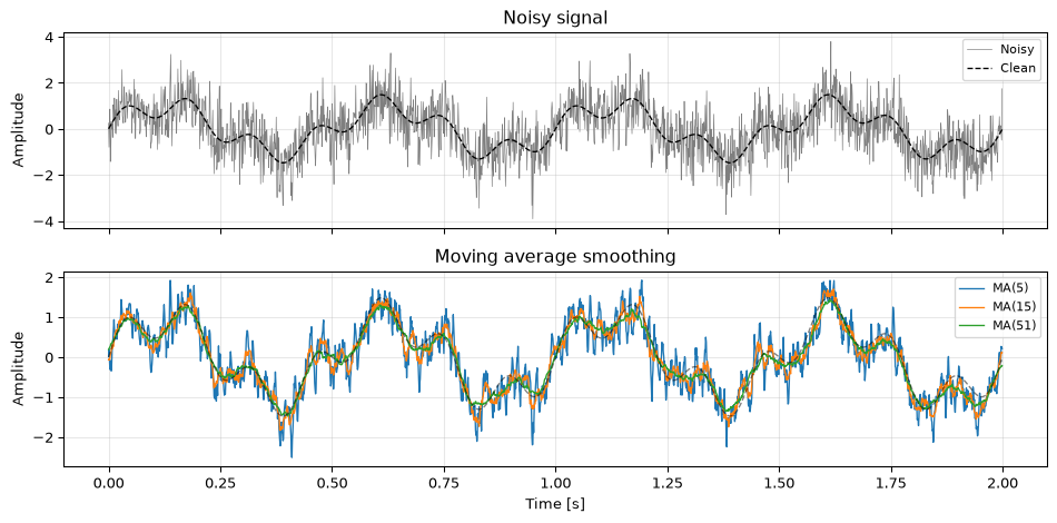
The simplest smoother. An $N$-point moving average replaces each sample with the mean of its $N$ neighbours:

\[y[n] = \frac{1}{N} \sum_{k=0}^{N-1} x[n-k]\]

This is a causal FIR filter with uniform coefficients $h[k] = 1/N$. Its frequency response is a sinc-like shape with the first null at $f_s / N$. The moving average is optimal for reducing random white noise while preserving a sharp step response, but it is a poor lowpass filter in the frequency-domain sense, with only 13 dB of sidelobe rejection regardless of $N$.

import numpy as np
import matplotlib.pyplot as plt
from scipy import signal as sig

# Noisy test signal: slow sine + noise
rng = np.random.default_rng(42)
fs = 1000
t = np.arange(2000) / fs
x_clean = np.sin(2 * np.pi * 2 * t) + 0.5 * np.sin(2 * np.pi * 7 * t)
x = x_clean + 0.8 * rng.standard_normal(len(t))

fig, axes = plt.subplots(2, 1, figsize=(10, 5), sharex=True)
axes[0].plot(t, x, 'C7', linewidth=0.5, label='Noisy')
axes[0].plot(t, x_clean, 'k--', linewidth=1, label='Clean')
axes[0].legend(fontsize=8)
axes[0].set_ylabel('Amplitude')
axes[0].set_title('Noisy signal')

for N in [5, 15, 51]:
    h = np.ones(N) / N
    y = np.convolve(x, h, mode='same')
    axes[1].plot(t, y, linewidth=1, label=f'MA({N})')

axes[1].plot(t, x_clean, 'k--', linewidth=1, alpha=0.5)
axes[1].set_xlabel('Time [s]')
axes[1].set_ylabel('Amplitude')
axes[1].set_title('Moving average smoothing')
axes[1].legend(fontsize=8)
for ax in axes:
    ax.grid(True, alpha=0.3)
fig.tight_layout()
plt.show()

Figure 1: Moving average smoothing: a 51-point MA filter removes high-frequency noise from a noisy sinusoid.

Longer windows remove more noise but also attenuate signal components and introduce lag. For the causal moving average, the group delay is $(N-1)/2$ samples.

Savitzky-Golay filter

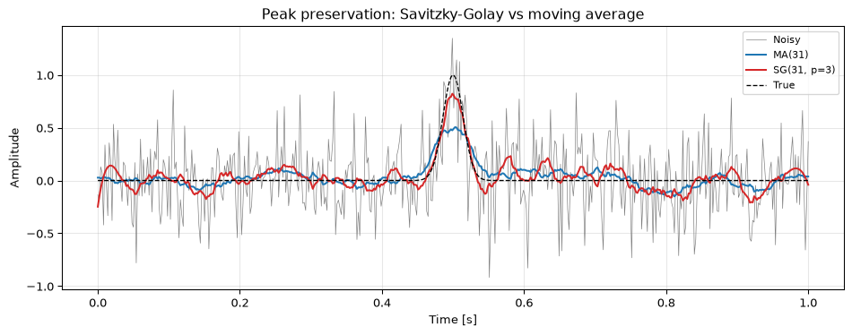
The Savitzky-Golay filter fits a local polynomial of degree $p$ to a window of $N$ points, then evaluates the polynomial at the centre of the window. Because a polynomial of degree $p$ passes through the filter unchanged, Savitzky-Golay preserves peaks, shoulders, and other features better than a moving average of the same length.

The filter coefficients are the result of a least-squares polynomial fit, computed once for given $N$ and $p$. SciPy provides savgol_filter with optional derivative computation, a useful side benefit, since the fitted polynomial can be differentiated analytically.

from scipy.signal import savgol_filter

# Signal with a sharp peak
t2 = np.linspace(0, 1, 500)
x_peak = np.exp(-((t2 - 0.5) / 0.02)**2) + 0.3 * rng.standard_normal(len(t2))

y_ma = np.convolve(x_peak, np.ones(31)/31, mode='same')
y_sg = savgol_filter(x_peak, window_length=31, polyorder=3)

fig, ax = plt.subplots(figsize=(10, 4))
ax.plot(t2, x_peak, 'C7', linewidth=0.5, label='Noisy')
ax.plot(t2, y_ma, 'C0', linewidth=1.5, label='MA(31)')
ax.plot(t2, y_sg, 'C3', linewidth=1.5, label='SG(31, p=3)')
ax.plot(t2, np.exp(-((t2 - 0.5) / 0.02)**2), 'k--', linewidth=1, label='True')
ax.set_xlabel('Time [s]')
ax.set_ylabel('Amplitude')
ax.legend(fontsize=8)
ax.grid(True, alpha=0.3)
ax.set_title('Peak preservation: Savitzky-Golay vs moving average')
fig.tight_layout()
plt.show()

Figure 2: Savitzky-Golay vs moving average on a signal with a sharp peak. The SG filter (polynomial order 3) preserves peak height and shape; the moving average flattens it.

Window length vs polynomial order

If $p$ is too close to $N-1$, the filter does almost no smoothing: it starts fitting the noise. A good starting point is $p = 2$ or $3$ with $N$ at least 3 to 5 times larger than $p + 1$. There is no universally optimal choice; it depends on the noise level and the features you want to preserve.

Exponential smoothing

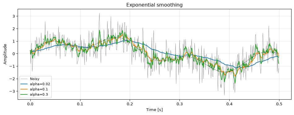
Exponential smoothing applies a first-order IIR filter:

\[y[n] = \alpha\, x[n] + (1 - \alpha)\, y[n-1], \quad 0 < \alpha \le 1\]

The smoothing factor $\alpha$ controls the trade-off: small $\alpha$ gives heavy smoothing (long memory), large $\alpha$ tracks the input closely. The impulse response decays geometrically: $h[n] = \alpha (1-\alpha)^n$, so recent samples contribute more than old ones.

The main advantage over moving averages is constant memory: only one state variable $y[n-1]$ is needed regardless of the effective smoothing window. This makes exponential smoothing popular in embedded systems and streaming applications.

fig, ax = plt.subplots(figsize=(10, 4))
ax.plot(t[:500], x[:500], 'C7', linewidth=0.5, label='Noisy')

for alpha in [0.02, 0.1, 0.3]:
    y_exp = np.zeros(500)
    y_exp[0] = x[0]
    for n in range(1, 500):
        y_exp[n] = alpha * x[n] + (1 - alpha) * y_exp[n-1]
    ax.plot(t[:500], y_exp, linewidth=1.5, label=f'alpha={alpha}')

ax.plot(t[:500], x_clean[:500], 'k--', linewidth=1, alpha=0.5)
ax.set_xlabel('Time [s]')
ax.set_ylabel('Amplitude')
ax.legend(fontsize=8)
ax.grid(True, alpha=0.3)
ax.set_title('Exponential smoothing')
fig.tight_layout()
plt.show()

Figure 3: Exponential smoothing with different values of alpha. Smaller alpha gives heavier smoothing but more lag.

The equivalent time constant is $\tau = -1 / \ln(1 - \alpha)$ samples. To relate $\alpha$ to a cutoff frequency: $\alpha = 1 - e^{-2\pi f_c / f_s}$.

Kernel smoothing

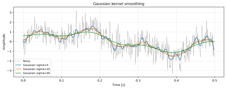
All the methods above are special cases of convolution with a kernel. Kernel smoothing generalises this by allowing any smooth, symmetric kernel: Gaussian, Epanechnikov, tricube, etc. The Gaussian kernel is the most common:

\[h[n] = \frac{1}{\sqrt{2\pi}\sigma} \exp\!\left(-\frac{n^2}{2\sigma^2}\right)\]

where $\sigma$ controls the bandwidth. Gaussian smoothing has the useful property that it never introduces new extrema (it only removes them) and its frequency response is also Gaussian: no sidelobes at all.

from scipy.ndimage import gaussian_filter1d

fig, ax = plt.subplots(figsize=(10, 4))
ax.plot(t[:500], x[:500], 'C7', linewidth=0.5, label='Noisy')

for sigma in [3, 10, 30]:
    y_gauss = gaussian_filter1d(x[:500], sigma=sigma)
    ax.plot(t[:500], y_gauss, linewidth=1.5, label=f'Gaussian sigma={sigma}')

ax.plot(t[:500], x_clean[:500], 'k--', linewidth=1, alpha=0.5)
ax.set_xlabel('Time [s]')
ax.set_ylabel('Amplitude')
ax.legend(fontsize=8)
ax.grid(True, alpha=0.3)
ax.set_title('Gaussian kernel smoothing')
fig.tight_layout()
plt.show()

Figure 4: Gaussian kernel smoothing at different bandwidths compared to a moving average of similar effective width.

When to use what

Method	Preserves peaks?	Constant memory?	Real-time?	Best for
Moving average	No	No ($N$ samples)	Yes	White noise on step-like signals
Savitzky-Golay	Yes	No ($N$ samples)	Yes	Preserving peak shape, derivatives
Exponential	No	Yes (1 sample)	Yes	Streaming, embedded systems
Gaussian kernel	No	No	Batch	Smooth, sidelobe-free suppression

The fundamental trade-off across all methods is smoothness vs lag. More aggressive smoothing removes more noise but delays features and can distort their shape. There is no way around this: it is a consequence of the uncertainty principle relating time and frequency resolution.

For real-time applications, exponential smoothing or short causal moving averages are the practical choices. For offline analysis where you can process the entire signal at once, Savitzky-Golay or Gaussian kernels usually give better results because they can be applied symmetrically (zero phase delay).

Tip

If you need smoothing without phase distortion, combine any of these methods with zero-phase filtering: apply the filter forward and backward.

Open questions

Adaptive smoothing bandwidth. A fixed smoothing window is a compromise: too short in quiet regions (not enough noise reduction), too long near transients (smears sharp features). Adaptive methods that vary the smoothing bandwidth based on local signal characteristics exist: Stein’s unbiased risk estimate (SURE) and cross-validation-based approaches are theoretically appealing but add significant complexity. In practice, most people just pick a window length by eye and move on.

Edge effects. All finite-window smoothers have boundary problems: what do you do at the start and end of the signal where the full window is not available? Common strategies include mirror padding, constant extrapolation, or shrinking the window. None is fully satisfactory, and the choice can significantly affect results near the edges.

References

Ballerini, M., N. Cabibbo, R. Candelier, A. Cavagna, E. Cisbani, I. Giardina, V. Lecomte, et al. 2008. “Interaction Ruling Animal Collective Behavior Depends on Topological Rather Than Metric Distance.” Proceedings of the National Academy of Sciences 105 (4): 1232–37.

Reynolds, Craig W. 1987. “Flocks, Herds and Schools: A Distributed Behavioral Model.” In Proceedings of the 14th Annual Conference on Computer Graphics and Interactive Techniques (SIGGRAPH), 25–34.

--- title: "Smoothing" subtitle: "Moving averages and beyond" --- ::: {.callout-tip title="Nature's smoothing filter" appearance="simple"} A flock of starlings moves as one, thousands of birds producing smooth, coordinated motion from individually noisy heading decisions. Empirical studies show each bird tracks approximately 6-7 nearest neighbours [@ballerini2008interaction], averaging their directions, a spatial moving average that filters out individual jitter. Craig Reynolds formalised this as a computational model [@reynolds1987flocks], demonstrating that simple local averaging rules produce the complex collective patterns we observe. ::: Sensor data is noisy. Before you can extract meaningful features (peaks, trends, zero crossings) you typically need to smooth the signal. For embedded implementations (EMA and moving average with circular buffer on ESP32-S3 and STM32F4), see [Smoothing on Hardware](embedded.qmd). The question is never *whether* to smooth, but *how much* and *with what method*. Every smoothing technique trades off noise suppression against signal distortion, and the right choice depends on what you plan to do with the signal afterwards. This page covers four approaches: moving averages, Savitzky-Golay filters, exponential smoothing, and kernel smoothing. Each has a sweet spot. None is universally best. ::: {.callout-note title="Prerequisites"} This topic assumes familiarity with [discrete-time systems](../../basics/02-discrete-time.qmd) (convolution, FIR filters) and [frequency-domain analysis](../../basics/05-frequency-domain.qmd). The moving average is introduced in [Chapter 2](../../basics/02-discrete-time.qmd) as a basic FIR filter. This page extends the idea. ::: --- ## Moving average The simplest smoother. An $N$-point moving average replaces each sample with the mean of its $N$ neighbours: $$y[n] = \frac{1}{N} \sum_{k=0}^{N-1} x[n-k]$$ This is a causal FIR filter with uniform coefficients $h[k] = 1/N$. Its frequency response is a sinc-like shape with the first null at $f_s / N$. The moving average is optimal for reducing random white noise while preserving a sharp step response, but it is a poor lowpass filter in the frequency-domain sense, with only 13 dB of sidelobe rejection regardless of $N$. ```{python} #| label: fig-smoothing-demo #| fig-cap: "Moving average smoothing: a 51-point MA filter removes high-frequency noise from a noisy sinusoid." import numpy as np import matplotlib.pyplot as plt from scipy import signal as sig # Noisy test signal: slow sine + noise rng = np.random.default_rng(42) fs = 1000 t = np.arange(2000) / fs x_clean = np.sin(2 * np.pi * 2 * t) + 0.5 * np.sin(2 * np.pi * 7 * t) x = x_clean + 0.8 * rng.standard_normal(len(t)) fig, axes = plt.subplots(2, 1, figsize=(10, 5), sharex=True) axes[0].plot(t, x, 'C7', linewidth=0.5, label='Noisy') axes[0].plot(t, x_clean, 'k--', linewidth=1, label='Clean') axes[0].legend(fontsize=8) axes[0].set_ylabel('Amplitude') axes[0].set_title('Noisy signal') for N in [5, 15, 51]: h = np.ones(N) / N y = np.convolve(x, h, mode='same') axes[1].plot(t, y, linewidth=1, label=f'MA({N})') axes[1].plot(t, x_clean, 'k--', linewidth=1, alpha=0.5) axes[1].set_xlabel('Time [s]') axes[1].set_ylabel('Amplitude') axes[1].set_title('Moving average smoothing') axes[1].legend(fontsize=8) for ax in axes: ax.grid(True, alpha=0.3) fig.tight_layout() plt.show() ``` Longer windows remove more noise but also attenuate signal components and introduce lag. For the causal moving average, the group delay is $(N-1)/2$ samples. --- ## Savitzky-Golay filter The Savitzky-Golay filter fits a local polynomial of degree $p$ to a window of $N$ points, then evaluates the polynomial at the centre of the window. Because a polynomial of degree $p$ passes through the filter unchanged, Savitzky-Golay preserves peaks, shoulders, and other features better than a moving average of the same length. The filter coefficients are the result of a least-squares polynomial fit, computed once for given $N$ and $p$. SciPy provides `savgol_filter` with optional derivative computation, a useful side benefit, since the fitted polynomial can be differentiated analytically. ```{python} #| label: fig-savgol #| fig-cap: "Savitzky-Golay vs moving average on a signal with a sharp peak. The SG filter (polynomial order 3) preserves peak height and shape; the moving average flattens it." from scipy.signal import savgol_filter # Signal with a sharp peak t2 = np.linspace(0, 1, 500) x_peak = np.exp(-((t2 - 0.5) / 0.02)**2) + 0.3 * rng.standard_normal(len(t2)) y_ma = np.convolve(x_peak, np.ones(31)/31, mode='same') y_sg = savgol_filter(x_peak, window_length=31, polyorder=3) fig, ax = plt.subplots(figsize=(10, 4)) ax.plot(t2, x_peak, 'C7', linewidth=0.5, label='Noisy') ax.plot(t2, y_ma, 'C0', linewidth=1.5, label='MA(31)') ax.plot(t2, y_sg, 'C3', linewidth=1.5, label='SG(31, p=3)') ax.plot(t2, np.exp(-((t2 - 0.5) / 0.02)**2), 'k--', linewidth=1, label='True') ax.set_xlabel('Time [s]') ax.set_ylabel('Amplitude') ax.legend(fontsize=8) ax.grid(True, alpha=0.3) ax.set_title('Peak preservation: Savitzky-Golay vs moving average') fig.tight_layout() plt.show() ``` ::: {.callout-warning title="Window length vs polynomial order"} If $p$ is too close to $N-1$, the filter does almost no smoothing: it starts fitting the noise. A good starting point is $p = 2$ or $3$ with $N$ at least 3 to 5 times larger than $p + 1$. There is no universally optimal choice; it depends on the noise level and the features you want to preserve. ::: --- ## Exponential smoothing Exponential smoothing applies a first-order IIR filter: $$y[n] = \alpha\, x[n] + (1 - \alpha)\, y[n-1], \quad 0 < \alpha \le 1$$ The smoothing factor $\alpha$ controls the trade-off: small $\alpha$ gives heavy smoothing (long memory), large $\alpha$ tracks the input closely. The impulse response decays geometrically: $h[n] = \alpha (1-\alpha)^n$, so recent samples contribute more than old ones. The main advantage over moving averages is **constant memory**: only one state variable $y[n-1]$ is needed regardless of the effective smoothing window. This makes exponential smoothing popular in embedded systems and streaming applications. ```{python} #| label: fig-exponential #| fig-cap: "Exponential smoothing with different values of alpha. Smaller alpha gives heavier smoothing but more lag." fig, ax = plt.subplots(figsize=(10, 4)) ax.plot(t[:500], x[:500], 'C7', linewidth=0.5, label='Noisy') for alpha in [0.02, 0.1, 0.3]: y_exp = np.zeros(500) y_exp[0] = x[0] for n in range(1, 500): y_exp[n] = alpha * x[n] + (1 - alpha) * y_exp[n-1] ax.plot(t[:500], y_exp, linewidth=1.5, label=f'alpha={alpha}') ax.plot(t[:500], x_clean[:500], 'k--', linewidth=1, alpha=0.5) ax.set_xlabel('Time [s]') ax.set_ylabel('Amplitude') ax.legend(fontsize=8) ax.grid(True, alpha=0.3) ax.set_title('Exponential smoothing') fig.tight_layout() plt.show() ``` The equivalent time constant is $\tau = -1 / \ln(1 - \alpha)$ samples. To relate $\alpha$ to a cutoff frequency: $\alpha = 1 - e^{-2\pi f_c / f_s}$. --- ## Kernel smoothing All the methods above are special cases of convolution with a kernel. **Kernel smoothing** generalises this by allowing any smooth, symmetric kernel: Gaussian, Epanechnikov, tricube, etc. The Gaussian kernel is the most common: $$h[n] = \frac{1}{\sqrt{2\pi}\sigma} \exp\!\left(-\frac{n^2}{2\sigma^2}\right)$$ where $\sigma$ controls the bandwidth. Gaussian smoothing has the useful property that it never introduces new extrema (it only removes them) and its frequency response is also Gaussian: no sidelobes at all. ```{python} #| label: fig-kernel #| fig-cap: "Gaussian kernel smoothing at different bandwidths compared to a moving average of similar effective width." from scipy.ndimage import gaussian_filter1d fig, ax = plt.subplots(figsize=(10, 4)) ax.plot(t[:500], x[:500], 'C7', linewidth=0.5, label='Noisy') for sigma in [3, 10, 30]: y_gauss = gaussian_filter1d(x[:500], sigma=sigma) ax.plot(t[:500], y_gauss, linewidth=1.5, label=f'Gaussian sigma={sigma}') ax.plot(t[:500], x_clean[:500], 'k--', linewidth=1, alpha=0.5) ax.set_xlabel('Time [s]') ax.set_ylabel('Amplitude') ax.legend(fontsize=8) ax.grid(True, alpha=0.3) ax.set_title('Gaussian kernel smoothing') fig.tight_layout() plt.show() ``` --- ## When to use what | Method | Preserves peaks? | Constant memory? | Real-time? | Best for | |--------|:-:|:-:|:-:|------| | Moving average | No | No ($N$ samples) | Yes | White noise on step-like signals | | Savitzky-Golay | Yes | No ($N$ samples) | Yes | Preserving peak shape, derivatives | | Exponential | No | Yes (1 sample) | Yes | Streaming, embedded systems | | Gaussian kernel | No | No | Batch | Smooth, sidelobe-free suppression | The fundamental trade-off across all methods is **smoothness vs lag**. More aggressive smoothing removes more noise but delays features and can distort their shape. There is no way around this: it is a consequence of the uncertainty principle relating time and frequency resolution. For real-time applications, exponential smoothing or short causal moving averages are the practical choices. For offline analysis where you can process the entire signal at once, Savitzky-Golay or Gaussian kernels usually give better results because they can be applied symmetrically (zero phase delay). ::: {.callout-tip} If you need smoothing without phase distortion, combine any of these methods with [zero-phase filtering](../zero-phase/index.qmd): apply the filter forward and backward. ::: --- ## Open questions **Adaptive smoothing bandwidth.** A fixed smoothing window is a compromise: too short in quiet regions (not enough noise reduction), too long near transients (smears sharp features). Adaptive methods that vary the smoothing bandwidth based on local signal characteristics exist: Stein's unbiased risk estimate (SURE) and cross-validation-based approaches are theoretically appealing but add significant complexity. In practice, most people just pick a window length by eye and move on. **Edge effects.** All finite-window smoothers have boundary problems: what do you do at the start and end of the signal where the full window is not available? Common strategies include mirror padding, constant extrapolation, or shrinking the window. None is fully satisfactory, and the choice can significantly affect results near the edges.