From raw audio to ‘you’re 12 cents sharp’: a guided DSP build
Build a working guitar tuner in Python, from raw audio to precise pitch and tuning feedback. This project ties together bandpass filtering, spectral analysis, autocorrelation-based pitch detection, and note matching, concepts from frequency domain analysis, filter design, and the pitch detection topic.
By the end you will have a function that takes in a signal, estimates the fundamental frequency, finds the nearest musical note, and reports how many cents sharp or flat you are.
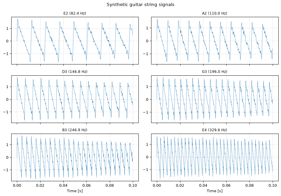
A real guitar string produces a fundamental frequency plus harmonics at integer multiples (2x, 3x, 4x, …), with each harmonic weaker than the last. We will synthesise this, add a touch of detuning for realism, and mix in some noise. This gives us repeatable test data without needing a microphone.
Task: Write a function make_guitar_string(f0, fs, duration, snr_db) that generates a synthetic plucked-string signal with harmonics, slight random detuning, and additive noise at the specified SNR.
Solution
import numpy as npimport matplotlib.pyplot as pltdef make_guitar_string(f0, fs=8000, duration=1.0, snr_db=20, rng=None):"""Synthesise a guitar string signal with harmonics, detuning, and noise. Parameters ---------- f0 : float Fundamental frequency in Hz. fs : int Sampling rate in Hz. duration : float Signal length in seconds. snr_db : float Signal-to-noise ratio in dB. rng : np.random.Generator or None Random number generator (for reproducibility). Returns ------- t : ndarray — time vector x : ndarray — noisy guitar string signal """if rng isNone: rng = np.random.default_rng(42) t = np.arange(int(fs * duration)) / fs signal = np.zeros_like(t)# Add harmonics up to Nyquist, with decreasing amplitude and slight detuning n_harmonics =int(fs /2/ f0)for k inrange(1, min(n_harmonics, 8) +1): detune =1+ rng.uniform(-0.001, 0.001) # up to 0.1% detuning amp =1.0/ k # amplitude falls as 1/k signal += amp * np.sin(2* np.pi * f0 * k * detune * t)# Simple exponential decay envelope (plucked string) envelope = np.exp(-2* t) signal *= envelope# Add noise at specified SNR sig_power = np.mean(signal**2) noise_power = sig_power / (10** (snr_db /10)) noise = rng.standard_normal(len(t)) * np.sqrt(noise_power)return t, signal + noise# Generate all six stringsrng = np.random.default_rng(42)fs =8000string_freqs = {'E2': 82.41, 'A2': 110.00, 'D3': 146.83,'G3': 196.00, 'B3': 246.94, 'E4': 329.63,}fig, axes = plt.subplots(3, 2, figsize=(10, 7), sharex=True)for ax, (name, f0) inzip(axes.flat, string_freqs.items()): t, x = make_guitar_string(f0, fs=fs, duration=0.5, snr_db=20, rng=rng) ax.plot(t[:800], x[:800], linewidth=0.5) ax.set_title(f'{name} ({f0:.1f} Hz)', fontsize=9) ax.grid(True, alpha=0.3)axes[-1, 0].set_xlabel('Time [s]')axes[-1, 1].set_xlabel('Time [s]')fig.suptitle('Synthetic guitar string signals', fontsize=11)fig.tight_layout()plt.show()
Step 2: Bandpass filter
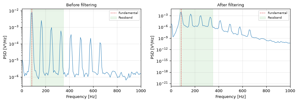
Guitar fundamentals range from about 82 Hz (low E) to 330 Hz (high E). We want to remove low-frequency hum and high-frequency harmonics that could confuse the pitch detector. A bandpass filter from 70 to 350 Hz keeps all fundamentals while rejecting everything else.
Task: Design a 4th-order Butterworth bandpass filter using second-order sections (SOS) and apply it with sosfilt. Plot the spectrum before and after filtering for the low E string.
Harmonics above the 350 Hz passband edge are attenuated, and low-frequency noise below 70 Hz is removed. (The passband is deliberately wide enough to pass every string’s fundamental up to high E at 330 Hz, so for the low-E string at 82 Hz the first few harmonics (2x, 3x, 4x at 165, 247, 330 Hz) still fall inside it; only the 5th harmonic and above, from ~412 Hz, are removed.) This gives the autocorrelation pitch detector a cleaner signal to work with.
Step 3: Pitch detection via autocorrelation
The autocorrelation of a periodic signal has peaks at multiples of the period. By finding the first prominent peak after the zero-lag peak, we can estimate the fundamental period, and from that, the fundamental frequency.
Why autocorrelation? Because it naturally locks onto the fundamental period even when the harmonics are stronger than the fundamental. This is a known advantage over simpler methods like zero-crossing counting (see pitch detection for the full comparison).
The estimates should be within a few Hz of the true fundamentals. The confidence value indicates how strongly periodic the signal is: values above 0.8 indicate a reliable estimate.
Step 4: Note matching and cents deviation
Musicians don’t think in Hz. They think in note names and “how far off am I?” In equal temperament, every note has a well-defined frequency:
\[f_{\text{note}} = 440 \times 2^{(n - 69)/12}\]
where \(n\) is the MIDI note number (A4 = 69). The cent is a logarithmic unit: 100 cents = 1 semitone. The deviation in cents between an estimated frequency and a reference is:
\[\Delta c = 1200 \cdot \log_2\!\left(\frac{f_{\text{est}}}{f_{\text{note}}}\right)\]
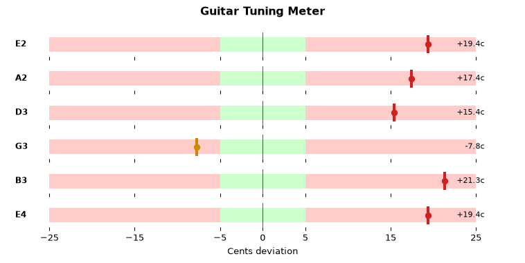
A deviation of \(\pm 5\) cents is inaudible to most people. Beyond \(\pm 15\) cents, even casual listeners notice the string is out of tune.
Task: Write freq_to_note(f) that returns the nearest note name and the cents deviation.
Solution
def freq_to_note(f):"""Convert frequency to nearest note name and cents deviation. Parameters ---------- f : float Frequency in Hz. Returns ------- name : str Note name with octave (e.g. 'A4', 'E2'). cents : float Deviation from the nearest note in cents. """if f <=0:return'---', 0.0# MIDI note number (continuous) midi =69+12* np.log2(f /440) midi_round =round(midi) cents = (midi - midi_round) *100 note_names = ['C', 'C#', 'D', 'D#', 'E', 'F','F#', 'G', 'G#', 'A', 'A#', 'B'] name = note_names[midi_round %12] +str(midi_round //12-1)return name, cents# Test with the guitar string frequenciesprint(f"{'Freq (Hz)':>10}{'Note':>5}{'Cents':>8}")print('-'*28)for f in string_freqs.values(): note, cents = freq_to_note(f)print(f"{f:>10.2f}{note:>5}{cents:>+8.1f}")# Also test with a detuned frequencyf_detuned =112.5# A2 is 110 Hz, so this is sharpnote, cents = freq_to_note(f_detuned)print(f"\n{f_detuned} Hz -> {note}{cents:+.1f} cents")
With a confidence threshold around 0.5, the tuner can flag uncertain results and ask the player to pluck again more firmly or move closer to the microphone.
Harmonics stronger than fundamental
Guitar strings often produce harmonics that are louder than the fundamental, especially on wound strings (E2, A2, D3). Why does autocorrelation still find the correct pitch?
Explanation
The autocorrelation of a periodic signal always has its strongest peak (after the zero-lag peak) at the fundamental period, regardless of which harmonic has the most energy. This is because all harmonics are periodic at the fundamental period: the 2nd harmonic completes exactly 2 cycles, the 3rd completes 3 cycles, and so on. Their contributions all reinforce at the fundamental lag.
This is one of the main reasons autocorrelation is preferred over spectral peak picking for guitar tuners. A naive “find the tallest spectral peak” approach would often return a harmonic frequency, reporting the string as an octave (or more) too high.
Short signals: minimum frame length
Task: How short can the analysis frame be before pitch detection fails for the low E string?
For the low E string (82 Hz), one full period is about 12 ms. The autocorrelation needs at least two full periods to find a peak, so frame lengths below ~25 ms become unreliable. As a rule of thumb: the minimum frame length is \(2 / f_{\min}\) seconds, and for a guitar tuner with \(f_{\min} = 82\) Hz, that is about 25 ms.
Reflection questions
These are open-ended. Think about them before checking the discussion.
Why autocorrelation over zero-crossing? A guitar signal has many zero crossings per period (from the harmonics), so zero-crossing counting would overestimate the frequency. Autocorrelation finds the true period by looking for self-similarity, which is robust to harmonic content. See the pitch detection topic for a detailed comparison.
Minimum window length for low E. The low E string at 82 Hz has a period of \(1/82 \approx 12.2\) ms. The autocorrelation needs at least 2 periods to identify the peak, so the minimum useful window is about 25 ms. For comfortable margin, 50 ms (4 periods) is better. This is a concrete example of the frequency resolution vs. time resolution trade-off from Ch5.
Extending to a chromatic tuner. Remove the bandpass filter (or widen it to 20–5000 Hz), extend the fmin/fmax range in estimate_pitch, and the freq_to_note function already handles all 12 notes. The main challenge is dealing with a wider frequency range in the autocorrelation lag search.
Real-time embedded version. On a microcontroller, you would: (a) replace the FFT-based autocorrelation with a direct lag computation (or use CMSIS-DSP), (b) implement the bandpass as a cascade of biquad sections for numerical stability, and (c) process fixed-size frames from a circular buffer fed by an ADC interrupt. The biquad embedded page covers the implementation details.
Source Code
---title: "Project: Build a Guitar Tuner"subtitle: "From raw audio to 'you're 12 cents sharp': a guided DSP build"---Build a working guitar tuner in Python, from raw audio to precise pitch and tuning feedback. This project ties together bandpass filtering, spectral analysis, autocorrelation-based pitch detection, and note matching, concepts from [frequency domain analysis](../basics/05-frequency-domain.qmd), [filter design](../basics/06-filter-design.qmd), and the [pitch detection](../topics/pitch-detection/index.qmd) topic.By the end you will have a function that takes in a signal, estimates the fundamental frequency, finds the nearest musical note, and reports how many cents sharp or flat you are.::: {.callout-note title="Prerequisites"}This project draws on concepts from [Chapter 3: Noise and SNR](../basics/03-noise-snr.qmd) (signal power, SNR), [Chapter 5: Frequency domain](../basics/05-frequency-domain.qmd) (DFT, spectral analysis), and [Chapter 6: Filter design](../basics/06-filter-design.qmd) (Butterworth bandpass, SOS form). The [pitch detection](../topics/pitch-detection/index.qmd) topic covers the theory in more depth.:::### Guitar string reference| String | Note | Frequency (Hz) ||--------|------|-----------------|| 6 (low E) | E2 | 82.41 || 5 | A2 | 110.00 || 4 | D3 | 146.83 || 3 | G3 | 196.00 || 2 | B3 | 246.94 || 1 (high E) | E4 | 329.63 |---## Step 1: Generate test signalsA real guitar string produces a fundamental frequency plus harmonics at integer multiples (2x, 3x, 4x, ...), with each harmonic weaker than the last. We will synthesise this, add a touch of detuning for realism, and mix in some noise. This gives us repeatable test data without needing a microphone.**Task:** Write a function `make_guitar_string(f0, fs, duration, snr_db)` that generates a synthetic plucked-string signal with harmonics, slight random detuning, and additive noise at the specified SNR.::: {.callout-note collapse="true" title="Solution"}```{python}import numpy as npimport matplotlib.pyplot as pltdef make_guitar_string(f0, fs=8000, duration=1.0, snr_db=20, rng=None):"""Synthesise a guitar string signal with harmonics, detuning, and noise. Parameters ---------- f0 : float Fundamental frequency in Hz. fs : int Sampling rate in Hz. duration : float Signal length in seconds. snr_db : float Signal-to-noise ratio in dB. rng : np.random.Generator or None Random number generator (for reproducibility). Returns ------- t : ndarray — time vector x : ndarray — noisy guitar string signal """if rng isNone: rng = np.random.default_rng(42) t = np.arange(int(fs * duration)) / fs signal = np.zeros_like(t)# Add harmonics up to Nyquist, with decreasing amplitude and slight detuning n_harmonics =int(fs /2/ f0)for k inrange(1, min(n_harmonics, 8) +1): detune =1+ rng.uniform(-0.001, 0.001) # up to 0.1% detuning amp =1.0/ k # amplitude falls as 1/k signal += amp * np.sin(2* np.pi * f0 * k * detune * t)# Simple exponential decay envelope (plucked string) envelope = np.exp(-2* t) signal *= envelope# Add noise at specified SNR sig_power = np.mean(signal**2) noise_power = sig_power / (10** (snr_db /10)) noise = rng.standard_normal(len(t)) * np.sqrt(noise_power)return t, signal + noise# Generate all six stringsrng = np.random.default_rng(42)fs =8000string_freqs = {'E2': 82.41, 'A2': 110.00, 'D3': 146.83,'G3': 196.00, 'B3': 246.94, 'E4': 329.63,}fig, axes = plt.subplots(3, 2, figsize=(10, 7), sharex=True)for ax, (name, f0) inzip(axes.flat, string_freqs.items()): t, x = make_guitar_string(f0, fs=fs, duration=0.5, snr_db=20, rng=rng) ax.plot(t[:800], x[:800], linewidth=0.5) ax.set_title(f'{name} ({f0:.1f} Hz)', fontsize=9) ax.grid(True, alpha=0.3)axes[-1, 0].set_xlabel('Time [s]')axes[-1, 1].set_xlabel('Time [s]')fig.suptitle('Synthetic guitar string signals', fontsize=11)fig.tight_layout()plt.show()```:::---## Step 2: Bandpass filterGuitar fundamentals range from about 82 Hz (low E) to 330 Hz (high E). We want to remove low-frequency hum and high-frequency harmonics that could confuse the pitch detector. A bandpass filter from 70 to 350 Hz keeps all fundamentals while rejecting everything else.**Task:** Design a 4th-order Butterworth bandpass filter using second-order sections (SOS) and apply it with `sosfilt`. Plot the spectrum before and after filtering for the low E string.*Concepts used:* [filter design](../basics/06-filter-design.qmd), [biquad sections](../topics/biquad/index.qmd).::: {.callout-note collapse="true" title="Solution"}```{python}from scipy.signal import butter, sosfilt, welch# Design bandpass filter: 70-350 Hz covers all guitar fundamentalssos = butter(4, [70, 350], btype='band', fs=fs, output='sos')# Generate a test signal (low E string — hardest case, lowest frequency)rng_test = np.random.default_rng(42)t, x = make_guitar_string(82.41, fs=fs, duration=1.0, snr_db=15, rng=rng_test)# Apply filterx_filt = sosfilt(sos, x)# Compare spectrafig, axes = plt.subplots(1, 2, figsize=(10, 3.5))for ax, (sig, label) inzip(axes, [(x, 'Before filtering'), (x_filt, 'After filtering')]): f, psd = welch(sig, fs, nperseg=1024) ax.semilogy(f, psd, linewidth=0.8) ax.axvline(82.41, color='C3', linewidth=0.8, linestyle='--', label='Fundamental') ax.axvspan(70, 350, alpha=0.1, color='C2', label='Passband') ax.set_xlabel('Frequency [Hz]') ax.set_ylabel('PSD [V²/Hz]') ax.set_title(label, fontsize=10) ax.legend(fontsize=7) ax.grid(True, alpha=0.3) ax.set_xlim(0, 1000)fig.tight_layout()plt.show()```Harmonics above the 350 Hz passband edge are attenuated, and low-frequency noise below 70 Hz is removed. (The passband is deliberately wide enough to pass every string's fundamental up to high E at 330 Hz, so for the low-E string at 82 Hz the first few harmonics (2x, 3x, 4x at 165, 247, 330 Hz) still fall inside it; only the 5th harmonic and above, from ~412 Hz, are removed.) This gives the autocorrelation pitch detector a cleaner signal to work with.:::---## Step 3: Pitch detection via autocorrelationThe autocorrelation of a periodic signal has peaks at multiples of the period. By finding the first prominent peak after the zero-lag peak, we can estimate the fundamental period, and from that, the fundamental frequency.Why autocorrelation? Because it naturally locks onto the **fundamental period** even when the harmonics are stronger than the fundamental. This is a known advantage over simpler methods like zero-crossing counting (see [pitch detection](../topics/pitch-detection/index.qmd) for the full comparison).**Task:** Implement autocorrelation-based pitch detection:1. Window a frame of the signal (e.g., 50 ms).2. Compute the (normalised) autocorrelation.3. Find the first prominent peak after the zero-lag peak.4. Convert lag to frequency: $\hat{f}_0 = f_s / \ell$ where $\ell$ is the lag in samples.::: {.callout-note collapse="true" title="Solution"}```{python}def estimate_pitch(x, fs, fmin=70, fmax=400):"""Estimate fundamental frequency using autocorrelation. Parameters ---------- x : ndarray Audio frame (windowed). fs : int Sampling rate. fmin, fmax : float Expected frequency range — limits the lag search window. Returns ------- f0 : float Estimated fundamental frequency in Hz. confidence : float Normalised autocorrelation peak height (0 to 1). """# Compute autocorrelation via FFT (fast) n =len(x) fft_x = np.fft.rfft(x, n=2*n) acf = np.fft.irfft(fft_x * np.conj(fft_x))[:n]# Normalise so zero-lag peak = 1if acf[0] ==0:return0.0, 0.0 acf = acf / acf[0]# Search for first peak in the valid lag range lag_min =int(fs / fmax) lag_max =int(fs / fmin) lag_max =min(lag_max, n -1)if lag_min >= lag_max:return0.0, 0.0 acf_search = acf[lag_min:lag_max +1]iflen(acf_search) ==0:return0.0, 0.0 peak_idx = np.argmax(acf_search) peak_lag = lag_min + peak_idx confidence = acf_search[peak_idx] f0 = fs / peak_lagreturn f0, confidence# Test on each stringrng_test = np.random.default_rng(42)frame_len =int(0.05* fs) # 50 ms frameprint(f"{'String':<8}{'True (Hz)':>10}{'Est. (Hz)':>10}{'Error (Hz)':>10}{'Conf.':>6}")print('-'*50)for name, f0_true in string_freqs.items(): t, x = make_guitar_string(f0_true, fs=fs, duration=0.5, snr_db=20, rng=rng_test) x_filt = sosfilt(sos, x) frame = x_filt[:frame_len] * np.hanning(frame_len) # window a frame f0_est, conf = estimate_pitch(frame, fs) err = f0_est - f0_trueprint(f"{name:<8}{f0_true:>10.2f}{f0_est:>10.2f}{err:>+10.2f}{conf:>6.3f}")```The estimates should be within a few Hz of the true fundamentals. The confidence value indicates how strongly periodic the signal is: values above 0.8 indicate a reliable estimate.:::---## Step 4: Note matching and cents deviationMusicians don't think in Hz. They think in note names and "how far off am I?" In equal temperament, every note has a well-defined frequency:$$f_{\text{note}} = 440 \times 2^{(n - 69)/12}$$where $n$ is the MIDI note number (A4 = 69). The **cent** is a logarithmic unit: 100 cents = 1 semitone. The deviation in cents between an estimated frequency and a reference is:$$\Delta c = 1200 \cdot \log_2\!\left(\frac{f_{\text{est}}}{f_{\text{note}}}\right)$$A deviation of $\pm 5$ cents is inaudible to most people. Beyond $\pm 15$ cents, even casual listeners notice the string is out of tune.**Task:** Write `freq_to_note(f)` that returns the nearest note name and the cents deviation.::: {.callout-note collapse="true" title="Solution"}```{python}def freq_to_note(f):"""Convert frequency to nearest note name and cents deviation. Parameters ---------- f : float Frequency in Hz. Returns ------- name : str Note name with octave (e.g. 'A4', 'E2'). cents : float Deviation from the nearest note in cents. """if f <=0:return'---', 0.0# MIDI note number (continuous) midi =69+12* np.log2(f /440) midi_round =round(midi) cents = (midi - midi_round) *100 note_names = ['C', 'C#', 'D', 'D#', 'E', 'F','F#', 'G', 'G#', 'A', 'A#', 'B'] name = note_names[midi_round %12] +str(midi_round //12-1)return name, cents# Test with the guitar string frequenciesprint(f"{'Freq (Hz)':>10}{'Note':>5}{'Cents':>8}")print('-'*28)for f in string_freqs.values(): note, cents = freq_to_note(f)print(f"{f:>10.2f}{note:>5}{cents:>+8.1f}")# Also test with a detuned frequencyf_detuned =112.5# A2 is 110 Hz, so this is sharpnote, cents = freq_to_note(f_detuned)print(f"\n{f_detuned} Hz -> {note}{cents:+.1f} cents")```:::---## Step 5: Put it all togetherNow we combine every piece into a single `tune()` function: signal in, note name and cents out.**Task:** Build the full pipeline and run it on all six strings. Display results in a table and create a visual tuning meter.::: {.callout-note collapse="true" title="Solution"}```{python}def tune(x, fs, sos):"""Full guitar tuner pipeline. Parameters ---------- x : ndarray Raw audio signal. fs : int Sampling rate. sos : ndarray Bandpass filter coefficients (second-order sections). Returns ------- note : str Nearest note name. cents : float Deviation in cents. f0 : float Estimated frequency in Hz. confidence : float Pitch detection confidence (0-1). """# 1. Bandpass filter x_filt = sosfilt(sos, x)# 2. Take a frame from the middle (skip filter transient) frame_len =int(0.05* fs) # 50 ms start =len(x_filt) //4# skip the first quarter (transient) frame = x_filt[start:start + frame_len]# 3. Window the frame frame = frame * np.hanning(len(frame))# 4. Estimate pitch f0, confidence = estimate_pitch(frame, fs)# 5. Map to note note, cents = freq_to_note(f0)return note, cents, f0, confidence# Run on all six stringsrng_test = np.random.default_rng(42)print(f"{'String':<8}{'Expected':>8}{'Got':>6}{'f0 (Hz)':>9} "f"{'Cents':>7}{'Conf.':>6}{'Verdict'}")print('-'*62)results = []for name, f0_true in string_freqs.items(): t, x = make_guitar_string(f0_true, fs=fs, duration=1.0, snr_db=20, rng=rng_test) note, cents, f0, conf = tune(x, fs, sos) verdict ='In tune'ifabs(cents) <5else ('Sharp'if cents >0else'Flat')print(f"{name:<8}{name:>8}{note:>6}{f0:>9.2f}{cents:>+7.1f}{conf:>6.3f}{verdict}") results.append((name, cents, conf))``````{python}#| fig-cap: "Tuning meter, green zone is within +/- 5 cents"fig, axes = plt.subplots(len(results), 1, figsize=(8, 4), sharex=True)for ax, (name, cents, conf) inzip(axes, results):# Draw the meter background ax.barh(0, 50, left=-25, height=0.6, color='#ffcccc', edgecolor='none') # red zone ax.barh(0, 10, left=-5, height=0.6, color='#ccffcc', edgecolor='none') # green zone# Draw the needle color ='#22aa22'ifabs(cents) <5else ('#cc8800'ifabs(cents) <15else'#cc2222') ax.plot(cents, 0, '|', markersize=20, color=color, markeredgewidth=3) ax.plot(cents, 0, 'o', markersize=6, color=color) ax.set_xlim(-30, 30) ax.set_ylim(-0.5, 0.5) ax.set_yticks([]) ax.text(-29, 0, f'{name}', fontsize=9, va='center', fontweight='bold') ax.text(26, 0, f'{cents:+.1f}c', fontsize=8, va='center', ha='right') ax.axvline(0, color='k', linewidth=0.5, linestyle='-') ax.set_frame_on(False)axes[-1].set_xlabel('Cents deviation')axes[-1].set_xticks([-25, -15, -5, 0, 5, 15, 25])fig.suptitle('Guitar Tuning Meter', fontsize=12, fontweight='bold')fig.tight_layout()plt.show()```:::---## Step 6: Handle edge casesA tuner that only works on clean synthetic signals is not very useful. What happens when things get difficult?### Low SNR**Task:** Run the tuner on a very noisy signal (SNR = 5 dB). What goes wrong? Add a confidence threshold to flag unreliable readings.::: {.callout-note collapse="true" title="Solution"}```{python}rng_noisy = np.random.default_rng(42)print("Low SNR test (5 dB):")print(f"{'String':<8}{'Note':>6}{'Cents':>7}{'Conf.':>6}{'Reliable?'}")print('-'*45)for name, f0_true in string_freqs.items(): t, x = make_guitar_string(f0_true, fs=fs, duration=1.0, snr_db=5, rng=rng_noisy) note, cents, f0, conf = tune(x, fs, sos) reliable = conf >0.5# confidence thresholdprint(f"{name:<8}{note:>6}{cents:>+7.1f}{conf:>6.3f}{'Yes'if reliable else'NO — retry'}")```With a confidence threshold around 0.5, the tuner can flag uncertain results and ask the player to pluck again more firmly or move closer to the microphone.:::### Harmonics stronger than fundamentalGuitar strings often produce harmonics that are louder than the fundamental, especially on wound strings (E2, A2, D3). Why does autocorrelation still find the correct pitch?::: {.callout-note collapse="true" title="Explanation"}The autocorrelation of a periodic signal always has its strongest peak (after the zero-lag peak) at the **fundamental period**, regardless of which harmonic has the most energy. This is because all harmonics are periodic at the fundamental period: the 2nd harmonic completes exactly 2 cycles, the 3rd completes 3 cycles, and so on. Their contributions all reinforce at the fundamental lag.This is one of the main reasons autocorrelation is preferred over spectral peak picking for guitar tuners. A naive "find the tallest spectral peak" approach would often return a harmonic frequency, reporting the string as an octave (or more) too high.:::### Short signals: minimum frame length**Task:** How short can the analysis frame be before pitch detection fails for the low E string?::: {.callout-note collapse="true" title="Solution"}```{python}rng_short = np.random.default_rng(42)t, x = make_guitar_string(82.41, fs=fs, duration=1.0, snr_db=20, rng=rng_short)x_filt = sosfilt(sos, x)frame_ms_list = [10, 15, 20, 25, 30, 40, 50, 75, 100]print(f"{'Frame (ms)':>10}{'f0 (Hz)':>9}{'Error (Hz)':>10}{'Conf.':>6}")print('-'*40)for frame_ms in frame_ms_list: frame_len =int(frame_ms /1000* fs) start =len(x_filt) //4 frame = x_filt[start:start + frame_len] * np.hanning(frame_len) f0, conf = estimate_pitch(frame, fs) err = f0 -82.41print(f"{frame_ms:>10}{f0:>9.2f}{err:>+10.2f}{conf:>6.3f}")```For the low E string (82 Hz), one full period is about 12 ms. The autocorrelation needs at least two full periods to find a peak, so frame lengths below ~25 ms become unreliable. As a rule of thumb: the minimum frame length is $2 / f_{\min}$ seconds, and for a guitar tuner with $f_{\min} = 82$ Hz, that is about 25 ms.:::---## Reflection questionsThese are open-ended. Think about them before checking the discussion.1. **Why autocorrelation over zero-crossing?** A guitar signal has many zero crossings per period (from the harmonics), so zero-crossing counting would overestimate the frequency. Autocorrelation finds the true period by looking for self-similarity, which is robust to harmonic content. See the [pitch detection](../topics/pitch-detection/index.qmd) topic for a detailed comparison.2. **Minimum window length for low E.** The low E string at 82 Hz has a period of $1/82 \approx 12.2$ ms. The autocorrelation needs at least 2 periods to identify the peak, so the minimum useful window is about 25 ms. For comfortable margin, 50 ms (4 periods) is better. This is a concrete example of the frequency resolution vs. time resolution trade-off from [Ch5](../basics/05-frequency-domain.qmd).3. **Extending to a chromatic tuner.** Remove the bandpass filter (or widen it to 20–5000 Hz), extend the `fmin`/`fmax` range in `estimate_pitch`, and the `freq_to_note` function already handles all 12 notes. The main challenge is dealing with a wider frequency range in the autocorrelation lag search.4. **Real-time embedded version.** On a microcontroller, you would: (a) replace the FFT-based autocorrelation with a direct lag computation (or use CMSIS-DSP), (b) implement the bandpass as a cascade of [biquad sections](../topics/biquad/index.qmd) for numerical stability, and (c) process fixed-size frames from a circular buffer fed by an ADC interrupt. The [biquad embedded page](../topics/biquad/embedded.qmd) covers the implementation details.