Biquad Filters
The universal building block for IIR filtering
Nature’s filter bank
The human cochlea contains ~3,500 inner hair cells tuned to different frequencies, arranged logarithmically from 20 Hz to 20 kHz, essentially a bank of bandpass filters with increasing center frequencies (Robles and Ruggero 2001). The biquad section is the digital equivalent: a tunable second-order resonator that we cascade to build filter banks for audio processing, speech recognition, and hearing aids. The gammatone filters topic builds exactly this cochlear filter bank, with each auditory channel realised as a cascade of four biquads.
Every equalizer in your music player, every crossover in a loudspeaker, every feedback control loop with an IIR filter: at the implementation level, they are all cascades of biquad sections. The biquad (bi-quadratic) filter is a second-order IIR section, and it is the atomic unit from which all practical IIR filters are built.
This page covers the theory, design, and implementation of biquad filters. For the numerical stability argument behind cascading biquads instead of implementing high-order filters directly, see the SOS discussion in the filter design chapter.
Prerequisites
This topic assumes familiarity with z-transforms, frequency response, and IIR filter design.
What is a biquad?
A biquad filter is a second-order IIR filter with transfer function:
\[H(z) = \frac{b_0 + b_1 z^{-1} + b_2 z^{-2}}{1 + a_1 z^{-1} + a_2 z^{-2}}\]
The name “bi-quadratic” comes from the fact that both numerator and denominator are quadratic polynomials in \(z^{-1}\). With five free coefficients (\(b_0, b_1, b_2, a_1, a_2\)), this structure can realize:
- Lowpass, highpass, bandpass, bandstop filters
- Peaking (parametric EQ) filters with adjustable center frequency, bandwidth, and gain
- Shelving filters (low shelf, high shelf)
- Allpass sections for phase manipulation
The corresponding difference equation is:
\[y[n] = b_0\,x[n] + b_1\,x[n-1] + b_2\,x[n-2] - a_1\,y[n-1] - a_2\,y[n-2]\]
A second-order section has at most two poles and two zeros. Because complex poles and zeros of real-coefficient filters come in conjugate pairs, a single biquad handles exactly one conjugate pair, which is why it is the natural decomposition unit.
Filter structures
The same transfer function can be implemented with different arrangements of delays, multipliers, and adders. The choice of structure affects numerical behavior, especially in fixed-point arithmetic.
Direct Form I
Direct Form I implements the difference equation literally: compute the FIR (numerator) part and the IIR (denominator) feedback separately.
This requires four delay elements (two for input history, two for output history). The advantage: the input and output delay lines are separate, so overflow in the feedback path does not corrupt the input history. This makes DF-I more robust for fixed-point implementations where saturation arithmetic is used.
Direct Form II
Direct Form II reduces the delay count by sharing state between the feedforward and feedback paths:
The intermediate state variable \(w[n] = x[n] - a_1 w[n-1] - a_2 w[n-2]\) combines both paths. This uses only two delay elements, but \(w[n]\) can have a much larger dynamic range than either input or output, which is a problem for fixed-point implementations with narrow accumulators.
Direct Form II Transposed
The transposed form reverses the signal flow graph of DF-II:
The update equations are:
\[y[n] = b_0\,x[n] + s_1[n-1]\] \[s_1[n] = b_1\,x[n] - a_1\,y[n] + s_2[n-1]\] \[s_2[n] = b_2\,x[n] - a_2\,y[n]\]
This is the preferred structure for floating-point implementations. The state variables \(s_1\) and \(s_2\) accumulate smaller intermediate values than DF-II, and the structure naturally pipelines well. SciPy’s sosfilt uses this form internally.
Tip
Rule of thumb: Use DF-II Transposed for floating-point (software), DF-I for fixed-point (embedded). The reasoning: DF-II Transposed has better numerical properties with IEEE 754 arithmetic, while DF-I’s separate delay lines are safer with saturation arithmetic on integer DSPs.
Cascading biquads
Any IIR filter of order \(N\) can be decomposed into \(\lceil N/2 \rceil\) biquad sections:
\[H(z) = G \prod_{k=1}^{K} \frac{b_{k,0} + b_{k,1}\,z^{-1} + b_{k,2}\,z^{-2}}{1 + a_{k,1}\,z^{-1} + a_{k,2}\,z^{-2}}\]
where \(G\) is an overall gain factor and \(K = \lceil N/2 \rceil\). For odd-order filters, one section will have \(b_2 = a_2 = 0\) (a first-order section padded to biquad form).
Why not implement the full transfer function directly? As demonstrated in the filter design chapter, coefficient quantization in a high-order polynomial can shift poles dramatically. A 12th-order Butterworth implemented as a single \((b, a)\) pair shows severe numerical artifacts, while the same filter as six cascaded biquads is clean.
The reason is conditioning: the roots of a high-degree polynomial are highly sensitive to coefficient perturbations (this is related to Wilkinson’s polynomial, a classic example of polynomial root sensitivity). Each biquad, being only second-order, has well-conditioned roots.
Section ordering
The order in which biquad sections are cascaded affects the signal’s dynamic range at intermediate stages. SciPy’s zpk2sos function pairs poles with nearby zeros and orders sections to minimize internal overflow. The default pairing strategy (pairing='nearest') works well for most applications.
Coefficient design with SciPy
Getting biquad coefficients for standard filter types is straightforward: pass output='sos' to any of SciPy’s IIR design functions:
import numpy as np
from scipy.signal import butter, cheby1, ellip, sosfreqz
import matplotlib.pyplot as plt

fs = 48000  # Audio sample rate
fc = 1000   # Cutoff frequency

# Three filter types, all as SOS
sos_butter = butter(6, fc, fs=fs, output='sos')
sos_cheby = cheby1(6, 1, fc, fs=fs, output='sos')  # 1 dB ripple
sos_ellip = ellip(6, 1, 60, fc, fs=fs, output='sos')  # 1 dB ripple, 60 dB stopband

fig, ax = plt.subplots(figsize=(10, 4))
for sos, label in [(sos_butter, 'Butterworth'),
                    (sos_cheby, 'Chebyshev I'),
                    (sos_ellip, 'Elliptic')]:
    w, H = sosfreqz(sos, worN=4096, fs=fs)
    ax.semilogx(w[1:], 20*np.log10(np.maximum(np.abs(H[1:]), 1e-10)),
                linewidth=1.5, label=label)

ax.set_xlabel('Frequency [Hz]')
ax.set_ylabel('Magnitude [dB]')
ax.set_ylim(-80, 5)
ax.set_xlim(100, fs/2)
ax.axvline(fc, color='k', linestyle=':', alpha=0.3)
ax.legend(fontsize=9)
ax.grid(True, alpha=0.3, which='both')
ax.set_title(f'6th-order lowpass filters at {fc} Hz (3 biquad sections each)')
fig.tight_layout()
plt.show()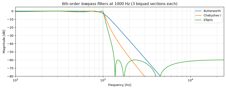
Each row of the SOS matrix is [b0, b1, b2, a0, a1, a2] for one biquad section, where a0 = 1 (normalised form).
# Inspect the SOS matrix
print(f"Butterworth SOS shape: {sos_butter.shape}")
print(f"Number of sections: {sos_butter.shape[0]}\n")
for i, section in enumerate(sos_butter):
    print(f"Section {i+1}: b = [{section[0]:.6f}, {section[1]:.6f}, {section[2]:.6f}]")
    print(f"           a = [{section[3]:.6f}, {section[4]:.6f}, {section[5]:.6f}]")
Butterworth SOS shape: (3, 6)
Number of sections: 3
Section 1: b = [0.000000, 0.000000, 0.000000]
a = [1.000000, -1.760880, 0.776075]
Section 2: b = [1.000000, 2.000000, 1.000000]
a = [1.000000, -1.815341, 0.831006]
Section 3: b = [1.000000, 2.000000, 1.000000]
a = [1.000000, -1.918091, 0.934643]Audio equalizer example
Standard filter design functions produce lowpass/highpass/bandpass filters, but audio equalization requires parametric EQ sections: peaking filters with adjustable gain at a specific frequency, and shelving filters that boost or cut entire frequency bands. These are not directly available in SciPy but can be designed from the Audio EQ Cookbook formulas (Bristow-Johnson 1994).
The key parametric EQ types:
- Low shelf: boost or cut all frequencies below a corner frequency
- Peaking (bell): boost or cut around a center frequency with adjustable bandwidth
- High shelf: boost or cut all frequencies above a corner frequency
def design_peaking_eq(fc, gain_db, Q, fs):
    """Design a peaking EQ biquad section.

    Parameters
    ----------
    fc : float - Center frequency in Hz
    gain_db : float - Gain at center frequency in dB
    Q : float - Quality factor (higher = narrower)
    fs : float - Sample rate in Hz

    Returns
    -------
    sos : ndarray, shape (1, 6) - SOS matrix row
    """
    A = 10**(gain_db / 40)  # amplitude
    w0 = 2 * np.pi * fc / fs
    alpha = np.sin(w0) / (2 * Q)

    b0 = 1 + alpha * A
    b1 = -2 * np.cos(w0)
    b2 = 1 - alpha * A
    a0 = 1 + alpha / A
    a1 = -2 * np.cos(w0)
    a2 = 1 - alpha / A

    return np.array([[b0/a0, b1/a0, b2/a0, 1, a1/a0, a2/a0]])

def design_low_shelf(fc, gain_db, Q, fs):
    """Design a low shelf biquad section."""
    A = 10**(gain_db / 40)
    w0 = 2 * np.pi * fc / fs
    alpha = np.sin(w0) / (2 * Q)

    b0 = A * ((A + 1) - (A - 1)*np.cos(w0) + 2*np.sqrt(A)*alpha)
    b1 = 2*A * ((A - 1) - (A + 1)*np.cos(w0))
    b2 = A * ((A + 1) - (A - 1)*np.cos(w0) - 2*np.sqrt(A)*alpha)
    a0 = (A + 1) + (A - 1)*np.cos(w0) + 2*np.sqrt(A)*alpha
    a1 = -2 * ((A - 1) + (A + 1)*np.cos(w0))
    a2 = (A + 1) + (A - 1)*np.cos(w0) - 2*np.sqrt(A)*alpha

    return np.array([[b0/a0, b1/a0, b2/a0, 1, a1/a0, a2/a0]])

def design_high_shelf(fc, gain_db, Q, fs):
    """Design a high shelf biquad section."""
    A = 10**(gain_db / 40)
    w0 = 2 * np.pi * fc / fs
    alpha = np.sin(w0) / (2 * Q)

    b0 = A * ((A + 1) + (A - 1)*np.cos(w0) + 2*np.sqrt(A)*alpha)
    b1 = -2*A * ((A - 1) + (A + 1)*np.cos(w0))
    b2 = A * ((A + 1) + (A - 1)*np.cos(w0) - 2*np.sqrt(A)*alpha)
    a0 = (A + 1) - (A - 1)*np.cos(w0) + 2*np.sqrt(A)*alpha
    a1 = 2 * ((A - 1) - (A + 1)*np.cos(w0))
    a2 = (A + 1) - (A - 1)*np.cos(w0) - 2*np.sqrt(A)*alpha

    return np.array([[b0/a0, b1/a0, b2/a0, 1, a1/a0, a2/a0]])
fs = 48000
# Design three EQ bands
low_shelf = design_low_shelf(fc=200, gain_db=6, Q=0.707, fs=fs)
peaking = design_peaking_eq(fc=1000, gain_db=-4, Q=2, fs=fs)
high_shelf = design_high_shelf(fc=8000, gain_db=5, Q=0.707, fs=fs)
# Cascade: stack into a single SOS matrix
eq_sos = np.vstack([low_shelf, peaking, high_shelf])
fig, ax = plt.subplots(figsize=(10, 4.5))
# Plot individual bands
for sos, label, color in [(low_shelf, 'Low shelf (+6 dB @ 200 Hz)', 'C0'),
(peaking, 'Peaking (-4 dB @ 1 kHz)', 'C1'),
(high_shelf, 'High shelf (+5 dB @ 8 kHz)', 'C2')]:
w, H = sosfreqz(sos, worN=4096, fs=fs)
ax.semilogx(w[1:], 20*np.log10(np.maximum(np.abs(H[1:]), 1e-10)),
'--', color=color, alpha=0.5, linewidth=1, label=label)
# Plot combined response
w, H = sosfreqz(eq_sos, worN=4096, fs=fs)
ax.semilogx(w[1:], 20*np.log10(np.maximum(np.abs(H[1:]), 1e-10)),
'k-', linewidth=2, label='Combined EQ')
ax.set_xlabel('Frequency [Hz]')
ax.set_ylabel('Gain [dB]')
ax.set_ylim(-10, 12)
ax.set_xlim(20, fs/2)
ax.axhline(0, color='k', linestyle='-', alpha=0.2)
ax.legend(fontsize=8, loc='upper left')
ax.grid(True, alpha=0.3, which='both')
ax.set_title('3-band parametric equalizer')
fig.tight_layout()
plt.show()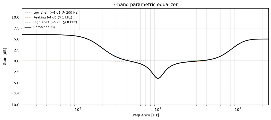
This is the essence of parametric equalization: each band is one biquad, and the cascade of all bands gives the combined EQ curve. Professional audio equalizers use 5 to 31 bands, each independently adjustable, still just a cascade of biquads.
Real-world audio chains
Every audio device you own runs biquads: phone equalizers, hearing aids, studio monitors, car audio DSPs, Bluetooth speakers. A typical audio processing chain is: HPF (remove DC offset and low-frequency rumble, \(f_c \approx 20\)–\(40\) Hz) followed by parametric EQ (3–10 bands of peaking/shelving filters for tonal shaping) followed by a limiter or compressor (often with its own sidechain filter). Each stage is a cascade of biquad sections.
Sample rates in audio range from 44.1 kHz (CD) through 48 kHz (broadcast/video) to 96 or 192 kHz (high-resolution studio work). When the sample rate changes, all biquad coefficients must be recalculated from the underlying frequency/Q/gain parameters, because the coefficients themselves are sample-rate-dependent. This is why audio EQ code stores design parameters (center frequency, bandwidth, gain) rather than raw coefficients, and recomputes on sample rate change.
Implementation considerations
Fixed-point arithmetic
On DSPs without hardware floating-point (or where fixed-point is preferred for power/cost reasons), biquad coefficients and state variables must be represented in fixed-point, typically Q15 (16-bit) or Q31 (32-bit) format.
The critical issue is coefficient quantization. With Q15 format, coefficients are quantized to a grid of \(2^{-15} \approx 3 \times 10^{-5}\). For a narrowband filter with poles close to the unit circle, this grid may be too coarse to place the poles accurately, causing the actual filter response to deviate significantly from the design.
fs = 8000
fc = 1000

# Design a narrow bandpass using a peaking filter
sos_float = design_peaking_eq(fc=fc, gain_db=12, Q=20, fs=fs)

def quantize_sos(sos, bits):
    """Quantize SOS coefficients to fixed-point with clipping."""
    scale = 2**(bits - 1)
    max_val = (scale - 1) / scale  # e.g. 0.999969 for Q15
    sos_q = sos.copy()
    # Don't quantize the '1' in a[0]
    for col in [0, 1, 2, 4, 5]:
        sos_q[:, col] = np.round(sos[:, col] * scale) / scale
        sos_q[:, col] = np.clip(sos_q[:, col], -1.0, max_val)
    return sos_q

sos_q16 = quantize_sos(sos_float, 16)
sos_q32 = quantize_sos(sos_float, 32)

fig, ax = plt.subplots(figsize=(10, 4))
for sos, label, ls, lw in [(sos_float, 'Float64', '-', 2),
                             (sos_q32, 'Q31 (32-bit)', '--', 1.5),
                             (sos_q16, 'Q15 (16-bit)', ':', 1.5)]:
    w, H = sosfreqz(sos, worN=4096, fs=fs)
    ax.plot(w, 20*np.log10(np.maximum(np.abs(H), 1e-10)),
            linestyle=ls, linewidth=lw, label=label)

ax.set_xlabel('Frequency [Hz]')
ax.set_ylabel('Magnitude [dB]')
ax.set_xlim(500, 1500)
ax.legend(fontsize=9)
ax.grid(True, alpha=0.3)
ax.set_title(f'Coefficient quantization: peaking filter at {fc} Hz (Q=20)')
fig.tight_layout()
plt.show()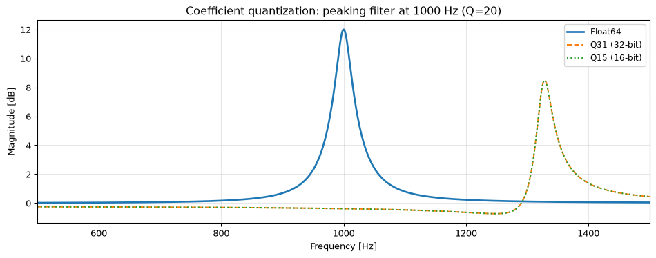
Coefficients greater than 1
In Q15 format, representable values lie in \([-1, 1)\). Filter designs with high gain or sharp resonances can produce coefficients with \(|b_k| > 1\). The quantize_sos function above clips these to the representable range, which distorts the filter response. The practical remedy is gain staging: scale the numerator coefficients of each section so that all \(|b_k| \le 1\), and compensate by distributing the excess gain to other sections or applying it as a separate output gain stage.
Double-precision accumulator
Even with 16-bit coefficients and data, the multiply-accumulate operations in the difference equation should use a wider accumulator, typically 32 or 40 bits. Without this, rounding errors accumulate within each sample computation and can cause limit cycles (small persistent oscillations at the output even when the input is zero).
Most DSP architectures (ARM Cortex-M4, TI C5x/C6x, Analog Devices SHARC) provide 32-bit or 40-bit accumulators specifically for this purpose. ARM’s CMSIS-DSP library offers both arm_biquad_cascade_df1_q15 (with 64-bit accumulator) and arm_biquad_cascade_df1_f32 variants.
Gain scaling
When cascading multiple biquad sections, the signal level at each intermediate stage matters. If a section has gain greater than 0 dB at any frequency, the signal can clip before reaching the next section, even if the overall filter has unity gain. Proper gain distribution across sections (scaling the \(b_0\) coefficients) prevents internal overflow.
For an in-depth treatment of biquad implementation on microcontrollers, see Biquad on Hardware.
Open questions
Coefficient interpolation. When filter parameters change in real time (e.g., a user turning an EQ knob, or an adaptive system updating biquad parameters), naively swapping coefficients between samples can produce clicks and transients. The standard workaround is to interpolate coefficients linearly over a short crossfade window (typically 5–10 ms). But linear interpolation of biquad coefficients does not correspond to linear interpolation of the frequency response, and the intermediate states during the crossfade may have unexpected resonance peaks. Interpolating in the pole-zero domain or using parameter smoothing in the frequency/Q/gain space are alternatives, but neither is fully satisfactory. This remains an area of active work in audio plugin development.
Time-varying biquads. Closely related: when biquad coefficients change continuously (e.g., an auto-wah effect or a tracking filter), the filter is no longer LTI and standard frequency-domain analysis does not strictly apply. The system can exhibit behaviors not predicted by the instantaneous transfer function, including instability if poles cross the unit circle during transitions. Analysis frameworks for linear time-varying (LTV) systems exist but are considerably more complex than the LTI theory covered here.
Numerical equivalence across platforms. The same biquad coefficients processed with IEEE 754 single-precision can give slightly different outputs on different hardware due to fused multiply-add (FMA) instructions, different rounding modes, and compiler optimization levels. For applications requiring bit-exact reproducibility across platforms (e.g., codec standardization), fixed-point with explicit rounding is preferred, but this adds implementation complexity.
References
Bristow-Johnson, Robert. 1994. “Cookbook Formulae for Audio EQ Biquad Filter Coefficients.” https://www.w3.org/2011/audio/audio-eq-cookbook.html.
Robles, Luis, and Mario A. Ruggero. 2001. “Mechanics of the Mammalian Cochlea.” Physiological Reviews 81 (3): 1305–52.