PSD estimation measures what is there. This page is the synthesis counterpart: how to build noise with exactly the distribution, spectrum, and spatial structure you need. Whether you are simulating a sensor for testing, generating a procedural texture, or creating controlled-noise test signals for an ADC characterisation, you need noise you can trust, and verifying that trust means knowing how the generator works.
The companion module noise_generation.py implements every method from first principles.
The Box-Muller transform (Box and Muller 1958) converts two independent uniform(0,1) variates \(u_1, u_2\) into two independent standard normal variates:
It is exact, simple, and sufficient for the vast majority of DSP work. The Ziggurat algorithm (Marsaglia and Tsang 2000) is faster for large \(N\) and ships in NumPy’s default RNG: it partitions the Gaussian PDF into horizontal strips and accepts the vast majority of samples with a single cheap rectangular test, but Box-Muller is what you should implement when you need a generator you understand end-to-end.
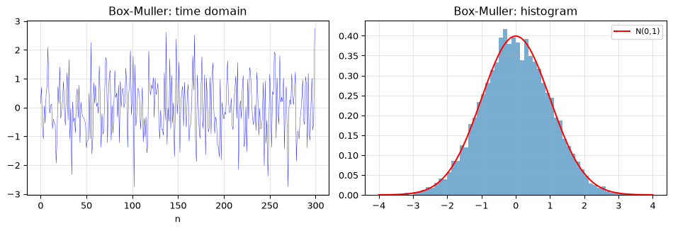
Figure 1: Box-Muller Gaussian noise: 10,000 samples vs the theoretical N(0,1) PDF.
Coloured noise: AR filtering and frequency-domain shaping
AR(p) filtering. The Kasdin recurrence (Kasdin 1995) gives the coefficients of an all-pole filter that turns white noise into \(1/f^\alpha\) noise. For a given exponent \(\alpha\) and model order \(p\), the coefficients are:
The filter \(H(z) = 1 / (1 + \sum_{i=1}^p \theta_i z^{-i})\) shapes the spectrum. Higher \(p\) gives a better fit at low frequencies.
Frequency-domain shaping. Multiply the spectrum of white noise by \(f^{-\alpha/2}\) and inverse-FFT. Simpler but produces a periodic sequence (the last sample wraps to the first).
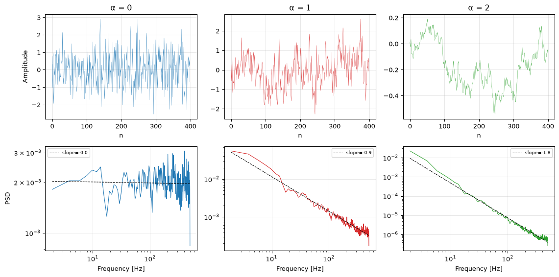
Figure 2: 1/f^alpha noise for alpha = 0 (white), 1 (pink), and 2 (brown). Top: time domain. Bottom: PSD with fitted slope.
Voss-McCartney: pink noise with integer arithmetic
The Voss-McCartney algorithm (Voss’s octave-update scheme from the original \(1/f\)-music study (Voss and Clarke 1978), as refined by McCartney) generates approximate \(1/f\) noise by summing independent white noise generators running at octave-spaced update rates. One generator updates every sample, one every 2 samples, one every 4, and so on; their sum approximates a \(1/f\) spectrum. The algorithm runs in O(\(n\)) time with O(octaves) state and uses only addition: no FFT, no filter, no floating-point multiplies. This makes it uniquely suited to embedded systems.
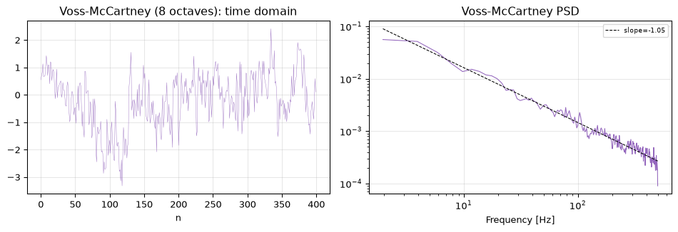
Figure 3: Voss-McCartney pink noise: time domain and PSD. 8 octaves gives a reasonable 1/f approximation with integer-friendly arithmetic.
Perlin noise: noise as a designed signal
Perlin noise Perlin (2002) is not a random process in the stochastic sense. It is a deterministic, procedurally-generated, band-limited noise field: given the same input coordinates, it always produces the same output. The randomness is in a permutation table (a seeded hash), not in the sampling. This makes it fundamentally different from every other noise type on this page: you design its spectral properties by construction rather than filtering.
How it works
Lattice + gradient vectors. Define an integer lattice. At each lattice point, assign a random unit-length gradient vector via a hash of the lattice coordinates.
Dot products. For a query point, find the surrounding lattice cell. Compute the dot product of each corner’s gradient vector with the offset from that corner to the query point.
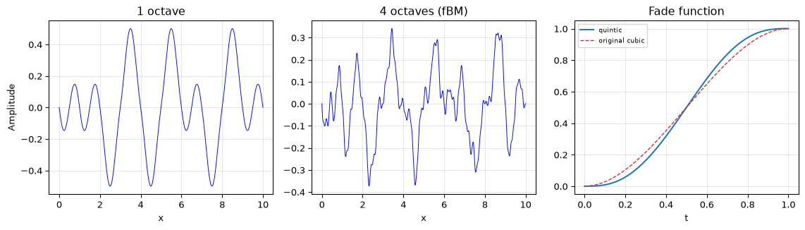
Fade function. Interpolate the corner dot products using a smooth kernel. Perlin’s original fade \(3t^2 - 2t^3\) was replaced in 2002 by the quintic \(6t^5 - 15t^4 + 10t^3\), which has continuous first and second derivatives at lattice boundaries, eliminating the faint directional artifact visible in the second derivative of the original kernel.
Octave summation. Sum scaled copies at doubled frequencies: each octave has twice the spatial frequency and persistence times the amplitude. This builds a \(1/f\)-like spectrum by construction, not by filtering.
The DSP insight: the lattice spacing is a hard low-pass filter. No frequency above the Nyquist of the lattice grid can appear. Perlin noise is band-limited by construction, unlike filtered white noise, which always leaks some energy.
Figure 4: Perlin noise construction. Left: single-octave base Perlin (smooth, low-frequency). Center: four octaves of fractal Brownian motion (rich detail). Right: the quintic fade function (the interpolation kernel that determines the spectral roll-off).
2-D Perlin noise
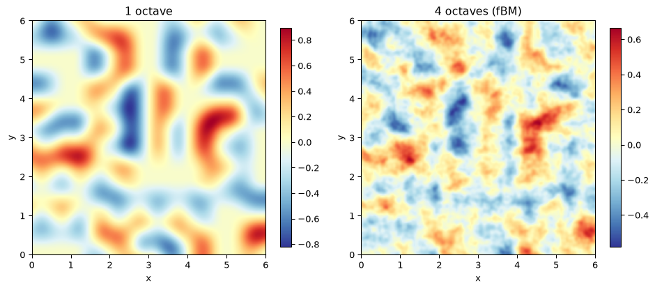
In two dimensions the same construction applies, with four corner gradients per lattice cell and bilinear interpolation in the faded coordinates. Octave-summed 2-D Perlin is the classic procedural texture: terrain heightmaps, cloud patterns, marble veins, and it teaches the spatial-frequency intuition directly.
Figure 5: 2-D Perlin noise. Left: single octave (one spatial scale). Right: four octaves (fractal Brownian motion): note the rich multi-scale detail.
Simplex noise: fewer artifacts, lower complexity
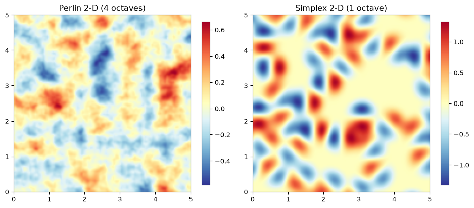
Simplex noise addresses two Perlin limitations: directional artifacts (the square lattice produces visible axis alignment) and computational complexity (\(O(2^D)\) for \(D\)-dimensional Perlin vs \(O(D^2)\) for Simplex). In 2-D, the square lattice is replaced by a triangular (simplex) grid; each point is influenced by only three gradient vectors instead of four.
Figure 6: Simplex vs Perlin noise at the same scale. Simplex shows less visible axis alignment: the triangular grid breaks the directional bias of the square Perlin lattice.
Verification: closing the loop
You generate noise to a specification. PSD estimation verifies that you got what you asked for. The verify_noise() function prints the key diagnostics: distribution moments, ACF, PSD slope, so you can confirm that your pink noise is actually pink and your Perlin field has the expected spatial spectrum.
Generating controlled-noise test signals on a microcontroller, or a procedural terrain for an embedded display, is covered in the embedded companion, including Perlin on integer arithmetic and the Voss-McCartney algorithm’s natural fit for MCUs with no FPU.
Going further
Random processes: the process classes whose outputs you are simulating.
PSD estimation: the measurement side: verify that your generated noise matches its specification.
Noise whitening: the analysis counterpart, whitening removes the correlation that generation adds.
Dither: one of the few DSP applications where you deliberately add noise, and you need a trusted generator to do it right.
References
Box, George E. P., and Mervin E. Muller. 1958. “A Note on the Generation of Random Normal Deviates.”The Annals of Mathematical Statistics 29 (2): 610–11.
Kasdin, N. Jeremy. 1995. “Discrete Simulation of Colored Noise and Stochastic Processes and 1/f^α Power Law Noise Generation.”Proceedings of the IEEE 83 (5): 802–27. https://doi.org/10.1109/5.381848.
Marsaglia, George, and Wai Wan Tsang. 2000. “The Ziggurat Method for Generating Random Variables.”Journal of Statistical Software 5 (8): 1–7.
———. 2002. “Improving Noise.” In Proceedings of the 29th Annual Conference on Computer Graphics and Interactive Techniques (SIGGRAPH 2002), 681–82.
Voss, Richard F., and John Clarke. 1978. “‘1/f Noise’ in Music: Music from 1/f Noise.”Journal of the Acoustical Society of America 63 (1): 258–63.
Source Code
---title: "Noise Generation"subtitle: "Building noise with the properties you specify"description-meta: "Building noise with the distribution, spectrum and spatial structure you specify, for sensor simulation, test injection and procedural texture."bibliography: ../../references.bib---[PSD estimation](../psd-estimation/index.qmd) measures what is there. This page is the synthesis counterpart: how to *build* noise with exactly the distribution, spectrum, and spatial structure you need. Whether you are simulating a sensor for testing, generating a procedural texture, or creating controlled-noise test signals for an ADC characterisation, you need noise you can trust, and verifying that trust means knowing how the generator works.The companion module `noise_generation.py` implements every method from first principles.::: {.callout-note title="Prerequisites"}Part of the [noise & stochastic processing arc](../noise-and-stochastic-processing.qmd); the overview gives the reading order.[Noise and SNR](../../basics/03-noise-snr.qmd) (distributions, white vs coloured), [random processes](../random-processes/index.qmd) (the process classes you are simulating), and [PSD estimation](../psd-estimation/index.qmd) (how to verify the output).:::::: {.callout-tip title="Code"}The implementation is [`noise_generation.py`](noise_generation.py). Save [`test_noise_generation.py`](test_noise_generation.py) beside it and `pytest test_noise_generation.py` runs the checks on it.:::```{python}#| echo: falseimport numpy as npimport matplotlib.pyplot as pltfrom noise_generation import (box_muller, ziggurat, colored_noise_ar, colored_noise_fd, voss_mccartney, perlin_1d, perlin_2d, simplex_2d, verify_noise)```<hr>## Gaussian generation: Box-MullerThe Box-Muller transform [@box1958note] converts two independent uniform(0,1) variates $u_1, u_2$ into two independent standard normal variates:$$z_0 = \sqrt{-2\ln u_1}\,\cos(2\pi u_2), \qquad z_1 = \sqrt{-2\ln u_1}\,\sin(2\pi u_2)$$It is exact, simple, and sufficient for the vast majority of DSP work. The Ziggurat algorithm [@marsaglia2000ziggurat] is faster for large $N$ and ships in NumPy's default RNG: it partitions the Gaussian PDF into horizontal strips and accepts the vast majority of samples with a single cheap rectangular test, but Box-Muller is what you should implement when you need a generator you understand end-to-end.```{python}#| label: fig-box-muller#| fig-cap: "Box-Muller Gaussian noise: 10,000 samples vs the theoretical N(0,1) PDF."x = box_muller(10000, seed=42)fig, axes = plt.subplots(1, 2, figsize=(10, 3.5))axes[0].plot(x[:300], 'b-', linewidth=0.3)axes[0].set_title('Box-Muller: time domain'); axes[0].set_xlabel('n'); axes[0].grid(True, alpha=0.3)axes[1].hist(x, bins=60, density=True, alpha=0.6, color='C0')xr = np.linspace(-4, 4, 200)axes[1].plot(xr, np.exp(-xr**2/2)/np.sqrt(2*np.pi), 'r-', linewidth=1.5, label='N(0,1)')axes[1].set_title('Box-Muller: histogram'); axes[1].legend(fontsize=8); axes[1].grid(True, alpha=0.3)fig.tight_layout(); plt.show()assertabs(np.mean(x)) <0.05and0.95< np.std(x) <1.05, "Should be N(0,1)"```<hr>## Coloured noise: AR filtering and frequency-domain shaping**AR(p) filtering.** The Kasdin recurrence [@kasdin1995discrete] gives the coefficients of an all-pole filter that turns white noise into $1/f^\alpha$ noise. For a given exponent $\alpha$ and model order $p$, the coefficients are:$$\theta_i = \frac{(i - 1 - \alpha/2) \cdot \theta_{i-1}}{i}, \quad \theta_0 = 1$$The filter $H(z) = 1 / (1 + \sum_{i=1}^p \theta_i z^{-i})$ shapes the spectrum. Higher $p$ gives a better fit at low frequencies.**Frequency-domain shaping.** Multiply the spectrum of white noise by $f^{-\alpha/2}$ and inverse-FFT. Simpler but produces a periodic sequence (the last sample wraps to the first).```{python}#| label: fig-colored-noise#| fig-cap: "1/f^alpha noise for alpha = 0 (white), 1 (pink), and 2 (brown). Top: time domain. Bottom: PSD with fitted slope."from scipy.signal import welchalphas = [0.0, 1.0, 2.0]colors = ['C0', 'C3', 'C2']n =10000fs =1000fig, axes = plt.subplots(2, 3, figsize=(12, 6))for j, alpha inenumerate(alphas): x = colored_noise_ar(n, alpha=alpha, p=30, seed=42) axes[0, j].plot(x[:400], color=colors[j], linewidth=0.3) axes[0, j].set_title(f'α = {alpha:.0f}') axes[0, j].set_xlabel('n'); axes[0, j].grid(True, alpha=0.3) f, psd = welch(x, fs, nperseg=512) axes[1, j].loglog(f[1:], psd[1:], color=colors[j], linewidth=0.8)# Fit slope mask = f >0 coeffs = np.polyfit(np.log10(f[mask]), np.log10(psd[mask]), 1)# The caption's claim is the fitted exponent itself: -alpha within 0.2# (measured: -0.006 / -0.915 / -1.818 for alpha = 0 / 1 / 2).assertabs(coeffs[0] - (-alpha)) <0.2, \f"alpha={alpha}: fitted slope {coeffs[0]:.2f}, expected ~{-alpha}" axes[1, j].loglog(f[1:], 10**coeffs[1] * f[1:]**coeffs[0], 'k--', linewidth=0.8, label=f'slope={coeffs[0]:.1f}') axes[1, j].set_xlabel('Frequency [Hz]'); axes[1, j].legend(fontsize=7); axes[1, j].grid(True, alpha=0.3)axes[0, 0].set_ylabel('Amplitude'); axes[1, 0].set_ylabel('PSD')fig.tight_layout(); plt.show()```<hr>## Voss-McCartney: pink noise with integer arithmeticThe Voss-McCartney algorithm (Voss's octave-update scheme from the original $1/f$-music study [@voss1978noise], as refined by McCartney) generates approximate $1/f$ noise by summing independent white noise generators running at octave-spaced update rates. One generator updates every sample, one every 2 samples, one every 4, and so on; their sum approximates a $1/f$ spectrum. The algorithm runs in O($n$) time with O(octaves) state and uses only addition: no FFT, no filter, no floating-point multiplies. This makes it uniquely suited to embedded systems.```{python}#| label: fig-voss-mccartney#| fig-cap: "Voss-McCartney pink noise: time domain and PSD. 8 octaves gives a reasonable 1/f approximation with integer-friendly arithmetic."x = voss_mccartney(10000, octaves=8, seed=42)fig, axes = plt.subplots(1, 2, figsize=(10, 3.5))axes[0].plot(x[:400], 'C4-', linewidth=0.3)axes[0].set_title('Voss-McCartney (8 octaves): time domain')axes[0].set_xlabel('n'); axes[0].grid(True, alpha=0.3)f, psd = welch(x, 1000, nperseg=512)axes[1].loglog(f[1:], psd[1:], 'C4-', linewidth=0.8)coeffs = np.polyfit(np.log10(f[1:]), np.log10(psd[1:]), 1)# "A reasonable 1/f approximation" = fitted slope near -1 (measured -1.05).assert-1.3< coeffs[0] <-0.7, f"expected ~1/f (slope -1), got {coeffs[0]:.2f}"axes[1].loglog(f[1:], 10**coeffs[1] * f[1:]**coeffs[0], 'k--', linewidth=0.8, label=f'slope={coeffs[0]:.2f}')axes[1].set_title('Voss-McCartney PSD'); axes[1].set_xlabel('Frequency [Hz]')axes[1].legend(fontsize=7); axes[1].grid(True, alpha=0.3)fig.tight_layout(); plt.show()```<hr>## Perlin noise: noise as a designed signalPerlin noise [@perlin1985image, @perlin2002improving] is not a random process in the stochastic sense. It is a **deterministic, procedurally-generated, band-limited noise field**: given the same input coordinates, it always produces the same output. The randomness is in a permutation table (a seeded hash), not in the sampling. This makes it fundamentally different from every other noise type on this page: you design its spectral properties by construction rather than filtering.### How it works1. **Lattice + gradient vectors.** Define an integer lattice. At each lattice point, assign a random unit-length gradient vector via a hash of the lattice coordinates.2. **Dot products.** For a query point, find the surrounding lattice cell. Compute the dot product of each corner's gradient vector with the offset from that corner to the query point.3. **Fade function.** Interpolate the corner dot products using a smooth kernel. Perlin's original fade $3t^2 - 2t^3$ was replaced in 2002 by the quintic $6t^5 - 15t^4 + 10t^3$, which has continuous first and second derivatives at lattice boundaries, eliminating the faint directional artifact visible in the second derivative of the original kernel.4. **Octave summation.** Sum scaled copies at doubled frequencies: each octave has twice the spatial frequency and `persistence` times the amplitude. This builds a $1/f$-like spectrum by construction, not by filtering.The DSP insight: **the lattice spacing is a hard low-pass filter**. No frequency above the Nyquist of the lattice grid can appear. Perlin noise is band-limited by construction, unlike filtered white noise, which always leaks some energy.```{python}#| label: fig-perlin-construction#| fig-cap: "Perlin noise construction. Left: single-octave base Perlin (smooth, low-frequency). Center: four octaves of fractal Brownian motion (rich detail). Right: the quintic fade function (the interpolation kernel that determines the spectral roll-off)."x = np.linspace(0, 10, 1000)fig, axes = plt.subplots(1, 3, figsize=(12, 3.5))y1 = perlin_1d(x, seed=1, octaves=1)axes[0].plot(x, y1, 'b-', linewidth=0.7)axes[0].set_title('1 octave'); axes[0].set_xlabel('x'); axes[0].set_ylabel('Amplitude')axes[0].grid(True, alpha=0.3)y4 = perlin_1d(x, seed=1, octaves=4, persistence=0.5)axes[1].plot(x, y4, 'b-', linewidth=0.7)axes[1].set_title('4 octaves (fBM)'); axes[1].set_xlabel('x')axes[1].grid(True, alpha=0.3)# Fade functiont = np.linspace(0, 1, 200)fade_old =3*t**2-2*t**3fade_quintic =6*t**5-15*t**4+10*t**3axes[2].plot(t, fade_quintic, 'C0-', linewidth=1.5, label='quintic')axes[2].plot(t, fade_old, 'C3--', linewidth=1, label='original cubic')axes[2].set_title('Fade function'); axes[2].set_xlabel('t'); axes[2].legend(fontsize=7)axes[2].grid(True, alpha=0.3)fig.tight_layout(); plt.show()# Verify: single-octave Perlin is zero at integer lattice points.test_x = np.array([0.0, 1.0, 2.0, 3.0])y_zero = perlin_1d(test_x, seed=0, octaves=1)assert np.allclose(y_zero, 0.0, atol=1e-10), "Single-octave Perlin should be zero at integer lattice points"```### 2-D Perlin noiseIn two dimensions the same construction applies, with four corner gradients per lattice cell and bilinear interpolation in the faded coordinates. Octave-summed 2-D Perlin is the classic procedural texture: terrain heightmaps, cloud patterns, marble veins, and it teaches the spatial-frequency intuition directly.```{python}#| label: fig-perlin-2d#| fig-cap: "2-D Perlin noise. Left: single octave (one spatial scale). Right: four octaves (fractal Brownian motion): note the rich multi-scale detail."size =200X, Y = np.meshgrid(np.linspace(0, 6, size), np.linspace(0, 6, size), indexing='ij')fig, axes = plt.subplots(1, 2, figsize=(10, 4.5))for ax, octaves, title inzip(axes, [1, 4], ['1 octave', '4 octaves (fBM)']): Z = perlin_2d(X, Y, seed=42, octaves=octaves, persistence=0.5) im = ax.imshow(Z.T, origin='lower', cmap='RdYlBu_r', extent=[0, 6, 0, 6]) ax.set_title(title); ax.set_xlabel('x'); ax.set_ylabel('y') plt.colorbar(im, ax=ax, shrink=0.8)fig.tight_layout(); plt.show()```### Simplex noise: fewer artifacts, lower complexitySimplex noise addresses two Perlin limitations: directional artifacts (the square lattice produces visible axis alignment) and computational complexity ($O(2^D)$ for $D$-dimensional Perlin vs $O(D^2)$ for Simplex). In 2-D, the square lattice is replaced by a triangular (simplex) grid; each point is influenced by only three gradient vectors instead of four.```{python}#| label: fig-simplex-vs-perlin#| fig-cap: "Simplex vs Perlin noise at the same scale. Simplex shows less visible axis alignment: the triangular grid breaks the directional bias of the square Perlin lattice."size =150X, Y = np.meshgrid(np.linspace(0, 5, size), np.linspace(0, 5, size), indexing='ij')fig, axes = plt.subplots(1, 2, figsize=(10, 4.5))Z_perlin = perlin_2d(X, Y, seed=42, octaves=4, persistence=0.5)im0 = axes[0].imshow(Z_perlin.T, origin='lower', cmap='RdYlBu_r', extent=[0, 5, 0, 5])axes[0].set_title('Perlin 2-D (4 octaves)'); plt.colorbar(im0, ax=axes[0], shrink=0.8)Z_simplex = simplex_2d(X, Y, seed=42)im1 = axes[1].imshow(Z_simplex.T, origin='lower', cmap='RdYlBu_r', extent=[0, 5, 0, 5])axes[1].set_title('Simplex 2-D (1 octave)'); plt.colorbar(im1, ax=axes[1], shrink=0.8)fig.tight_layout(); plt.show()```<hr>## Verification: closing the loopYou generate noise to a specification. PSD estimation verifies that you got what you asked for. The `verify_noise()` function prints the key diagnostics: distribution moments, ACF, PSD slope, so you can confirm that your pink noise is actually pink and your Perlin field has the expected spatial spectrum.```{python}#| label: fig-verifyfor label, x_gen in [('Pink (AR, p=20)', colored_noise_ar(10000, alpha=1.0, p=20, seed=1)), ('Voss-McCartney', voss_mccartney(10000, octaves=8, seed=1)), ('Perlin 1-D (4 oct)', perlin_1d(np.linspace(0, 50, 2000), seed=1, octaves=4))]: verify_noise(x_gen, label=label)```<hr>## On hardwareGenerating controlled-noise test signals on a microcontroller, or a procedural terrain for an embedded display, is covered in the [embedded companion](embedded.qmd), including Perlin on integer arithmetic and the Voss-McCartney algorithm's natural fit for MCUs with no FPU.<hr>## Going further- **[Random processes](../random-processes/index.qmd)**: the process classes whose outputs you are simulating.- **[PSD estimation](../psd-estimation/index.qmd)**: the measurement side: verify that your generated noise matches its specification.- **[Noise whitening](../noise-whitening/index.qmd)**: the analysis counterpart, whitening removes the correlation that generation adds.- **[Dither](../dither/index.qmd)**: one of the few DSP applications where you deliberately add noise, and you need a trusted generator to do it right.## References::: {#refs}:::