You have a noise record: a sequence of samples from an ADC, a sensor, a simulation. You want to know how its power is distributed across frequency: is it white, pink, brown, or something stranger? Is there a hidden tone buried in the noise? Is the noise floor flat enough for your detection algorithm?
The power spectral density (PSD) answers these questions. Estimating it from a finite record is one of the most practiced operations in DSP, and one of the most misunderstood. The naive approach (square the DFT magnitude) gives an answer, but it is an inconsistent estimator: its variance does not decrease no matter how many samples you collect.
This page walks through the classical methods: the periodogram (and why it is broken), Bartlett’s averaging fix, and Welch’s overlapping-window method that has been the standard since 1967. The companion module psd_estimation.py implements each from first principles.
Noise and SNR (autocorrelation, power, white vs coloured noise), the frequency domain (DFT, spectral leakage, window functions), and random processes (the process classes whose PSDs you are estimating).
The basics chapter defines the autocorrelation \(R_{xx}[k] = E[x[n]\,x[n+k]]\) and notes that for white noise, \(R_{xx}[k] = \sigma^2 \delta[k]\). The Wiener-Khinchin theorem(Proakis and Manolakis 2007) closes the loop: for a wide-sense stationary process, the power spectral density is the Fourier transform of the autocorrelation:
\[S_{xx}(f) = \sum_{k=-\infty}^{\infty} R_{xx}[k]\, e^{-j2\pi f k}\]
and conversely \(R_{xx}[k]\) is the inverse Fourier transform of \(S_{xx}(f)\). This is not just a neat identity; it is the reason the PSD exists as a well-defined quantity for random processes whose individual sample functions may not even have Fourier transforms in the ordinary sense. It is also what licenses every estimator on this page: carrying the same calculation through for a finite record shows that \(E[|X[k]|^2]/N\) converges to this Fourier transform of the autocorrelation, so squaring a DFT really does estimate a PSD. The maximum-likelihood section below builds on exactly that link.
White noise has \(R_{xx}[k] = \sigma^2\delta[k]\), so \(S_{xx}(f) = \sigma^2\): flat. An AR(1) process with \(R_{xx}[k] = \phi^{|k|}\sigma^2\) has a PSD that rolls off as \(1/|1 - \phi e^{-j2\pi f}|^2\). The ACF tells you what to expect; the PSD estimate tells you whether the data matches.
The periodogram, and why it is broken
The simplest estimator: take the DFT of \(N\) samples, square the magnitude. This is the periodogram(Proakis and Manolakis 2007):
where \(X[k] = \sum_{n=0}^{N-1} x[n] e^{-j2\pi kn/N}\). For a one-sided spectrum the interior bins are doubled.
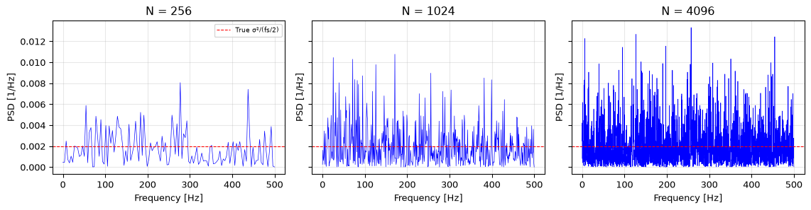
The periodogram is asymptotically unbiased: as \(N \to \infty\), its expected value approaches the true PSD. But it is inconsistent: its variance does not decrease with \(N\). Collect 1000 samples or 100,000; the periodogram is equally jumpy. The variance stays at roughly the square of the PSD value regardless of record length.
The reason: a DFT of length \(N\) has \(N/2+1\) frequency bins. Doubling \(N\) doubles the number of bins but does not improve the estimate at each bin: you are estimating more points, not the same points better. This is the fundamental insight that motivates averaging methods.
Show the code
rng = np.random.default_rng(42)lengths = [256, 1024, 4096]fs =1000fig, axes = plt.subplots(1, 3, figsize=(12, 3.2), sharey=True)for ax, N inzip(axes, lengths): x = rng.standard_normal(N) f, psd = periodogram(x, fs=fs, window='boxcar') ax.plot(f, psd, 'b-', linewidth=0.5) ax.axhline(1/(fs/2), color='r', linestyle='--', linewidth=0.8, label='True σ²/(fs/2)') ax.set_title(f'N = {N}') ax.set_xlabel('Frequency [Hz]'); ax.set_ylabel('PSD [1/Hz]') ax.grid(True, alpha=0.3)if N ==256: ax.legend(fontsize=7)fig.tight_layout(); plt.show()# Verify: the variance of the periodogram ordinates is roughly constant# (equal to squared PSD value for a white noise input).ratios = []for N in lengths: x = rng.standard_normal(N) _, psd = periodogram(x, fs=fs, window='boxcar') var_psd = np.var(psd[1:-1]) # exclude DC mean_psd = np.mean(psd[1:-1]) ratios.append(var_psd / mean_psd**2)print(f"N={N:5d}: var(PSD)={var_psd:.4f}, mean(PSD)²={mean_psd**2:.4f}, ratio={var_psd/mean_psd**2:.2f}")# The caption's claim: the jitter is equally severe at every N. For a# consistent estimator the ratio would fall like 1/N (16x from 256 to 4096);# here it must stay ~1 at every N.for N, r inzip(lengths, ratios):assert0.7< r <1.4, f"N={N}: var/mean^2 = {r:.2f}, expected ~1 (inconsistency)"assertmax(ratios) /min(ratios) <1.3, "ratio should not shrink with N"
Figure 1: The periodogram is inconsistent: variance does not decrease with record length. Each panel shows the periodogram of white noise of increasing length: the jitter is equally severe in all three.
The ratio \(\text{var}(\hat{S}) / E[\hat{S}]^2 \approx 1\) regardless of \(N\): the hallmark of an inconsistent estimator.
Bartlett’s method: average non-overlapping segments
If one long periodogram is jumpy, average several short ones. Bartlett’s method(Proakis and Manolakis 2007) divides the \(N\)-sample record into \(K\) non-overlapping segments of length \(L\), computes the periodogram of each, and averages:
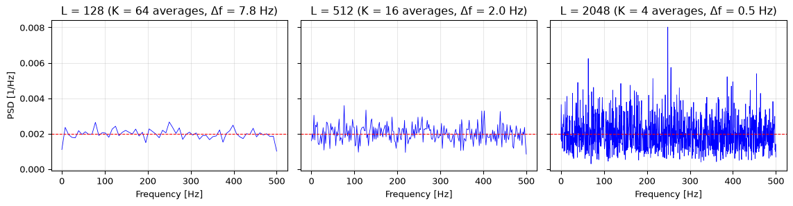
The variance is reduced by a factor of \(K\): you get a smoother estimate. The cost is frequency resolution: each segment is only \(L\) samples long, so the bin spacing is \(f_s/L\) instead of \(f_s/N\). This is the bias-variance trade-off that defines all PSD estimation.
Figure 2: Bartlett’s method: averaging K non-overlapping periodograms. More averages = lower variance but coarser frequency resolution.
With \(K = 64\) segments (\(L = 128\)), the variance is roughly \(1/64\) of a single periodogram, but the frequency resolution is only \(1000/128 \approx 7.8\) Hz, too coarse for many applications.
Why the periodogram? It is (almost) maximum likelihood
This section uses the estimation vocabulary (likelihood, Fisher information, the Cramér-Rao bound) that estimation basics sets up. It is readable without that page, but easier with it.
Everything so far has justified the recipe (square the DFT, average segments) by its behaviour. There is a deeper justification. Under two assumptions (the noise is Gaussian, and its correlation is short compared with the segment length), Bartlett’s procedure is not merely sensible: it is the maximum likelihood estimator of the power in each frequency bin, and its variance achieves the Cramér-Rao lower bound exactly (Kay 1993).
To keep the algebra clean we work with the discrete-time PSD sampled at the bin frequencies, \(S[k] = S_{xx}(k/N)\), and drop the \(1/f_s\) density scaling and one-sided doubling used elsewhere on this page; both multiply the estimator and the true value alike.
The DFT nearly whitens Gaussian noise. Collect one segment \(\underline{x} = (x[0], \ldots, x[N-1])\) of a zero-mean WSS Gaussian process. Its covariance matrix has entries \(R_{xx}[a-b]\): a Toeplitz matrix, constant along diagonals. If the correlation dies out quickly relative to \(N\), a Toeplitz matrix is well approximated by a circulant one, and every circulant matrix is diagonalised by the DFT, with eigenvalues that approach the sampled PSD (Gray 1972). Two consequences follow:
The DFT coefficients \(X[k]\) are nearly uncorrelated across bins, and since they are jointly Gaussian, nearly independent: the DFT acts as an approximate whitener for stationary Gaussian noise.
The variance of each coefficient is the PSD sampled at that bin: \[E\left[|X[k]|^2\right] \approx N\, S[k]\]
For the interior bins (\(0 < k < N/2\)), \(X[k]\) is a zero-mean complex Gaussian: its real and imaginary parts are independent with equal variance \(N S[k]/2\). (The DC and Nyquist bins are purely real; they behave differently, and we return to them below.)
The likelihood of one bin. Now run Bartlett’s procedure: split the record into \(K\) segments, giving independent coefficients \(X_1[k], \ldots, X_K[k]\) at each bin. The density of a zero-mean complex Gaussian with variance \(N S[k]\) is
\[p\left(X_j[k];\, S[k]\right) = \frac{1}{\pi N S[k]} \exp\left(-\frac{|X_j[k]|^2}{N S[k]}\right)\]
so the negative log-likelihood of all \(K\) observations of bin \(k\), viewed as a function of the unknown \(S[k]\), is
\[-\ln L(S[k]) = K \ln\left(\pi N S[k]\right) + \frac{1}{N S[k]} \sum_{j=1}^{K} |X_j[k]|^2\]
Setting the derivative with respect to \(S[k]\) to zero:
which is exactly the averaged periodogram: Bartlett’s estimate. For \(K=1\) it is the raw periodogram. The estimator we introduced as “the simplest thing you could do” is what maximum likelihood tells you to do.
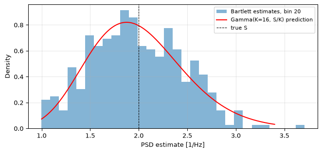
How good is it? Each \(|X_j[k]|^2/N\) is an exponential random variable with mean \(S[k]\) (and hence variance \(S[k]^2\)), so the estimator is unbiased, with
The Fisher information works out to \(I(S[k]) = K/S[k]^2\), so the Cramér-Rao lower bound is \(S[k]^2/K\): the averaged periodogram does not just approach the bound, it sits on it. (Neither property comes free with the ML label: maximum likelihood estimators are only asymptotically unbiased and efficient in general (Kay 1993); here both hold at finite \(K\) because the per-bin model is an exponential family with a linear sufficient statistic.)
This reframes the inconsistency demonstrated at the top of the page. At \(K=1\) the variance equals \(S[k]^2\), and that is the Cramér-Rao bound: the raw periodogram is not a badly designed estimator, it is the best unbiased use of the roughly two degrees of freedom a single segment gives each bin. Lengthening the record buys more bins, not better bins. Averaging is how you spend data on the bins you already have, and the standard deviation falls as \(1/\sqrt{K}\): the same square-root law that governs every averaging operation in this arc.
Two more results drop out of the same per-bin statistics:
\(2|X_j[k]|^2 / (N S[k])\) is \(\chi^2\)-distributed with 2 degrees of freedom, so the sum over \(K\) segments is \(\chi^2_{2K}\): the \(\nu = 2K\) chi-squared model used for the confidence intervals below is this result, not an extra assumption.
Rewriting the ML estimate as a recurrence, \(\hat{S}_K = \frac{K-1}{K}\, \hat{S}_{K-1} + \frac{1}{K} \cdot \frac{|X_K[k]|^2}{N}\), gives a streaming form that needs no segment buffer: this is the accumulate-as-you-go update used on the embedded companion.
The honest caveats: the DC bin (and, for even \(N\), the Nyquist bin) is real rather than complex Gaussian, and its estimator variance is \(2S[k]^2/K\), twice the interior value. The circulant approximation is exact only as \(N \to \infty\); at finite \(N\) its error shows up as the bias and leakage that the windowing discussion already covers. And non-Gaussian noise voids the optimality claim, though the estimator itself remains unbiased whenever the process has a finite second moment.
Show the code
from scipy import statsrng = np.random.default_rng(7)fs =1.0L, K, n_trials =64, 16, 400psds = np.array([bartlett(rng.standard_normal(L * K), fs=fs, nperseg=L, window='boxcar')[1]for _ inrange(n_trials)])interior = psds[:, 1:-1] # drop the real-valued DC/Nyquist binsS_true =2.0/ fs # one-sided density of unit white noisebin_ix =20# an arbitrary interior bin for the histogramfig, ax = plt.subplots(figsize=(7, 3.4))ax.hist(interior[:, bin_ix], bins=30, density=True, alpha=0.55, label=f'Bartlett estimates, bin {bin_ix}')s_grid = np.linspace(0.5* S_true, 1.7* S_true, 300)ax.plot(s_grid, stats.gamma.pdf(s_grid, a=K, scale=S_true / K), 'r-', lw=1.5, label=f'Gamma(K={K}, S/K) prediction')ax.axvline(S_true, color='k', ls='--', lw=0.8, label='true S')ax.set_xlabel('PSD estimate [1/Hz]'); ax.set_ylabel('Density')ax.legend(fontsize=8); ax.grid(True, alpha=0.3)fig.tight_layout(); plt.show()# Verify the ML analysis against the Monte Carlo, bin by bin:mean_ratio = interior.mean(axis=0).mean() / S_truevar_ratio = (interior.var(axis=0) * K / interior.mean(axis=0)**2).mean()print(f"mean/S = {mean_ratio:.3f} (unbiased: expect 1)")print(f"var*K/S^2 = {var_ratio:.3f} (CRLB: expect 1; a real-Gaussian model would give 2)")assert0.98< mean_ratio <1.02, "estimator should be unbiased"assert0.90< var_ratio <1.10, "variance should sit on the CRLB S^2/K"
Figure 3: Sampling distribution of the Bartlett estimate at one interior bin (400 independent records, K = 16 segments of L = 64 samples, unit-variance white Gaussian noise). The histogram matches the Gamma(K, S/K) density predicted by the per-bin ML analysis, and the measured variance sits on the Cramér-Rao bound S²/K rather than the 2S²/K a real-Gaussian model would predict.
mean/S = 0.997  (unbiased: expect 1)
var*K/S^2 = 1.012  (CRLB: expect 1; a real-Gaussian model would give 2)
Welch’s method: overlap to recover lost averages
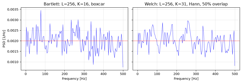
Welch’s method(Welch 1967) improves on Bartlett by allowing segments to overlap. A 50% overlap with a Hann window nearly doubles the number of segments for the same frequency resolution, because the window tapers the segment edges to zero: samples near the boundary contribute little on their own but contribute fully when segments overlap.
The trade-off now involves three knobs:
Knob
What it controls
What you lose
Segment length \(L\)
Frequency resolution \(\Delta f = f_s/L\)
More segments for averaging
Overlap
Number of segments (variance reduction)
Diminishing returns beyond 50% for Hann
Window
Spectral leakage, bias
Hann: low sidelobes; boxcar: best resolution, worst leakage
Figure 4: Welch (50% overlap, Hann) vs Bartlett (no overlap, boxcar) at the same segment length. Welch gives more averages for the same frequency resolution.
Welch with 50% overlap and Hann gives roughly \(2K-1\) effective segments, nearly twice as many as Bartlett at the same frequency resolution.
Comparison against scipy
The module’s welch() matches scipy.signal.welch to within numerical precision when using the same parameters. The implementation is from first principles so you can see every step, but in production you should use scipy’s battle-tested version:
Show the code
rng = np.random.default_rng(99)x = rng.standard_normal(8192)nperseg, noverlap =256, 128f_o, psd_o = welch(x, fs=500, nperseg=nperseg, noverlap=noverlap, window='hann')f_s, psd_s = scipy_welch(x, fs=500, nperseg=nperseg, noverlap=noverlap, window='hann', scaling='density', detrend=False)max_err = np.max(np.abs(psd_o - psd_s) / (psd_s +1e-12))print(f"Max relative error vs scipy: {max_err:.2e}")# "Within numerical precision" is the prose claim, so assert that, not a# loose 5%: float64 round-off is ~1e-16, leave three orders of headroom.assert max_err <1e-12, "Our Welch should match scipy to numerical precision"
Max relative error vs scipy: 9.31e-16
Figure 5
Confidence intervals: how much do you trust that peak?
A PSD estimate without confidence intervals is a line without error bars. The averaged periodogram ordinates are chi-squared distributed with \(\nu = 2K\) degrees of freedom (where \(K\) is the number of averaged segments) (Percival and Walden 1993); this is not an extra modelling assumption but the per-bin statistics derived in the maximum-likelihood section above. A \(100(1-\alpha)\%\) confidence interval for the true PSD at frequency bin \(k\) is
where \(\chi^2_{\nu,q}\) is the \(q\)-quantile of the chi-squared distribution with \(\nu\) degrees of freedom. More averages → narrower intervals → more confidence that a spectral feature is real.
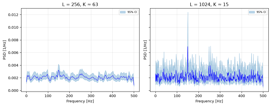
Figure 6: Welch PSD estimate with 95% confidence intervals. Fewer averages = wider intervals. A peak that barely exceeds the interval width is not credible.
The tone at 150 Hz is barely visible in the \(L=256\) estimate: the confidence interval is too wide to distinguish it from a random fluctuation. With \(L=1024\) (fewer averages but finer resolution), the peak narrows and the interval shrinks enough to identify it as a real spectral line.
Practical recipe
Given a noise record x sampled at fs:
Choose \(L\) based on the spectral feature you need to resolve. If you need to separate two tones 10 Hz apart, you need \(\Delta f < 10\) Hz, so \(L > f_s / 10\).
Choose overlap 50% with a Hann window. This is the default for a reason: it gives near-maximum variance reduction with minimal additional correlation between segments.
Check \(K\). If you have fewer than 10 segments, the estimate is noisy and confidence intervals are wide. Collect more data or accept coarser resolution.
Plot with confidence intervals. A feature that does not exceed the interval width is not credible.
Compare against a known reference. White noise at unit variance has PSD \(1/(f_s/2)\). If your estimate differs systematically, check your normalisation.
On hardware
A Welch estimate on a microcontroller requires an FFT, a squared-magnitude accumulation buffer, and the patience to collect enough data. See the embedded companion for a fixed-point implementation on the ESP32-S3 and STM32F4, including the memory budget, the accumulation-in-place trick, and how to verify your estimate against the known quantization noise floor.
Going further
Noise whitening: the PSD slope is the input to the whitening filter: estimate \(\alpha\), build the inverse filter.
ADC noise: PSD estimation on real ADC data reveals jitter, INL/DNL signatures, and the noise floor that the 6.02 formula does not capture.
Estimation basics: the general theory the maximum-likelihood section above is an instance of: bias, variance, consistency, and the Cramér-Rao bound.
Random processes: each process class has a characteristic PSD shape: flat for white, \(1/f^\alpha\) for power-law, Lorentzian for RTS.
Open question: PSD estimation of non-stationary noise
Welch’s method assumes stationarity: the PSD does not change over the record. For non-stationary noise (a sensor warming up, an amplifier whose noise figure drifts with temperature, a cyclostationary process observed over too few periods), a single PSD estimate is misleading. The time-frequency extensions (spectrogram, multitaper spectrogram, wavelet scalogram) are the tools for that case; see the STFT topic as the starting point.
References
Gray, Robert M. 1972. “On the Asymptotic Eigenvalue Distribution of Toeplitz Matrices.”IEEE Transactions on Information Theory 18 (6): 725–30. https://doi.org/10.1109/TIT.1972.1054924.
Kay, Steven M. 1993. Fundamentals of Statistical Signal Processing, Volume i: Estimation Theory. Upper Saddle River, NJ: Prentice Hall.
Percival, Donald B., and Andrew T. Walden. 1993. Spectral Analysis for Physical Applications. Cambridge University Press.
Proakis, John G., and Dimitris G. Manolakis. 2007. Digital Signal Processing: Principles, Algorithms, and Applications. 4th ed. Pearson.
Welch, Peter D. 1967. “The Use of Fast Fourier Transform for the Estimation of Power Spectra: A Method Based on Time Averaging over Short, Modified Periodograms.”IEEE Transactions on Audio and Electroacoustics 15 (2): 70–73.
Source Code
---title: "PSD Estimation"subtitle: "Measuring what you cannot see directly"description-meta: "Measuring how a signal's power is distributed across frequency: the periodogram, Welch's method, windowing, and confidence intervals."bibliography: ../../references.bib---You have a noise record: a sequence of samples from an ADC, a sensor, a simulation. You want to know how its power is distributed across frequency: is it white, pink, brown, or something stranger? Is there a hidden tone buried in the noise? Is the noise floor flat enough for your detection algorithm?The **power spectral density** (PSD) answers these questions. Estimating it from a finite record is one of the most practiced operations in DSP, and one of the most misunderstood. The naive approach (square the DFT magnitude) gives an answer, but it is an *inconsistent* estimator: its variance does not decrease no matter how many samples you collect.This page walks through the classical methods: the periodogram (and why it is broken), Bartlett's averaging fix, and Welch's overlapping-window method that has been the standard since 1967. The companion module `psd_estimation.py` implements each from first principles.::: {.callout-note title="Prerequisites"}Part of the [noise & stochastic processing arc](../noise-and-stochastic-processing.qmd); the overview gives the reading order.[Noise and SNR](../../basics/03-noise-snr.qmd) (autocorrelation, power, white vs coloured noise), [the frequency domain](../../basics/05-frequency-domain.qmd) (DFT, spectral leakage, window functions), and [random processes](../random-processes/index.qmd) (the process classes whose PSDs you are estimating).:::::: {.callout-tip title="Code"}The implementation is [`psd_estimation.py`](psd_estimation.py). Save [`test_psd_estimation.py`](test_psd_estimation.py) beside it and `pytest test_psd_estimation.py` runs the checks on it.:::```{python}#| echo: falseimport numpy as npimport matplotlib.pyplot as pltfrom scipy.signal import welch as scipy_welchfrom psd_estimation import periodogram, bartlett, welch, psd_confidence```<hr>## The Wiener-Khinchin theorem: why the PSD existsThe [basics chapter](../../basics/03-noise-snr.qmd) defines the autocorrelation $R_{xx}[k] = E[x[n]\,x[n+k]]$ and notes that for white noise, $R_{xx}[k] = \sigma^2 \delta[k]$. The **Wiener-Khinchin theorem** [@proakis2007digital] closes the loop: for a wide-sense stationary process, the power spectral density *is* the Fourier transform of the autocorrelation:$$S_{xx}(f) = \sum_{k=-\infty}^{\infty} R_{xx}[k]\, e^{-j2\pi f k}$$and conversely $R_{xx}[k]$ is the inverse Fourier transform of $S_{xx}(f)$. This is not just a neat identity; it is the reason the PSD exists as a well-defined quantity for random processes whose individual sample functions may not even have Fourier transforms in the ordinary sense. It is also what licenses every estimator on this page: carrying the same calculation through for a finite record shows that $E[|X[k]|^2]/N$ converges to this Fourier transform of the autocorrelation, so squaring a DFT really does estimate a PSD. The [maximum-likelihood section](#why-the-periodogram-it-is-almost-maximum-likelihood) below builds on exactly that link.White noise has $R_{xx}[k] = \sigma^2\delta[k]$, so $S_{xx}(f) = \sigma^2$: flat. An AR(1) process with $R_{xx}[k] = \phi^{|k|}\sigma^2$ has a PSD that rolls off as $1/|1 - \phi e^{-j2\pi f}|^2$. The ACF tells you *what* to expect; the PSD estimate tells you *whether* the data matches.<hr>## The periodogram, and why it is brokenThe simplest estimator: take the DFT of $N$ samples, square the magnitude. This is the **periodogram** [@proakis2007digital]:$$\hat{S}_{\text{per}}[k] = \frac{1}{N f_s} |X[k]|^2$$where $X[k] = \sum_{n=0}^{N-1} x[n] e^{-j2\pi kn/N}$. For a one-sided spectrum the interior bins are doubled.The periodogram is *asymptotically unbiased*: as $N \to \infty$, its expected value approaches the true PSD. But it is **inconsistent**: its variance does *not* decrease with $N$. Collect 1000 samples or 100,000; the periodogram is equally jumpy. The variance stays at roughly the square of the PSD value regardless of record length.The reason: a DFT of length $N$ has $N/2+1$ frequency bins. Doubling $N$ doubles the number of bins but does not improve the estimate *at each bin*: you are estimating more points, not the same points better. This is the fundamental insight that motivates averaging methods.```{python}#| label: fig-periodogram-inconsistency#| fig-cap: "The periodogram is inconsistent: variance does not decrease with record length. Each panel shows the periodogram of white noise of increasing length: the jitter is equally severe in all three."rng = np.random.default_rng(42)lengths = [256, 1024, 4096]fs =1000fig, axes = plt.subplots(1, 3, figsize=(12, 3.2), sharey=True)for ax, N inzip(axes, lengths): x = rng.standard_normal(N) f, psd = periodogram(x, fs=fs, window='boxcar') ax.plot(f, psd, 'b-', linewidth=0.5) ax.axhline(1/(fs/2), color='r', linestyle='--', linewidth=0.8, label='True σ²/(fs/2)') ax.set_title(f'N = {N}') ax.set_xlabel('Frequency [Hz]'); ax.set_ylabel('PSD [1/Hz]') ax.grid(True, alpha=0.3)if N ==256: ax.legend(fontsize=7)fig.tight_layout(); plt.show()# Verify: the variance of the periodogram ordinates is roughly constant# (equal to squared PSD value for a white noise input).ratios = []for N in lengths: x = rng.standard_normal(N) _, psd = periodogram(x, fs=fs, window='boxcar') var_psd = np.var(psd[1:-1]) # exclude DC mean_psd = np.mean(psd[1:-1]) ratios.append(var_psd / mean_psd**2)print(f"N={N:5d}: var(PSD)={var_psd:.4f}, mean(PSD)²={mean_psd**2:.4f}, ratio={var_psd/mean_psd**2:.2f}")# The caption's claim: the jitter is equally severe at every N. For a# consistent estimator the ratio would fall like 1/N (16x from 256 to 4096);# here it must stay ~1 at every N.for N, r inzip(lengths, ratios):assert0.7< r <1.4, f"N={N}: var/mean^2 = {r:.2f}, expected ~1 (inconsistency)"assertmax(ratios) /min(ratios) <1.3, "ratio should not shrink with N"```The ratio $\text{var}(\hat{S}) / E[\hat{S}]^2 \approx 1$ regardless of $N$: the hallmark of an inconsistent estimator.<hr>## Bartlett's method: average non-overlapping segmentsIf one long periodogram is jumpy, average several short ones. **Bartlett's method** [@proakis2007digital] divides the $N$-sample record into $K$ non-overlapping segments of length $L$, computes the periodogram of each, and averages:$$\hat{S}_B[k] = \frac{1}{K} \sum_{m=0}^{K-1} \hat{S}_{\text{per}}^{(m)}[k]$$The variance is reduced by a factor of $K$: you get a smoother estimate. The cost is **frequency resolution**: each segment is only $L$ samples long, so the bin spacing is $f_s/L$ instead of $f_s/N$. This is the **bias-variance trade-off** that defines all PSD estimation.```{python}#| label: fig-bartlett#| fig-cap: "Bartlett's method: averaging K non-overlapping periodograms. More averages = lower variance but coarser frequency resolution."rng = np.random.default_rng(42)N_total =8192fs =1000x = rng.standard_normal(N_total)fig, axes = plt.subplots(1, 3, figsize=(12, 3.2), sharey=True)for ax, L inzip(axes, [128, 512, 2048]): K = N_total // L f, psd = bartlett(x, fs=fs, nperseg=L, window='boxcar') ax.plot(f, psd, 'b-', linewidth=0.6) ax.axhline(1/(fs/2), color='r', linestyle='--', linewidth=0.8) ax.set_title(f'L = {L} (K = {K} averages, Δf = {fs/L:.1f} Hz)') ax.set_xlabel('Frequency [Hz]'); ax.grid(True, alpha=0.3)# Variance metric var_psd = np.var(psd[1:-1]) mean_psd = np.mean(psd[1:-1])print(f"L={L:4d}, K={K:2d}: var/mean² = {var_psd/mean_psd**2:.3f} (theoretical 1/K = {1/K:.3f})")axes[0].set_ylabel('PSD [1/Hz]')fig.tight_layout(); plt.show()```With $K = 64$ segments ($L = 128$), the variance is roughly $1/64$ of a single periodogram, but the frequency resolution is only $1000/128 \approx 7.8$ Hz, too coarse for many applications.<hr>## Why the periodogram? It is (almost) maximum likelihoodThis section uses the estimation vocabulary (likelihood, Fisher information, the Cramér-Rao bound) that [estimation basics](../estimation-basics/index.qmd) sets up. It is readable without that page, but easier with it.Everything so far has justified the recipe (square the DFT, average segments) by its *behaviour*. There is a deeper justification. Under two assumptions (the noise is Gaussian, and its correlation is short compared with the segment length), Bartlett's procedure is not merely sensible: it is the **maximum likelihood estimator** of the power in each frequency bin, and its variance achieves the Cramér-Rao lower bound exactly [@kay1993fundamentals].To keep the algebra clean we work with the discrete-time PSD sampled at the bin frequencies, $S[k] = S_{xx}(k/N)$, and drop the $1/f_s$ density scaling and one-sided doubling used elsewhere on this page; both multiply the estimator and the true value alike.**The DFT nearly whitens Gaussian noise.** Collect one segment $\underline{x} = (x[0], \ldots, x[N-1])$ of a zero-mean WSS Gaussian process. Its covariance matrix has entries $R_{xx}[a-b]$: a **Toeplitz** matrix, constant along diagonals. If the correlation dies out quickly relative to $N$, a Toeplitz matrix is well approximated by a *circulant* one, and every circulant matrix is diagonalised by the DFT, with eigenvalues that approach the sampled PSD [@gray1972asymptotic]. Two consequences follow:1. The DFT coefficients $X[k]$ are nearly *uncorrelated* across bins, and since they are jointly Gaussian, nearly *independent*: the DFT acts as an approximate whitener for stationary Gaussian noise.2. The variance of each coefficient is the PSD sampled at that bin:$$E\left[|X[k]|^2\right] \approx N\, S[k]$$For the interior bins ($0 < k < N/2$), $X[k]$ is a zero-mean *complex* Gaussian: its real and imaginary parts are independent with equal variance $N S[k]/2$. (The DC and Nyquist bins are purely real; they behave differently, and we return to them below.)**The likelihood of one bin.** Now run Bartlett's procedure: split the record into $K$ segments, giving independent coefficients $X_1[k], \ldots, X_K[k]$ at each bin. The density of a zero-mean complex Gaussian with variance $N S[k]$ is$$p\left(X_j[k];\, S[k]\right) = \frac{1}{\pi N S[k]} \exp\left(-\frac{|X_j[k]|^2}{N S[k]}\right)$$so the negative log-likelihood of all $K$ observations of bin $k$, viewed as a function of the unknown $S[k]$, is$$-\ln L(S[k]) = K \ln\left(\pi N S[k]\right) + \frac{1}{N S[k]} \sum_{j=1}^{K} |X_j[k]|^2$$Setting the derivative with respect to $S[k]$ to zero:$$\frac{K}{S[k]} = \frac{1}{N S[k]^2} \sum_{j=1}^{K} |X_j[k]|^2 \quad\Longrightarrow\quad \hat{S}_{\text{ML}}[k] = \frac{1}{K} \sum_{j=1}^{K} \frac{|X_j[k]|^2}{N}$$which is exactly the averaged periodogram: Bartlett's estimate. For $K=1$ it is the raw periodogram. The estimator we introduced as "the simplest thing you could do" is what maximum likelihood tells you to do.**How good is it?** Each $|X_j[k]|^2/N$ is an exponential random variable with mean $S[k]$ (and hence variance $S[k]^2$), so the estimator is unbiased, with$$\operatorname{var}\left(\hat{S}_{\text{ML}}[k]\right) = \frac{S[k]^2}{K}$$The Fisher information works out to $I(S[k]) = K/S[k]^2$, so the Cramér-Rao lower bound is $S[k]^2/K$: the averaged periodogram does not just approach the bound, it *sits on it*. (Neither property comes free with the ML label: maximum likelihood estimators are only *asymptotically* unbiased and efficient in general [@kay1993fundamentals]; here both hold at finite $K$ because the per-bin model is an exponential family with a linear sufficient statistic.)This reframes the inconsistency demonstrated at the top of the page. At $K=1$ the variance equals $S[k]^2$, and that *is* the Cramér-Rao bound: the raw periodogram is not a badly designed estimator, it is the best unbiased use of the roughly two degrees of freedom a single segment gives each bin. Lengthening the record buys more bins, not better bins. Averaging is how you spend data on the bins you already have, and the standard deviation falls as $1/\sqrt{K}$: the same square-root law that governs every averaging operation in this arc.Two more results drop out of the same per-bin statistics:- $2|X_j[k]|^2 / (N S[k])$ is $\chi^2$-distributed with 2 degrees of freedom, so the sum over $K$ segments is $\chi^2_{2K}$: the $\nu = 2K$ chi-squared model used for the confidence intervals below is this result, not an extra assumption.- Rewriting the ML estimate as a recurrence, $\hat{S}_K = \frac{K-1}{K}\, \hat{S}_{K-1} + \frac{1}{K} \cdot \frac{|X_K[k]|^2}{N}$, gives a streaming form that needs no segment buffer: this is the accumulate-as-you-go update used on the [embedded companion](embedded.qmd).The honest caveats: the DC bin (and, for even $N$, the Nyquist bin) is real rather than complex Gaussian, and its estimator variance is $2S[k]^2/K$, twice the interior value. The circulant approximation is exact only as $N \to \infty$; at finite $N$ its error shows up as the bias and leakage that the windowing discussion already covers. And non-Gaussian noise voids the optimality claim, though the estimator itself remains unbiased whenever the process has a finite second moment.```{python}#| label: fig-ml-variance#| fig-cap: "Sampling distribution of the Bartlett estimate at one interior bin (400 independent records, K = 16 segments of L = 64 samples, unit-variance white Gaussian noise). The histogram matches the Gamma(K, S/K) density predicted by the per-bin ML analysis, and the measured variance sits on the Cramér-Rao bound S²/K rather than the 2S²/K a real-Gaussian model would predict."from scipy import statsrng = np.random.default_rng(7)fs =1.0L, K, n_trials =64, 16, 400psds = np.array([bartlett(rng.standard_normal(L * K), fs=fs, nperseg=L, window='boxcar')[1]for _ inrange(n_trials)])interior = psds[:, 1:-1] # drop the real-valued DC/Nyquist binsS_true =2.0/ fs # one-sided density of unit white noisebin_ix =20# an arbitrary interior bin for the histogramfig, ax = plt.subplots(figsize=(7, 3.4))ax.hist(interior[:, bin_ix], bins=30, density=True, alpha=0.55, label=f'Bartlett estimates, bin {bin_ix}')s_grid = np.linspace(0.5* S_true, 1.7* S_true, 300)ax.plot(s_grid, stats.gamma.pdf(s_grid, a=K, scale=S_true / K), 'r-', lw=1.5, label=f'Gamma(K={K}, S/K) prediction')ax.axvline(S_true, color='k', ls='--', lw=0.8, label='true S')ax.set_xlabel('PSD estimate [1/Hz]'); ax.set_ylabel('Density')ax.legend(fontsize=8); ax.grid(True, alpha=0.3)fig.tight_layout(); plt.show()# Verify the ML analysis against the Monte Carlo, bin by bin:mean_ratio = interior.mean(axis=0).mean() / S_truevar_ratio = (interior.var(axis=0) * K / interior.mean(axis=0)**2).mean()print(f"mean/S = {mean_ratio:.3f} (unbiased: expect 1)")print(f"var*K/S^2 = {var_ratio:.3f} (CRLB: expect 1; a real-Gaussian model would give 2)")assert0.98< mean_ratio <1.02, "estimator should be unbiased"assert0.90< var_ratio <1.10, "variance should sit on the CRLB S^2/K"```<hr>## Welch's method: overlap to recover lost averages**Welch's method** [@welch1967use] improves on Bartlett by allowing segments to *overlap*. A 50% overlap with a Hann window nearly doubles the number of segments for the same frequency resolution, because the window tapers the segment edges to zero: samples near the boundary contribute little on their own but contribute fully when segments overlap.The trade-off now involves three knobs:| Knob | What it controls | What you lose ||---|---|---|| Segment length $L$ | Frequency resolution $\Delta f = f_s/L$ | More segments for averaging || Overlap | Number of segments (variance reduction) | Diminishing returns beyond 50% for Hann || Window | Spectral leakage, bias | Hann: low sidelobes; boxcar: best resolution, worst leakage |```{python}#| label: fig-welch-vs-bartlett#| fig-cap: "Welch (50% overlap, Hann) vs Bartlett (no overlap, boxcar) at the same segment length. Welch gives more averages for the same frequency resolution."rng = np.random.default_rng(42)N_total =4096fs =1000x = rng.standard_normal(N_total)L =256fig, axes = plt.subplots(1, 2, figsize=(10, 3.5), sharey=True)# Bartlettf_b, psd_b = bartlett(x, fs=fs, nperseg=L, window='boxcar')axes[0].plot(f_b, psd_b, 'b-', linewidth=0.6)axes[0].axhline(1/(fs/2), color='r', linestyle='--', linewidth=0.8)K_b = N_total // Laxes[0].set_title(f'Bartlett: L={L}, K={K_b}, boxcar')axes[0].set_xlabel('Frequency [Hz]'); axes[0].set_ylabel('PSD [1/Hz]'); axes[0].grid(True, alpha=0.3)# Welchf_w, psd_w = welch(x, fs=fs, nperseg=L, noverlap=L//2, window='hann')K_w = (N_total - L) // (L //2) +1# effective number of segmentsaxes[1].plot(f_w, psd_w, 'b-', linewidth=0.6)axes[1].axhline(1/(fs/2), color='r', linestyle='--', linewidth=0.8)axes[1].set_title(f'Welch: L={L}, K≈{K_w}, Hann, 50% overlap')axes[1].set_xlabel('Frequency [Hz]'); axes[1].grid(True, alpha=0.3)fig.tight_layout(); plt.show()var_b = np.var(psd_b[1:-1]); mean_b = np.mean(psd_b[1:-1])var_w = np.var(psd_w[1:-1]); mean_w = np.mean(psd_w[1:-1])print(f"Bartlett: var/mean² = {var_b/mean_b**2:.3f} (K={K_b})")print(f"Welch: var/mean² = {var_w/mean_w**2:.3f} (K≈{K_w})")assert var_w < var_b, "Welch should have lower variance than Bartlett at the same L"```Welch with 50% overlap and Hann gives roughly $2K-1$ effective segments, nearly twice as many as Bartlett at the same frequency resolution.<hr>## Comparison against scipyThe module's `welch()` matches `scipy.signal.welch` to within numerical precision when using the same parameters. The implementation is from first principles so you can see every step, but in production you should use scipy's battle-tested version:```{python}#| label: fig-scipy-comparisonrng = np.random.default_rng(99)x = rng.standard_normal(8192)nperseg, noverlap =256, 128f_o, psd_o = welch(x, fs=500, nperseg=nperseg, noverlap=noverlap, window='hann')f_s, psd_s = scipy_welch(x, fs=500, nperseg=nperseg, noverlap=noverlap, window='hann', scaling='density', detrend=False)max_err = np.max(np.abs(psd_o - psd_s) / (psd_s +1e-12))print(f"Max relative error vs scipy: {max_err:.2e}")# "Within numerical precision" is the prose claim, so assert that, not a# loose 5%: float64 round-off is ~1e-16, leave three orders of headroom.assert max_err <1e-12, "Our Welch should match scipy to numerical precision"```<hr>## Confidence intervals: how much do you trust that peak?A PSD estimate without confidence intervals is a line without error bars. The averaged periodogram ordinates are chi-squared distributed with $\nu = 2K$ degrees of freedom (where $K$ is the number of averaged segments) [@percival1993spectral]; this is not an extra modelling assumption but the per-bin statistics derived in the [maximum-likelihood section](#why-the-periodogram-it-is-almost-maximum-likelihood) above. A $100(1-\alpha)\%$ confidence interval for the true PSD at frequency bin $k$ is$$\left[ \frac{\nu\,\hat{S}[k]}{\chi^2_{\nu,1-\alpha/2}},\; \frac{\nu\,\hat{S}[k]}{\chi^2_{\nu,\alpha/2}} \right]$$where $\chi^2_{\nu,q}$ is the $q$-quantile of the chi-squared distribution with $\nu$ degrees of freedom. More averages → narrower intervals → more confidence that a spectral feature is real.```{python}#| label: fig-confidence#| fig-cap: "Welch PSD estimate with 95% confidence intervals. Fewer averages = wider intervals. A peak that barely exceeds the interval width is not credible."rng = np.random.default_rng(42)fs =1000t = np.arange(8192) / fs# White noise + a weak tone at 150 Hzx = rng.standard_normal(len(t)) +0.15* np.sin(2* np.pi *150* t)fig, axes = plt.subplots(1, 2, figsize=(10, 4), sharey=True)ci_width = {}for ax, (L, label) inzip(axes, [(256, 'Many averages (K≈63)'), (1024, 'Fewer averages (K≈15)')]): f, psd = welch(x, fs=fs, nperseg=L, noverlap=L//2, window='hann') K = (len(x) - L) // (L //2) +1 lo, hi = psd_confidence(psd, n_avg=K, ci=0.95) ci_width[L] = np.mean(hi / lo) # multiplicative interval width ax.fill_between(f, lo, hi, alpha=0.3, color='C0', label='95% CI') ax.plot(f, psd, 'b-', linewidth=0.8) ax.set_title(f'L = {L}, K ≈ {K}') ax.set_xlabel('Frequency [Hz]'); ax.set_ylabel('PSD [1/Hz]') ax.grid(True, alpha=0.3) ax.legend(fontsize=7)fig.tight_layout(); plt.show()# Caption's claim: fewer averages = wider intervals. L=1024 gives K~15# (interval ratio ~2.8), L=256 gives K~63 (~1.6).assert ci_width[1024] > ci_width[256], (f"fewer averages should widen the CI: {ci_width[1024]:.2f} vs {ci_width[256]:.2f}")```The tone at 150 Hz is barely visible in the $L=256$ estimate: the confidence interval is too wide to distinguish it from a random fluctuation. With $L=1024$ (fewer averages but finer resolution), the peak narrows and the interval shrinks enough to identify it as a real spectral line.<hr>## Practical recipeGiven a noise record `x` sampled at `fs`:1. **Choose $L$ based on the spectral feature you need to resolve.** If you need to separate two tones 10 Hz apart, you need $\Delta f < 10$ Hz, so $L > f_s / 10$.2. **Choose overlap 50% with a Hann window.** This is the default for a reason: it gives near-maximum variance reduction with minimal additional correlation between segments.3. **Check $K$.** If you have fewer than 10 segments, the estimate is noisy and confidence intervals are wide. Collect more data or accept coarser resolution.4. **Plot with confidence intervals.** A feature that does not exceed the interval width is not credible.5. **Compare against a known reference.** White noise at unit variance has PSD $1/(f_s/2)$. If your estimate differs systematically, check your normalisation.<hr>## On hardwareA Welch estimate on a microcontroller requires an FFT, a squared-magnitude accumulation buffer, and the patience to collect enough data. See the [embedded companion](embedded.qmd) for a fixed-point implementation on the ESP32-S3 and STM32F4, including the memory budget, the accumulation-in-place trick, and how to verify your estimate against the known quantization noise floor.<hr>## Going further- **[Noise whitening](../noise-whitening/index.qmd)**: the PSD slope is the input to the whitening filter: estimate $\alpha$, build the inverse filter.- **[ADC noise](../adc-noise/index.qmd)**: PSD estimation on real ADC data reveals jitter, INL/DNL signatures, and the noise floor that the 6.02 formula does not capture.- **[Estimation basics](../estimation-basics/index.qmd)**: the general theory the maximum-likelihood section above is an instance of: bias, variance, consistency, and the Cramér-Rao bound.- **[Random processes](../random-processes/index.qmd)**: each process class has a characteristic PSD shape: flat for white, $1/f^\alpha$ for power-law, Lorentzian for RTS.::: {.callout-warning title="Open question: PSD estimation of non-stationary noise"}Welch's method assumes stationarity: the PSD does not change over the record. For non-stationary noise (a sensor warming up, an amplifier whose noise figure drifts with temperature, a cyclostationary process observed over too few periods), a single PSD estimate is misleading. The time-frequency extensions (spectrogram, multitaper spectrogram, wavelet scalogram) are the tools for that case; see the [STFT topic](../stft/index.qmd) as the starting point.:::## References::: {#refs}:::