Every noise type you meet in DSP is the output of a random process: a probabilistic machine that generates sequences of numbers according to some rule. The rule determines everything: the amplitude distribution (Gaussian, Poisson, discrete), the autocorrelation structure (white, coloured, long-range), and what happens if you assume the wrong one.
Noise and SNR introduced the vocabulary: distributions, autocorrelation, white vs coloured noise. This page goes one level deeper: for each major process class, it asks what physical mechanism produces it, what its statistical signature looks like, and what breaks if you model everything as Gaussian.
The companion module random_processes.py provides generators for every process discussed, plus characterize() for estimating the signature of an unknown noise sequence.
A detection threshold set at \(3\sigma\) catches 99.7% of Gaussian samples. Under impulse noise it fires constantly; under a telegraph signal it might never fire at all. A matched filter optimal in white Gaussian noise loses its optimality when the noise is coloured. An averaging strategy that works beautifully for independent Poisson shot noise does nothing for cyclostationary clock noise because the noise statistics repeat with the clock, not the measurement.
You do not need to classify every noise source you meet, but you do need to know the major types and what they look like in data.
Gaussian process: the universal default
A Gaussian process is any process whose joint distribution at any set of time points is multivariate normal. The most important special case in DSP is white Gaussian noise: each sample is independent, identically distributed \(\mathcal{N}(0, \sigma^2)\).
Why it is everywhere
The central limit theorem(Papoulis and Pillai 2002): the sum of many independent random effects tends toward a Gaussian, regardless of the individual distributions. Thermal noise in a resistor arises from billions of independent charge-carrier collisions; the aggregate voltage at the terminals is Gaussian to an extraordinarily good approximation.
The Johnson-Nyquist formula gives the RMS thermal noise voltage:
\[v_n = \sqrt{4 k_B T R \Delta f} \quad [\text{V}_\text{RMS}]\]
where \(k_B \approx 1.38 \times 10^{-23}\) J/K is Boltzmann’s constant, \(T\) is absolute temperature in kelvin, \(R\) is resistance in ohms, and \(\Delta f\) is the measurement bandwidth in Hz. At room temperature (293 K) with \(R = 10\ \text{k}\Omega\) and \(\Delta f = 20\ \text{kHz}\) (audio band), this gives \(v_n \approx 1.8\ \mu\text{V}_\text{RMS}\): the physical noise floor you cannot design away.
What the data looks like
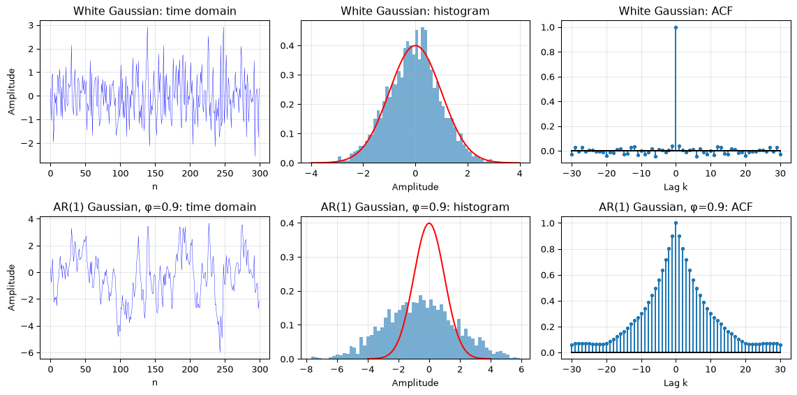
White Gaussian noise has two defining signatures: a bell-shaped amplitude histogram and an autocorrelation that is zero at all nonzero lags. If your ACF shows structure at lag > 0, the noise is not white.
Figure 1: White Gaussian noise: time domain, amplitude distribution, and autocorrelation.
The white case (top row) shows the defining property: \(R_{xx}[0] = 1\) and \(R_{xx}[k] \approx 0\) for \(k \neq 0\). The AR(1) case (bottom) shows the signature of first-order Markov correlation: exponential decay of the ACF with lag, fully characterised by a single number: the lag-1 autocorrelation coefficient.
Colouring: the AR(1) process as simplest correlated noise
Filter white noise through \(x[n] = w[n] + \phi \, x[n-1]\) and you get the AR(1) process: the discrete-time analogue of the Ornstein-Uhlenbeck process (Gardiner 2004). Its ACF decays as \(\phi^{|k|}\) and its PSD is
This single-parameter model is the most-used coloured noise in DSP. For \(|\phi| \lesssim 1\) it produces slow drifts (near-brown); for \(\phi \approx 0\) it is nearly white. The noise whitening topic shows how the Kasdin AR coefficients generalise this to power-law spectra.
Poisson process: shot noise
A Poisson process models independent discrete events occurring at a constant average rate \(\lambda\). Each sample is a count: how many photons hit the detector in this interval, how many electrons cross the barrier. The defining property is that the variance equals the mean:
\[\text{Var}[X] = E[X] = \lambda.\]
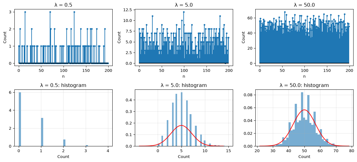
This is fundamentally different from additive Gaussian noise: the noise amplitude is signal-dependent. In low-light imaging, a darker pixel has lower Poisson noise in absolute terms but higher noise relative to signal (\(\sqrt{\lambda}/\lambda = 1/\sqrt{\lambda}\)).
The Schottky formula gives the RMS shot noise current:
\[i_n = \sqrt{2 I q \Delta f} \quad [\text{A}_\text{RMS}]\]
where \(I\) is the DC current in amperes, \(q \approx 1.60 \times 10^{-19}\) C is the electron charge, and \(\Delta f\) is bandwidth. For a photodiode with \(I = 1\ \mu\text{A}\) and \(\Delta f = 1\ \text{kHz}\), this gives \(i_n \approx 18\ \text{pA}_\text{RMS}\).
Figure 2: Poisson (shot) noise at three rates. At high rate it approximates Gaussian; at low rate the discrete, asymmetric nature is visible.
At \(\lambda = 50\) the Poisson is already well-approximated by a Gaussian with \(\sigma = \sqrt{\lambda}\). The Gaussian approximation breaks down at low rates where the discrete, asymmetric nature of the distribution matters.
Lévy / impulse noise: when the tails are heavy
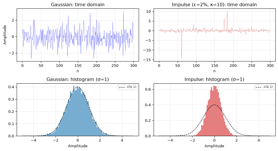
Not all noise is Gaussian. Atmospheric discharge, power-line switching, and ignition systems produce impulse noise: long quiet intervals punctuated by brief, high-amplitude spikes. The amplitude distribution has heavy tails: extreme values are far more probable than a Gaussian would predict.
The contaminated Gaussian mixture is a tractable model:
where \(\epsilon \ll 1\) is the fraction of outlier samples and \(\kappa \gg 1\) is the outlier scale factor. Under this model, a \(3\sigma\) threshold designed for Gaussian noise fires on roughly \((1-\epsilon)\cdot 0.27\% + \epsilon \cdot 76\%\) of samples. For \(\epsilon = 0.02\) and \(\kappa = 10\) that is about 1.8%, roughly 7× more false triggers than the 0.27% a pure Gaussian would produce.
Show the code
n_long =10000x_gauss = gaussian_white(n_long, sigma=1.0, seed=1)x_impulse = levy_impulse_noise(n_long, scale=10.0, outlier_fraction=0.02, seed=1)# Scale to same RMS for fair comparisonx_impulse = x_impulse / np.std(x_impulse)fig, axes = plt.subplots(2, 2, figsize=(10, 5.5))# Time domainaxes[0, 0].plot(x_gauss[:300], 'b-', linewidth=0.3)axes[0, 0].set_title('Gaussian: time domain')axes[0, 0].set_xlabel('n'); axes[0, 0].set_ylabel('Amplitude'); axes[0, 0].grid(True, alpha=0.3)axes[0, 1].plot(x_impulse[:300], 'C3-', linewidth=0.3)axes[0, 1].set_title('Impulse (ε=2%, κ=10): time domain')axes[0, 1].set_xlabel('n'); axes[0, 1].grid(True, alpha=0.3)# Histograms with same x-rangex_lim =5for ax, x, name, color inzip(axes[1], [x_gauss, x_impulse], ['Gaussian', 'Impulse'], ['C0', 'C3']): ax.hist(x, bins=100, range=(-x_lim, x_lim), density=True, alpha=0.6, color=color) xr = np.linspace(-x_lim, x_lim, 200) ax.plot(xr, np.exp(-xr**2/2)/np.sqrt(2*np.pi), 'k--', linewidth=1, label=r'$\mathcal{N}(0,1)$') ax.set_title(f'{name}: histogram (σ=1)') ax.set_xlabel('Amplitude'); ax.legend(fontsize=7); ax.grid(True, alpha=0.3)fig.tight_layout()plt.show()# Verify: Gaussian kurtosis near 0, impulse kurtosis largeinfo_g = characterize(x_gauss)info_i = characterize(x_impulse)print(f"Gaussian excess kurtosis: {info_g['excess_kurtosis']:.2f}")print(f"Impulse excess kurtosis: {info_i['excess_kurtosis']:.1f}")print(f"Max |x| Gaussian: {np.max(np.abs(x_gauss)):.1f}")print(f"Max |x| Impulse: {np.max(np.abs(x_impulse)):.1f}")assert info_i['excess_kurtosis'] >2.0, "Impulse noise should have heavy tails"assert np.max(np.abs(x_impulse)) >3* np.max(np.abs(x_gauss)), "Impulse should have larger excursions"
Figure 3: Impulse noise vs white Gaussian at the same RMS level. The impulse process has the same variance but produces occasional extreme excursions.
Gaussian excess kurtosis:   0.06
Impulse excess kurtosis:    59.0
Max |x| Gaussian:           3.9
Max |x| Impulse:            18.1
The impulse case has the same variance (power) as the Gaussian, but with \(\epsilon = 2\%\) of samples drawn from \(\mathcal{N}(0, 10^2)\). The excess kurtosis quantifies the difference: near zero for Gaussian, large and positive for heavy-tailed noise. This is why robust methods like the median absolute deviation exist: the Gaussian assumption breaks in the presence of impulse noise, and the breakage is not subtle.
Cyclostationary process: when the statistics have a clock
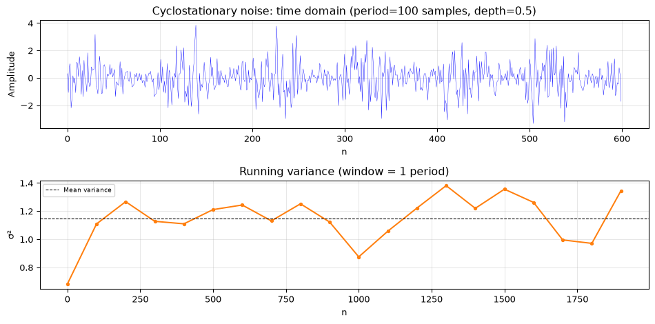
A cyclostationary process is one whose statistical properties (mean, variance, autocorrelation) are periodic. It is not the signal that is periodic; it is the noise statistics.
Every digital system produces cyclostationary noise. A switched-capacitor circuit’s \(kT/C\) noise is modulated by the switch clock. An ADC’s supply rail has noise that follows the conversion cycle. A microcontroller’s GPIO bank draws current on the instruction clock; the resulting ground bounce has a period equal to the clock cycle.
A simple model: white Gaussian noise multiplied by a periodic envelope:
where \(w[n] \sim \mathcal{N}(0, \sigma^2)\) and \(P\) is the clock period in samples. The variance oscillates between \((1-\alpha)^2\sigma^2\) and \((1+\alpha)^2\sigma^2\) with period \(P\).
Show the code
n_long =2000period =100x_cyclo = cyclostationary_noise(n_long, period=period, modulation_depth=0.5, seed=42)fig, axes = plt.subplots(2, 1, figsize=(10, 5))axes[0].plot(x_cyclo[:600], 'b-', linewidth=0.3)axes[0].set_title('Cyclostationary noise: time domain (period=100 samples, depth=0.5)')axes[0].set_xlabel('n'); axes[0].set_ylabel('Amplitude'); axes[0].grid(True, alpha=0.3)# Running variance over windows of exactly one periodn_windows =len(x_cyclo) // periodvar_per_window = np.array([np.var(x_cyclo[i*period:(i+1)*period]) for i inrange(n_windows)])axes[1].plot(np.arange(n_windows) * period, var_per_window, 'C1o-', markersize=3)axes[1].axhline(np.mean(var_per_window), color='k', linestyle='--', linewidth=0.8, label='Mean variance')axes[1].set_title('Running variance (window = 1 period)')axes[1].set_xlabel('n'); axes[1].set_ylabel('σ²'); axes[1].legend(fontsize=7); axes[1].grid(True, alpha=0.3)fig.tight_layout()plt.show()# Verify: variance ratio max/minassert np.max(var_per_window) / np.min(var_per_window) >1.5, "Variance should oscillate measurably"print(f"Variance ratio (max/min): {np.max(var_per_window)/np.min(var_per_window):.2f}")
Figure 4: Cyclostationary noise: white noise with a periodic variance envelope. Bottom: running variance over one-period windows reveals the modulation.
Variance ratio (max/min): 2.03
The practical consequence: averaging measurements taken at different phases of the clock cycle averages different distributions, not different realisations of the same distribution. The \(\sqrt{K}\) improvement law from the basics chapter assumes independent, identically distributed noise: an assumption cyclostationary noise violates.
Telegraph process: burst and RTS noise
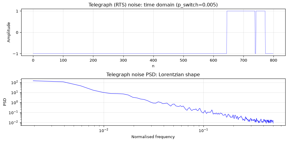
A random telegraph signal (RTS) switches between two discrete levels with a constant per-sample probability \(p\). It is the signature of a single charge trap in a MOSFET gate oxide: the trap fills (current drops), the trap empties (current returns). The result is a two-level signal visible directly in a time series.
The ACF of a telegraph signal with per-sample switching probability \(p\) decays geometrically:
\[R_{xx}[k] = (1 - 2p)^{|k|}\]
(each of the \(|k|\) intervening samples independently flips the sign with probability \(p\), so the expected product is \(((1-p) - p)^{|k|}\)). For small \(p\) this is well approximated by the continuous-time form \(e^{-2pk}\), since \(\ln(1-2p) \approx -2p\),
giving a Lorentzian PSD:
\[S(f) \propto \frac{1}{1 + (f/f_c)^2}\]
with corner frequency \(f_c = p / \pi T_s\). This is not \(1/f\) noise; it has a flat low-frequency plateau and a \(1/f^2\) roll-off above the corner, the spectrum of a single trap.
RTS noise matters because it is not rare in modern semiconductors. A single trap in a small-area transistor (common in image sensor pixels and flash memory cells) can dominate the noise floor. It cannot be averaged away (it is not zero-mean over practical measurement times) and it cannot be filtered with a simple low-pass (its Lorentzian spectrum overlaps the signal band).
Telling them apart from data
Given an unknown noise sequence x, the characterize() function in random_processes.py estimates the key signatures in one call:
The decision tree for identifying an unknown noise source:
Is the ACF flat at nonzero lags? Yes → white (thermal or shot). No → coloured (AR, cyclostationary, or RTS).
Is the distribution symmetric with zero excess kurtosis? Yes → likely Gaussian. No, heavy-tailed → impulse/Lévy.
Does the variance oscillate with a known period? Yes → cyclostationary.
Discrete levels visible in the time series? Yes → telegraph/RTS.
Variance ≈ mean? Yes → Poisson/shot at low rates.
No single number answers “what process is this?”; you need the pattern across distribution, ACF, and PSD together.
On hardware
Characterising noise on a microcontroller is a practical skill: you need to know whether the noise floor in your ADC readings is thermal (unavoidable, Gaussian, flat), quantization (uniform, flat, known from bit depth), or interference (deterministic, not noise at all). See the embedded companion for collecting and analysing noise data on the ESP32-S3 and STM32F4.
Going further
Noise whitening: the AR process is the engine behind \(1/f^\alpha\) noise: the Kasdin coefficients generalise the AR(1) to power-law spectra.
Model-based filtering: the Wiener and Kalman filters are optimal under a Gaussian process assumption; knowing when that assumption holds (and when it does not) is the difference between optimal and dangerous.
Outlier detection: impulse noise is why robust methods exist: the three-sigma rule works for Gaussians and fails for Lévy processes.
ADC noise: the companion topic that takes these process models into the conversion pipeline.
Open question: multiphysics noise decomposition
A real sensor stream contains thermal noise, shot noise, clock noise, and interference simultaneously. Decomposing them blindly (without a known clock, without a noise-only segment, without a model of the sensor physics) is an unsolved problem in the general case. The best practical approach is to eliminate sources one at a time (shield, decouple, filter) and characterise what remains, rather than attempting a blind source separation of noise processes.
References
Gardiner, Crispin W. 2004. Handbook of Stochastic Methods for Physics, Chemistry and the Natural Sciences. 3rd ed. Springer.
Papoulis, Athanasios, and S. Unnikrishna Pillai. 2002. Probability, Random Variables, and Stochastic Processes. 4th ed. McGraw-Hill.
Source Code
---title: "Random Processes"subtitle: "Where noise comes from, stochastically"description-meta: "Where noise comes from, stochastically: the Gaussian, Poisson, heavy-tailed, cyclostationary and telegraph process classes, and telling them apart from data."bibliography: ../../references.bib---Every noise type you meet in DSP is the output of a *random process*: a probabilistic machine that generates sequences of numbers according to some rule. The rule determines everything: the amplitude distribution (Gaussian, Poisson, discrete), the autocorrelation structure (white, coloured, long-range), and what happens if you assume the wrong one.[Noise and SNR](../../basics/03-noise-snr.qmd) introduced the vocabulary: distributions, autocorrelation, white vs coloured noise. This page goes one level deeper: for each major process class, it asks *what physical mechanism produces it, what its statistical signature looks like, and what breaks if you model everything as Gaussian.*The companion module `random_processes.py` provides generators for every process discussed, plus `characterize()` for estimating the signature of an unknown noise sequence.::: {.callout-note title="Prerequisites"}Part of the [noise & stochastic processing arc](../noise-and-stochastic-processing.qmd); the overview gives the reading order.[Noise and SNR](../../basics/03-noise-snr.qmd) (distributions, autocorrelation, power spectral density) and [the frequency domain](../../basics/05-frequency-domain.qmd) (DFT, spectrum).:::::: {.callout-tip title="Code"}The implementation is [`random_processes.py`](random_processes.py). Save [`test_random_processes.py`](test_random_processes.py) beside it and `pytest test_random_processes.py` runs the checks on it.:::```{python}#| echo: falseimport numpy as npimport matplotlib.pyplot as pltfrom random_processes import (gaussian_white, gaussian_ar1, poisson_process, ar_process, levy_impulse_noise, cyclostationary_noise, telegraph_noise, characterize)```<hr>## Why the process class mattersA detection threshold set at $3\sigma$ catches 99.7% of Gaussian samples. Under impulse noise it fires constantly; under a telegraph signal it might never fire at all. A matched filter optimal in white Gaussian noise loses its optimality when the noise is coloured. An averaging strategy that works beautifully for independent Poisson shot noise does nothing for cyclostationary clock noise because the noise *statistics* repeat with the clock, not the measurement.You do not need to classify every noise source you meet, but you do need to know the major types and what they look like in data.<hr>## Gaussian process: the universal defaultA **Gaussian process** is any process whose joint distribution at any set of time points is multivariate normal. The most important special case in DSP is **white Gaussian noise**: each sample is independent, identically distributed $\mathcal{N}(0, \sigma^2)$.### Why it is everywhereThe **central limit theorem** [@papoulis2002probability]: the sum of many independent random effects tends toward a Gaussian, regardless of the individual distributions. Thermal noise in a resistor arises from billions of independent charge-carrier collisions; the aggregate voltage at the terminals is Gaussian to an extraordinarily good approximation.The Johnson-Nyquist formula gives the RMS thermal noise voltage:$$v_n = \sqrt{4 k_B T R \Delta f} \quad [\text{V}_\text{RMS}]$$where $k_B \approx 1.38 \times 10^{-23}$ J/K is Boltzmann's constant, $T$ is absolute temperature in kelvin, $R$ is resistance in ohms, and $\Delta f$ is the measurement bandwidth in Hz. At room temperature (293 K) with $R = 10\ \text{k}\Omega$ and $\Delta f = 20\ \text{kHz}$ (audio band), this gives $v_n \approx 1.8\ \mu\text{V}_\text{RMS}$: the physical noise floor you cannot design away.### What the data looks likeWhite Gaussian noise has two defining signatures: a bell-shaped amplitude histogram and an autocorrelation that is zero at all nonzero lags. If your ACF shows structure at lag > 0, the noise is not white.```{python}#| label: fig-gaussian-process#| fig-cap: "White Gaussian noise: time domain, amplitude distribution, and autocorrelation."rng = np.random.default_rng(42)n =2000x_w = gaussian_white(n, sigma=1.0, seed=42)x_ar = gaussian_ar1(n, phi=0.9, seed=42)fig, axes = plt.subplots(2, 3, figsize=(12, 6))for row, (x, name) inenumerate(zip([x_w, x_ar], ['White Gaussian', 'AR(1) Gaussian, φ=0.9'])): axes[row, 0].plot(x[:300], 'b-', linewidth=0.3) axes[row, 0].set_title(f'{name}: time domain') axes[row, 0].set_xlabel('n'); axes[row, 0].set_ylabel('Amplitude') axes[row, 0].grid(True, alpha=0.3) axes[row, 1].hist(x, bins=60, density=True, alpha=0.6, color='C0') xr = np.linspace(-4, 4, 200) axes[row, 1].plot(xr, np.exp(-xr**2/2)/np.sqrt(2*np.pi), 'r-', linewidth=1.5) axes[row, 1].set_title(f'{name}: histogram') axes[row, 1].set_xlabel('Amplitude'); axes[row, 1].grid(True, alpha=0.3)# ACF lags = np.arange(-30, 31) xc = x - np.mean(x) r = np.correlate(xc, xc, mode='full') r = r / r[len(xc)-1] mid =len(xc) -1 axes[row, 2].stem(lags, r[mid-30:mid+31], linefmt='C0-', markerfmt='C0.', basefmt='k-') axes[row, 2].set_title(f'{name}: ACF') axes[row, 2].set_xlabel('Lag k'); axes[row, 2].grid(True, alpha=0.3)fig.tight_layout()plt.show()```The white case (top row) shows the defining property: $R_{xx}[0] = 1$ and $R_{xx}[k] \approx 0$ for $k \neq 0$. The AR(1) case (bottom) shows the signature of first-order Markov correlation: exponential decay of the ACF with lag, fully characterised by a single number: the lag-1 autocorrelation coefficient.### Colouring: the AR(1) process as simplest correlated noiseFilter white noise through $x[n] = w[n] + \phi \, x[n-1]$ and you get the AR(1) process: the discrete-time analogue of the Ornstein-Uhlenbeck process [@gardiner2004handbook]. Its ACF decays as $\phi^{|k|}$ and its PSD is$$S(f) = \frac{\sigma_w^2}{|1 - \phi e^{-j2\pi f}|^2}.$$This single-parameter model is the most-used coloured noise in DSP. For $|\phi| \lesssim 1$ it produces slow drifts (near-brown); for $\phi \approx 0$ it is nearly white. The [noise whitening topic](../noise-whitening/index.qmd) shows how the Kasdin AR coefficients generalise this to power-law spectra.<hr>## Poisson process: shot noiseA **Poisson process** models independent discrete events occurring at a constant average rate $\lambda$. Each sample is a count: how many photons hit the detector in this interval, how many electrons cross the barrier. The defining property is that the variance equals the mean:$$\text{Var}[X] = E[X] = \lambda.$$This is fundamentally different from additive Gaussian noise: the noise amplitude is *signal-dependent*. In low-light imaging, a darker pixel has lower Poisson noise in absolute terms but higher noise *relative to signal* ($\sqrt{\lambda}/\lambda = 1/\sqrt{\lambda}$).The Schottky formula gives the RMS shot noise current:$$i_n = \sqrt{2 I q \Delta f} \quad [\text{A}_\text{RMS}]$$where $I$ is the DC current in amperes, $q \approx 1.60 \times 10^{-19}$ C is the electron charge, and $\Delta f$ is bandwidth. For a photodiode with $I = 1\ \mu\text{A}$ and $\Delta f = 1\ \text{kHz}$, this gives $i_n \approx 18\ \text{pA}_\text{RMS}$.```{python}#| label: fig-poisson-process#| fig-cap: "Poisson (shot) noise at three rates. At high rate it approximates Gaussian; at low rate the discrete, asymmetric nature is visible."n_plot =200rates = [0.5, 5.0, 50.0]fig, axes = plt.subplots(2, 3, figsize=(12, 5.5))for j, rate inenumerate(rates): x = poisson_process(n_plot, rate=rate, seed=42) axes[0, j].stem(np.arange(n_plot), x, linefmt='C0-', markerfmt='C0.', basefmt='k-') axes[0, j].set_title(f'λ = {rate}') axes[0, j].set_xlabel('n'); axes[0, j].set_ylabel('Count') x_long = poisson_process(20000, rate=rate, seed=42) axes[1, j].hist(x_long, bins=40, density=True, alpha=0.6, color='C0')# Overlay Gaussian approximation for higher ratesif rate >2: xr = np.linspace(rate -4*np.sqrt(rate), rate +4*np.sqrt(rate), 150) axes[1, j].plot(xr, np.exp(-(xr-rate)**2/(2*rate))/np.sqrt(2*np.pi*rate), 'r-', linewidth=1.5) axes[1, j].set_title(f'λ = {rate}: histogram') axes[1, j].set_xlabel('Count'); axes[1, j].grid(True, alpha=0.3)fig.tight_layout()plt.show()```At $\lambda = 50$ the Poisson is already well-approximated by a Gaussian with $\sigma = \sqrt{\lambda}$. The Gaussian approximation breaks down at low rates where the discrete, asymmetric nature of the distribution matters.<hr>## Lévy / impulse noise: when the tails are heavyNot all noise is Gaussian. Atmospheric discharge, power-line switching, and ignition systems produce **impulse noise**: long quiet intervals punctuated by brief, high-amplitude spikes. The amplitude distribution has *heavy tails*: extreme values are far more probable than a Gaussian would predict.The contaminated Gaussian mixture is a tractable model:$$p(x) = (1-\epsilon)\,\mathcal{N}(0,\sigma^2) + \epsilon\,\mathcal{N}(0,\kappa^2\sigma^2)$$where $\epsilon \ll 1$ is the fraction of outlier samples and $\kappa \gg 1$ is the outlier scale factor. Under this model, a $3\sigma$ threshold designed for Gaussian noise fires on roughly $(1-\epsilon)\cdot 0.27\% + \epsilon \cdot 76\%$ of samples. For $\epsilon = 0.02$ and $\kappa = 10$ that is about 1.8%, roughly 7× more false triggers than the 0.27% a pure Gaussian would produce.```{python}#| label: fig-impulse-noise#| fig-cap: "Impulse noise vs white Gaussian at the same RMS level. The impulse process has the same variance but produces occasional extreme excursions."n_long =10000x_gauss = gaussian_white(n_long, sigma=1.0, seed=1)x_impulse = levy_impulse_noise(n_long, scale=10.0, outlier_fraction=0.02, seed=1)# Scale to same RMS for fair comparisonx_impulse = x_impulse / np.std(x_impulse)fig, axes = plt.subplots(2, 2, figsize=(10, 5.5))# Time domainaxes[0, 0].plot(x_gauss[:300], 'b-', linewidth=0.3)axes[0, 0].set_title('Gaussian: time domain')axes[0, 0].set_xlabel('n'); axes[0, 0].set_ylabel('Amplitude'); axes[0, 0].grid(True, alpha=0.3)axes[0, 1].plot(x_impulse[:300], 'C3-', linewidth=0.3)axes[0, 1].set_title('Impulse (ε=2%, κ=10): time domain')axes[0, 1].set_xlabel('n'); axes[0, 1].grid(True, alpha=0.3)# Histograms with same x-rangex_lim =5for ax, x, name, color inzip(axes[1], [x_gauss, x_impulse], ['Gaussian', 'Impulse'], ['C0', 'C3']): ax.hist(x, bins=100, range=(-x_lim, x_lim), density=True, alpha=0.6, color=color) xr = np.linspace(-x_lim, x_lim, 200) ax.plot(xr, np.exp(-xr**2/2)/np.sqrt(2*np.pi), 'k--', linewidth=1, label=r'$\mathcal{N}(0,1)$') ax.set_title(f'{name}: histogram (σ=1)') ax.set_xlabel('Amplitude'); ax.legend(fontsize=7); ax.grid(True, alpha=0.3)fig.tight_layout()plt.show()# Verify: Gaussian kurtosis near 0, impulse kurtosis largeinfo_g = characterize(x_gauss)info_i = characterize(x_impulse)print(f"Gaussian excess kurtosis: {info_g['excess_kurtosis']:.2f}")print(f"Impulse excess kurtosis: {info_i['excess_kurtosis']:.1f}")print(f"Max |x| Gaussian: {np.max(np.abs(x_gauss)):.1f}")print(f"Max |x| Impulse: {np.max(np.abs(x_impulse)):.1f}")assert info_i['excess_kurtosis'] >2.0, "Impulse noise should have heavy tails"assert np.max(np.abs(x_impulse)) >3* np.max(np.abs(x_gauss)), "Impulse should have larger excursions"```The impulse case has the same variance (power) as the Gaussian, but with $\epsilon = 2\%$ of samples drawn from $\mathcal{N}(0, 10^2)$. The excess kurtosis quantifies the difference: near zero for Gaussian, large and positive for heavy-tailed noise. This is why robust methods like the [median absolute deviation](../outlier-detection/index.qmd) exist: the Gaussian assumption breaks in the presence of impulse noise, and the breakage is not subtle.<hr>## Cyclostationary process: when the statistics have a clockA **cyclostationary** process is one whose statistical properties (mean, variance, autocorrelation) are periodic. It is not the *signal* that is periodic; it is the *noise statistics*.Every digital system produces cyclostationary noise. A switched-capacitor circuit's $kT/C$ noise is modulated by the switch clock. An ADC's supply rail has noise that follows the conversion cycle. A microcontroller's GPIO bank draws current on the instruction clock; the resulting ground bounce has a period equal to the clock cycle.A simple model: white Gaussian noise multiplied by a periodic envelope:$$x[n] = w[n] \cdot \bigl(1 + \alpha \sin(2\pi n / P)\bigr)$$where $w[n] \sim \mathcal{N}(0, \sigma^2)$ and $P$ is the clock period in samples. The variance oscillates between $(1-\alpha)^2\sigma^2$ and $(1+\alpha)^2\sigma^2$ with period $P$.```{python}#| label: fig-cyclostationary#| fig-cap: "Cyclostationary noise: white noise with a periodic variance envelope. Bottom: running variance over one-period windows reveals the modulation."n_long =2000period =100x_cyclo = cyclostationary_noise(n_long, period=period, modulation_depth=0.5, seed=42)fig, axes = plt.subplots(2, 1, figsize=(10, 5))axes[0].plot(x_cyclo[:600], 'b-', linewidth=0.3)axes[0].set_title('Cyclostationary noise: time domain (period=100 samples, depth=0.5)')axes[0].set_xlabel('n'); axes[0].set_ylabel('Amplitude'); axes[0].grid(True, alpha=0.3)# Running variance over windows of exactly one periodn_windows =len(x_cyclo) // periodvar_per_window = np.array([np.var(x_cyclo[i*period:(i+1)*period]) for i inrange(n_windows)])axes[1].plot(np.arange(n_windows) * period, var_per_window, 'C1o-', markersize=3)axes[1].axhline(np.mean(var_per_window), color='k', linestyle='--', linewidth=0.8, label='Mean variance')axes[1].set_title('Running variance (window = 1 period)')axes[1].set_xlabel('n'); axes[1].set_ylabel('σ²'); axes[1].legend(fontsize=7); axes[1].grid(True, alpha=0.3)fig.tight_layout()plt.show()# Verify: variance ratio max/minassert np.max(var_per_window) / np.min(var_per_window) >1.5, "Variance should oscillate measurably"print(f"Variance ratio (max/min): {np.max(var_per_window)/np.min(var_per_window):.2f}")```The practical consequence: averaging measurements taken at different phases of the clock cycle averages *different distributions*, not different realisations of the same distribution. The $\sqrt{K}$ improvement law from the basics chapter assumes independent, identically distributed noise: an assumption cyclostationary noise violates.<hr>## Telegraph process: burst and RTS noiseA **random telegraph signal** (RTS) switches between two discrete levels with a constant per-sample probability $p$. It is the signature of a single charge trap in a MOSFET gate oxide: the trap fills (current drops), the trap empties (current returns). The result is a two-level signal visible directly in a time series.The ACF of a telegraph signal with per-sample switching probability $p$ decays geometrically:$$R_{xx}[k] = (1 - 2p)^{|k|}$$(each of the $|k|$ intervening samples independently flips the sign with probability $p$, so the expected product is $((1-p) - p)^{|k|}$). For small $p$ this is well approximated by the continuous-time form $e^{-2pk}$, since $\ln(1-2p) \approx -2p$,giving a Lorentzian PSD:$$S(f) \propto \frac{1}{1 + (f/f_c)^2}$$with corner frequency $f_c = p / \pi T_s$. This is not $1/f$ noise; it has a flat low-frequency plateau and a $1/f^2$ roll-off above the corner, the spectrum of a single trap.```{python}#| label: fig-telegraph#| fig-cap: "Random telegraph signal (RTS). Two discrete levels with random switching: the signature of a single charge trap in a semiconductor."n_long =5000x_rts = telegraph_noise(n_long, p_switch=0.005, levels=(-1.0, 1.0), seed=42)fig, axes = plt.subplots(2, 1, figsize=(10, 5))axes[0].plot(x_rts[:800], 'b-', linewidth=0.4)axes[0].set_title('Telegraph (RTS) noise: time domain (p_switch=0.005)')axes[0].set_xlabel('n'); axes[0].set_ylabel('Amplitude')axes[0].set_yticks([-1, 0, 1]); axes[0].grid(True, alpha=0.3)# PSDfrom scipy.signal import welchf, psd = welch(x_rts, 1.0, nperseg=512)axes[1].loglog(f[1:], psd[1:], 'b-', linewidth=0.8)axes[1].set_title('Telegraph noise PSD: Lorentzian shape')axes[1].set_xlabel('Normalised frequency'); axes[1].set_ylabel('PSD')axes[1].grid(True, alpha=0.3)fig.tight_layout()plt.show()# Verify only two levelsinfo = characterize(x_rts)print(f"Unique values: {np.unique(x_rts)}")print(f"ACF lag-1: {info['acf_lag1']:.3f}")print(f"ACF lag-5: {info['acf_lag5']:.3f}")assert info['acf_lag1'] >0.5, "Slow switching should give strong lag-1 correlation"```RTS noise matters because it is *not rare* in modern semiconductors. A single trap in a small-area transistor (common in image sensor pixels and flash memory cells) can dominate the noise floor. It cannot be averaged away (it is not zero-mean over practical measurement times) and it cannot be filtered with a simple low-pass (its Lorentzian spectrum overlaps the signal band).<hr>## Telling them apart from dataGiven an unknown noise sequence `x`, the `characterize()` function in [`random_processes.py`](random_processes.py) estimates the key signatures in one call:```{python}#| label: fig-characterize-demo#| fig-cap: "Characterising an unknown noise sequence: distribution moments, ACF shape, and PSD slope together identify the process class."for name, x_gen in [('White Gaussian', gaussian_white(10000, seed=1)), ('AR(1) φ=0.9', gaussian_ar1(10000, phi=0.9, seed=1)), ('Impulse ε=2%', levy_impulse_noise(10000, scale=10, outlier_fraction=0.02, seed=1))]: info = characterize(x_gen)print(f"\n{name}:")print(f" mean={info['mean']:.3f}, std={info['std']:.3f}")print(f" skewness={info['skewness']:.2f}, excess kurtosis={info['excess_kurtosis']:.2f}")print(f" ACF lag-1={info['acf_lag1']:.3f}, lag-2={info['acf_lag2']:.3f}")print(f" PSD slope={info['psd_slope']:.2f} (R²={info['psd_r2']:.2f})")print(f" zero-mean={info['is_zero_mean']}, symmetric={info['is_symmetric']}")```The decision tree for identifying an unknown noise source:1. **Is the ACF flat at nonzero lags?** Yes → white (thermal or shot). No → coloured (AR, cyclostationary, or RTS).2. **Is the distribution symmetric with zero excess kurtosis?** Yes → likely Gaussian. No, heavy-tailed → impulse/Lévy.3. **Does the variance oscillate with a known period?** Yes → cyclostationary.4. **Discrete levels visible in the time series?** Yes → telegraph/RTS.5. **Variance ≈ mean?** Yes → Poisson/shot at low rates.No single number answers "what process is this?"; you need the pattern across distribution, ACF, and PSD together.<hr>## On hardwareCharacterising noise on a microcontroller is a practical skill: you need to know whether the noise floor in your ADC readings is thermal (unavoidable, Gaussian, flat), quantization (uniform, flat, known from bit depth), or interference (deterministic, not noise at all). See the [embedded companion](embedded.qmd) for collecting and analysing noise data on the ESP32-S3 and STM32F4.<hr>## Going further- **[Noise whitening](../noise-whitening/index.qmd)**: the AR process is the engine behind $1/f^\alpha$ noise: the Kasdin coefficients generalise the AR(1) to power-law spectra.- **[Model-based filtering](../model-based-filtering/index.qmd)**: the Wiener and Kalman filters are optimal *under a Gaussian process assumption*; knowing when that assumption holds (and when it does not) is the difference between optimal and dangerous.- **[Outlier detection](../outlier-detection/index.qmd)**: impulse noise is why robust methods exist: the three-sigma rule works for Gaussians and fails for Lévy processes.- **[ADC noise](../adc-noise/index.qmd)**: the companion topic that takes these process models into the conversion pipeline.::: {.callout-warning title="Open question: multiphysics noise decomposition"}A real sensor stream contains thermal noise, shot noise, clock noise, and interference simultaneously. Decomposing them blindly (without a known clock, without a noise-only segment, without a model of the sensor physics) is an unsolved problem in the general case. The best practical approach is to eliminate sources one at a time (shield, decouple, filter) and characterise what remains, rather than attempting a blind source separation of noise processes.:::## References::: {#refs}:::