When you know the statistics of the signal and the noise, optimal estimation follows: Wiener and Kalman
A classical filter is designed in the frequency domain: you decide which bands to keep and which to reject, and you do not much care what the signal is, only where it lives in frequency. Model-based filtering asks a different question. Suppose you have a statistical model of the signal you want and of the noise corrupting it. What is the best possible estimate of the signal, in the mean-square sense, that a linear filter can produce?
That question has a clean answer, and two famous filters realise it. The Wiener filter answers it for a stationary signal in stationary noise: it is the linear minimum-mean-square-error (MMSE) estimator, and it falls out of a set of linear equations built from the signals’ correlations. The Kalman filter answers it for a signal that evolves according to a dynamical model, recursively, updating its estimate every time a new measurement arrives. Both replace “which frequencies do I trust” with “given everything I know about how this signal and this noise behave, what is my best guess.”
Prerequisites and family
This topic builds on correlation and the statistics of random signals and the frequency domain. It is the third member of an optimal-filtering family: the matched filter detects a known waveform in noise (maximising output SNR), noise whitening flattens a coloured spectrum, and the filters here estimate a random signal whose statistics you model. The Wiener filter is also the batch ancestor of the adaptive filters, which learn the same optimum online when the statistics are unknown.
Take the simplest estimation problem. A desired signal \(d[n]\) is observed in additive noise \(v[n]\),
\[x[n] = d[n] + v[n],\]
with \(d\) and \(v\) both wide-sense stationary and uncorrelated with each other. We want to recover \(d[n]\) from the observations using a length-\(M\) FIR filter,
\[\hat{d}[n] = \sum_{k=0}^{M-1} w[k]\, x[n-k],\]
and we want the coefficients \(w[k]\) that make the estimate as close to \(d[n]\) as possible, measuring “close” by the mean-square error \(J = \mathbb{E}\big[(d[n] - \hat{d}[n])^2\big]\).
The orthogonality principle
The error surface \(J(w)\) is a quadratic bowl, so it has a single minimum where the gradient vanishes. Setting \(\partial J / \partial w[j] = 0\) gives a condition with a clean interpretation: at the optimum, the estimation error is orthogonal to every input sample the filter used,
The filter has extracted everything about \(d[n]\) that is linearly predictable from \(\{x[n], \dots, x[n-M+1]\}\); whatever error remains is uncorrelated with the data, so no linear adjustment of the taps could reduce it further.
The Wiener-Hopf equations
Expanding the orthogonality condition turns it into a linear system. Writing \(r_{xx}[\ell] = \mathbb{E}[x[n]x[n-\ell]]\) for the autocorrelation of the observations and \(r_{dx}[\ell] = \mathbb{E}[d[n]x[n-\ell]]\) for the cross-correlation between desired and observed signals,
In matrix form these are the Wiener-Hopf normal equations,
\[\mathbf{R}_x\, \mathbf{w} = \mathbf{r}_{dx},\]
where \(\mathbf{R}_x\) is the \(M \times M\) symmetric Toeplitz autocorrelation matrix and \(\mathbf{r}_{dx}\) is the cross-correlation vector. Solving for \(\mathbf{w} = \mathbf{R}_x^{-1}\mathbf{r}_{dx}\) gives the optimal filter, and the error it leaves behind has the closed form
with \(\sigma_d^2 = \mathbb{E}[d[n]^2]\) the power of the desired signal. This \(J_{\min}\) is a hard floor for linear estimation: among filters that form a weighted sum of the inputs, no FIR filter of this length can estimate \(d\) with smaller mean-square error. (When the signal is non-Gaussian a nonlinear function of the same inputs can do better; the Wiener filter is the best linear one.)
It hits the predicted floor
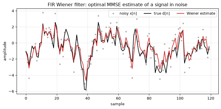
The demo takes a desired signal with memory (a first-order autoregressive process, \(d[n] = 0.8\,d[n-1] + e[n]\), which is lowpass and partly predictable), buries it in white noise at an input SNR of about 4.4 dB, designs the 16-tap Wiener filter from the true correlations, and runs it on a long record. The MSE it actually achieves should match the \(J_{\min}\) the formula predicts.
Show the code
rng = np.random.default_rng(0)a, sigma_e, sigma_v, M =0.8, 1.0, 1.0, 16# True correlations of d (AR1) and x = d + v.var_d = sigma_e**2/ (1- a**2)lags = np.arange(M)rdd = var_d * a**lagsrxx = rdd.copy(); rxx[0] += sigma_v**2# add white-noise power on the diagonal lagrdx = rdd # d uncorrelated with vw = wiener_hopf(rxx, rdx)j_min = wiener_min_mse(rxx, rdx, var_d)# Long realisation to measure the achieved MSE.n =100_000e = rng.standard_normal(n) * sigma_ed = np.zeros(n)for k inrange(1, n): d[k] = a * d[k -1] + e[k]x = d + rng.standard_normal(n) * sigma_vd_hat = wiener_apply(w, x)measured = np.mean((d[M:] - d_hat[M:])**2)in_mse = np.mean((d[M:] - x[M:])**2)assert measured < in_mse # the filter must helpassert np.isclose(measured, j_min, rtol=0.05) # and hit the predicted floorprint(f"input MSE = {in_mse:.3f} Wiener MSE = {measured:.3f} predicted J_min = {j_min:.3f}")print(f"error reduced by {in_mse / measured:.2f}x")seg =slice(200, 320)fig, ax = plt.subplots(figsize=(8, 4))ax.plot(x[seg], color='C7', alpha=0.5, marker='.', linestyle='none', label='noisy x[n]')ax.plot(d[seg], color='k', linewidth=1.5, label='true d[n]')ax.plot(d_hat[seg], color='C3', linewidth=1.5, label='Wiener estimate')ax.set_xlabel('sample'); ax.set_ylabel('amplitude')ax.set_title('FIR Wiener filter: optimal MMSE estimate of a signal in noise')ax.legend(fontsize=9, ncol=3); ax.grid(True, alpha=0.3)fig.tight_layout()plt.show()
input MSE = 1.005   Wiener MSE = 0.578   predicted J_min = 0.578
error reduced by 1.74x
Figure 1: A 16-tap Wiener filter recovering an AR(1) signal from white noise. The noisy observations (grey) scatter widely around the true signal (black); the Wiener estimate (red) tracks it closely. The MSE the filter achieves matches the J_min the normal equations predict, confirming the filter is optimal, not merely good.
The frequency-domain view
If we drop the causal, finite-length constraint and allow a non-causal filter of unlimited extent, the Wiener-Hopf equations become a single division in the frequency domain. The optimal frequency response is
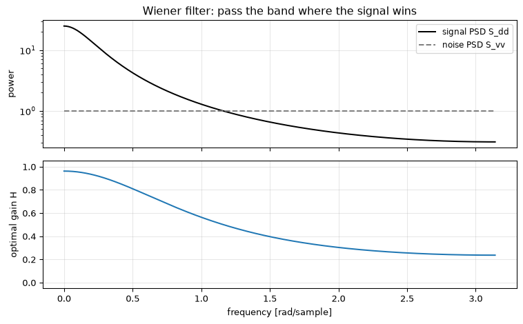
where \(S_{dd}\) and \(S_{vv}\) are the power spectral densities of signal and noise (the second equality uses \(d \perp v\)). This is the Wiener filter in its most readable form: at every frequency it computes the local signal-to-noise ratio and passes that fraction of the input. Where the signal dominates, \(H \approx 1\) and the band passes through; where the noise dominates, \(H \approx 0\) and the band is suppressed. The gain is always between 0 and 1, a soft, frequency-by-frequency SNR gate rather than a hard brick wall.
Show the code
w_grid = np.linspace(0, np.pi, 400)# AR(1) signal PSD: S_dd(w) = sigma_e^2 / |1 - a e^{-jw}|^2S_dd = sigma_e**2/ np.abs(1- a * np.exp(-1j* w_grid))**2S_vv = np.full_like(w_grid, sigma_v**2)H = wiener_freq(S_dd, S_vv)assert np.all((H >=0) & (H <=1))fig, (ax1, ax2) = plt.subplots(2, 1, figsize=(8, 5), sharex=True)ax1.semilogy(w_grid, S_dd, color='k', label='signal PSD S_dd')ax1.semilogy(w_grid, S_vv, color='C7', linestyle='--', label='noise PSD S_vv')ax1.set_ylabel('power'); ax1.legend(fontsize=9); ax1.grid(True, alpha=0.3)ax1.set_title('Wiener filter: pass the band where the signal wins')ax2.plot(w_grid, H, color='C0')ax2.set_xlabel('frequency [rad/sample]'); ax2.set_ylabel('optimal gain H')ax2.set_ylim(-0.05, 1.05); ax2.grid(True, alpha=0.3)fig.tight_layout()plt.show()
Figure 2: The frequency-domain Wiener filter as a soft SNR gate. A lowpass signal spectrum (the AR(1) signal) sits on a flat white-noise floor. The optimal gain H = S_dd / (S_dd + S_vv) is near 1 at low frequencies where the signal is strong and rolls down at high frequencies where the noise dominates. It never overshoots 1 or goes negative.
The Wiener filter has one practical catch: it needs the correlations (or spectra) of the signal and noise, and it assumes they are stationary. When you do not know them, you estimate them from data, which is exactly what the adaptive filters do online. And when the signal is not stationary but instead evolves according to a known dynamical law, the right tool is the Kalman filter.
The Kalman filter
The Wiener filter estimates a stationary signal in one batch. Many real signals are not stationary: a tracked object moves, a temperature drifts, a battery discharges. For these we write down a state-space model of how the signal evolves and let the filter carry its estimate forward in step with the system, folding in each new measurement as it arrives. That recursion is the Kalman filter, and it is the workhorse of navigation, tracking, and sensor fusion.
Nature’s version of predicting before you measure
The move that makes this filter work is predicting the state before looking at the new measurement, and it turns out to be an interception strategy a dragonfly already uses. Tracking head and body orientation through prey-capture flights showed that a dragonfly rotates its head to where the prey is going to be, and steers its body from that prediction, using what the authors identify as internal models of both its own body dynamics and the prey’s motion; vision is reserved mainly for correcting when the prey does something unexpected (Mischiati et al. 2015). Predict from a model, then use the sensor for the residual.
The correspondence is structural, not literal: nothing in the insect propagates a covariance matrix or computes a Kalman gain, and the paper claims internal models, not optimal estimation. What carries over is why prediction pays. A purely reactive tracker is always one sensory delay behind a moving target, and an interception that must be committed before the prey reacts cannot afford that lag. Prediction converts the sensor’s job from measure everything into correct a good guess, which is exactly what the two-step recursion below formalises.
The state-space model
The system carries a hidden state \(\mathbf{x}_k\) (a vector: position and velocity, say) that evolves linearly, and we observe a noisy linear function of it:
Here \(\mathbf{F}\) is the state-transition matrix (the dynamics), \(\mathbf{H}\) maps the state to what we can measure, \(\mathbf{Q}\) is the process-noise covariance (how much the model is buffeted by unmodelled forces), and \(\mathbf{R}\) is the measurement-noise covariance (how noisy the sensor is). The filter tracks not only a state estimate \(\hat{\mathbf{x}}\) but its error covariance \(\mathbf{P}\), a running statement of how uncertain it is.
Predict, then update
Each step has two phases. Predict rolls the estimate forward through the dynamics and lets the uncertainty grow by the process noise:
Update then corrects the prediction with the new measurement. The correction is driven by the innovation\(\tilde{\mathbf{y}}_k\) (how much the measurement disagrees with the prediction), scaled by the Kalman gain\(\mathbf{K}_k\):
The gain is the filter’s confidence dial. When the measurement is clean (\(\mathbf{R}\) small), \(\mathbf{K}\) is large and the filter trusts the data; when the measurement is noisy (\(\mathbf{R}\) large), \(\mathbf{K}\) shrinks and the filter leans on its model. It sets that balance automatically, from the covariances, at every step.
The truck on rails
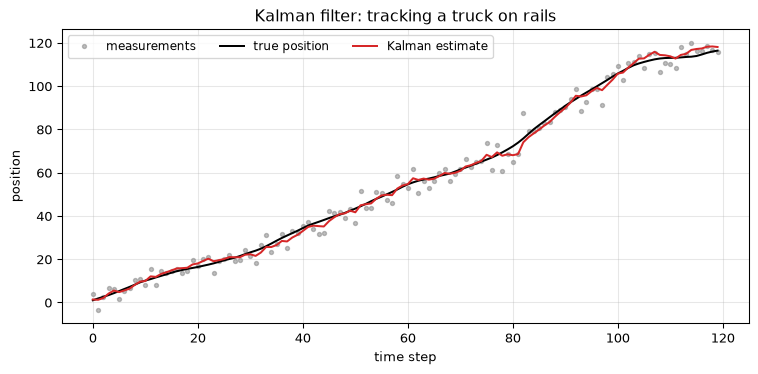
The textbook example is a truck on frictionless, straight rails. Its state is position and velocity, \(\mathbf{x} = [p, \dot p]^{\mathsf T}\). Between time steps an unknown acceleration buffets it, modelled as white noise of standard deviation \(\sigma_a\); we measure only its position, with sensor noise \(\sigma_z\). From the kinematics, the model matrices are
where \(\mathbf{Q} = \mathbf{G}\mathbf{G}^{\mathsf T}\sigma_a^2\) with \(\mathbf{G} = [\Delta t^2/2,\ \Delta t]^{\mathsf T}\) is the standard discrete white-noise-acceleration covariance: a constant acceleration over \(\Delta t\) shifts position by \(\tfrac12 a\,\Delta t^2\) and velocity by \(a\,\Delta t\). The filter is never told the velocity, yet it infers it from the position measurements and uses it to predict ahead.
Figure 3: Kalman filter tracking a truck on rails from noisy position measurements alone. The measurements (grey) are scattered by sensor noise; the filter’s estimate (red) stays close to the true position (black), and its RMSE is well below the measurement RMSE. The filter recovers velocity it never directly observes and uses it to smooth the position.
The filter knows how wrong it is
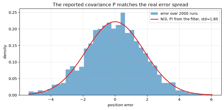
The covariance \(\mathbf{P}_{k\mid k}\) the filter reports is not decoration: it is a genuine prediction of the filter’s own error, and it can be checked. If we run the same truck many times with fresh noise and collect the position error at a fixed late step, that error spread should match the standard deviation \(\sqrt{P_{11}}\) the filter claims. We check it at a late step deliberately: there the filter has reached steady state and the arbitrary initial \(\mathbf{P}_0\) has washed out, so the calibration is exact regardless of how we seeded it. The demo runs 2000 independent trucks and compares.
Show the code
dt, sigma_a, sigma_z =1.0, 0.3, 3.0F, H, Q, R = cv_model(dt, sigma_a, sigma_z)steps =40x0 = np.array([0.0, 1.0]); P0 = np.eye(2)rng = np.random.default_rng(7)runs =2000final_err = np.empty(runs)P_reported =Nonefor r inrange(runs): xs_true, z = simulate_cv(F, H, Q, R, x0, steps, rng) xs, Ps = kalman_filter(z, F, H, Q, R, x0, P0) final_err[r] = xs_true[-1, 0] - xs[-1, 0] P_reported = Ps[-1]std_reported = np.sqrt(P_reported[0, 0])std_empirical = final_err.std()assert np.isclose(std_empirical, std_reported, rtol=0.1)print(f"reported position std sqrt(P) = {std_reported:.3f} empirical error std = {std_empirical:.3f}")fig, ax = plt.subplots(figsize=(8, 4))ax.hist(final_err, bins=40, density=True, color='C0', alpha=0.6, label='error over 2000 runs')grid = np.linspace(final_err.min(), final_err.max(), 200)gauss = np.exp(-grid**2/ (2* std_reported**2)) / (std_reported * np.sqrt(2* np.pi))ax.plot(grid, gauss, color='C3', linewidth=2, label=f'N(0, P) from the filter, std={std_reported:.2f}')ax.set_xlabel('position error'); ax.set_ylabel('density')ax.set_title('The reported covariance P matches the real error spread')ax.legend(fontsize=9); ax.grid(True, alpha=0.3)fig.tight_layout()plt.show()
Figure 4: The Kalman filter’s reported uncertainty is calibrated. Across 2000 independent runs, the histogram of the filter’s position error at the final step is a Gaussian whose width matches the standard deviation sqrt(P) the filter computed from the covariance recursion alone, never having seen the errors. The filter does not just estimate the state; it correctly estimates its own accuracy.
It settles to a constant gain
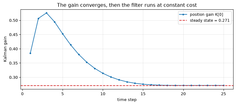
For a time-invariant model (\(\mathbf{F}, \mathbf{H}, \mathbf{Q}, \mathbf{R}\) all constant) the covariance \(\mathbf{P}\) and gain \(\mathbf{K}\) do not change forever. They converge to fixed values, the solution of the discrete algebraic Riccati equation, after which every step uses the same gain. That steady-state gain can be computed once, offline, and baked into the implementation, which turns the per-sample arithmetic into a fixed linear update with no matrix inverse. This is the alpha-beta filter (alpha and beta being the constant position and velocity gains), the form a microcontroller runs, and it is the bridge to the hardware page.
Show the code
dt, sigma_a, sigma_z =1.0, 0.2, 4.0F, H, Q, R = cv_model(dt, sigma_a, sigma_z)K_inf, P_inf = steady_state_gain(F, H, Q, R)# Track the per-step gain by reading P back out of a run.P =5.0* np.eye(2); I = np.eye(2)gains = []for _ inrange(25): P = F @ P @ F.T + Q S = H @ P @ H.T + R K = P @ H.T @ np.linalg.inv(S) P = (I - K @ H) @ P gains.append(K[0, 0])assertabs(gains[-1] - K_inf[0, 0]) <1e-3# converged to the Riccati steady statefig, ax = plt.subplots(figsize=(8, 3.6))ax.plot(range(1, 26), gains, color='C0', marker='o', ms=3, label='position gain K[0]')ax.axhline(K_inf[0, 0], color='C3', linestyle='--', label=f'steady state = {K_inf[0,0]:.3f}')ax.set_xlabel('time step'); ax.set_ylabel('Kalman gain')ax.set_title('The gain converges, then the filter runs at constant cost')ax.legend(fontsize=9); ax.grid(True, alpha=0.3)fig.tight_layout()plt.show()
Figure 5: The Kalman gain is transient, then constant. Starting from an uncertain initial covariance, the position-gain element first overshoots to nearly twice the steady-state value, then settles over a dozen-odd steps to the value computed independently from the Riccati recursion (dashed). After convergence the filter is a fixed-gain linear update, which is what makes it cheap to run on a microcontroller.
Going further
Nonlinear systems break the linear assumption. Both Wiener and Kalman are linear optimal filters. When the dynamics or the measurement are nonlinear (a radar measures range and bearing, not Cartesian position), the extended Kalman filter linearises the model about the current estimate at each step, and the unscented Kalman filter propagates a small set of sample points through the true nonlinearity instead. Both are approximations, and neither is guaranteed optimal; for strongly nonlinear or multimodal problems a particle filter may be needed.
The optimality is only as good as the model. The Kalman filter is provably optimal if the model matches reality, the noise is white and Gaussian, and \(\mathbf{Q}\) and \(\mathbf{R}\) are correct. When they are not, the filter can become overconfident: its reported \(\mathbf{P}\) shrinks while the true error does not, and the gain drops so far that the filter stops listening to measurements and diverges. Tuning \(\mathbf{Q}\) and \(\mathbf{R}\) honestly, and sometimes inflating them deliberately, is the practical heart of getting a Kalman filter to work.
Numerical conditioning matters. The simple covariance update \(\mathbf{P}_{k\mid k} = (\mathbf{I} - \mathbf{K}\mathbf{H})\mathbf{P}_{k\mid k-1}\) used above is correct only for the optimal gain and can lose symmetry or positive-definiteness in finite precision. The Joseph form of the update is algebraically equal but numerically robust, and square-root filters propagate a factor of \(\mathbf{P}\) instead of \(\mathbf{P}\) itself to keep it positive-definite. These are the finite word-length concerns of state estimation.
Recursion connects to adaptation and to Bayes. The Kalman filter is exactly recursive Bayesian estimation for a linear-Gaussian model: each step is a Bayesian prior-to-posterior update. Run with a forgetting factor on a regression state, it becomes the recursive least squares adaptive filter. The threads tie together: matched, Wiener, Kalman, and RLS are all the same MMSE idea seen from different angles. The recursive-estimation page walks that lineage in full (batch least squares to RLS to Kalman-as-recursive-MMSE) and pins the equivalences with tests.
Estimation is only half of a control loop. This page treats the Kalman filter purely as an estimator: given measurements, recover the state. In a servo or a motor drive that estimate then drives an actuator, which is the province of control systems rather than signal processing. The same recursive structure reappears there as the state observer: the deterministic Luenberger observer places the error-dynamics poles by hand, and the Kalman filter is the stochastic-optimal observer for the same structure. An observer is often used exactly as here, to clean a measurement, for instance to reduce encoder-quantization noise on a position signal before closing the loop. Feedforward compensation, which adds a model of the known driving input so the loop does not have to wait for an error to build up, attacks tracking lag from the control side, and field-oriented control of a PMSM is a classic application that leans on both an observer and feedforward. These cross from DSP into control systems and are out of scope for this workshop; for that continuation, Åström and Murray’s Feedback Systems (freely available at fbswiki.org) is a good starting point.
References
The Wiener filter and the orthogonality principle follow Haykin (Haykin 2002, Ch. 2) and originate with Wiener’s wartime work on optimal prediction (Wiener 1949). The Kalman filter is from Kalman’s 1960 paper (Kalman 1960); the state-space treatment, the Riccati steady state, and the square-root forms follow Anderson and Moore (Anderson and Moore 1979). The truck-on-rails example is the classic linear-Gaussian illustration.
Anderson, Brian D. O., and John B. Moore. 1979. Optimal Filtering. Prentice-Hall.
Kalman, Rudolf E. 1960. “A New Approach to Linear Filtering and Prediction Problems.”Journal of Basic Engineering 82 (1): 35–45. https://doi.org/10.1115/1.3662552.
Mischiati, Matteo, Huai-Ti Lin, Paul Herold, Elliot Imler, Robert Olberg, and Anthony Leonardo. 2015. “Internal Models Direct Dragonfly Interception Steering.”Nature 517 (7534): 333–38. https://doi.org/10.1038/nature14045.
Wiener, Norbert. 1949. Extrapolation, Interpolation, and Smoothing of Stationary Time Series. MIT Press.
Source Code
---title: "Model-Based Filtering"subtitle: "When you know the statistics of the signal and the noise, optimal estimation follows: Wiener and Kalman"description-meta: "When you know the statistics of the signal and the noise, optimal estimation follows: Wiener filtering and the Kalman filter."---A classical filter is designed in the frequency domain: you decide which bands to keep and which to reject, and you do not much care what the signal *is*, only where it lives in frequency. **Model-based filtering** asks a different question. Suppose you have a statistical model of the signal you want and of the noise corrupting it. What is the *best possible* estimate of the signal, in the mean-square sense, that a linear filter can produce?That question has a clean answer, and two famous filters realise it. The **Wiener filter** answers it for a stationary signal in stationary noise: it is the linear minimum-mean-square-error (MMSE) estimator, and it falls out of a set of linear equations built from the signals' correlations. The **Kalman filter** answers it for a signal that evolves according to a dynamical model, recursively, updating its estimate every time a new measurement arrives. Both replace "which frequencies do I trust" with "given everything I know about how this signal and this noise behave, what is my best guess."::: {.callout-note title="Prerequisites and family"}This topic builds on [correlation and the statistics of random signals](../../basics/11-convolution-correlation-modulation.qmd) and the [frequency domain](../../basics/05-frequency-domain.qmd). It is the third member of an optimal-filtering family: the [matched filter](../matched-filtering/index.qmd) detects a *known* waveform in noise (maximising output SNR), [noise whitening](../noise-whitening/index.qmd) flattens a coloured spectrum, and the filters here *estimate* a random signal whose statistics you model. The Wiener filter is also the batch ancestor of the [adaptive filters](../adaptive-filtering/index.qmd), which learn the same optimum online when the statistics are unknown.:::::: {.callout-tip title="Code"}The implementation is [`model_based.py`](model_based.py). Save [`test_model_based.py`](test_model_based.py) beside it and `pytest test_model_based.py` runs the checks on it.:::```{python}#| echo: falseimport numpy as npimport matplotlib.pyplot as pltfrom model_based import (wiener_hopf, wiener_min_mse, wiener_apply, wiener_freq, kalman_filter, cv_model, simulate_cv, steady_state_gain)```<hr>## The Wiener filterTake the simplest estimation problem. A desired signal $d[n]$ is observed in additive noise $v[n]$,$$x[n] = d[n] + v[n],$$with $d$ and $v$ both wide-sense stationary and uncorrelated with each other. We want to recover $d[n]$ from the observations using a length-$M$ FIR filter,$$\hat{d}[n] = \sum_{k=0}^{M-1} w[k]\, x[n-k],$$and we want the coefficients $w[k]$ that make the estimate as close to $d[n]$ as possible, measuring "close" by the mean-square error $J = \mathbb{E}\big[(d[n] - \hat{d}[n])^2\big]$.### The orthogonality principleThe error surface $J(w)$ is a quadratic bowl, so it has a single minimum where the gradient vanishes. Setting $\partial J / \partial w[j] = 0$ gives a condition with a clean interpretation: at the optimum, the estimation error is **orthogonal** to every input sample the filter used,$$\mathbb{E}\big[(d[n] - \hat{d}[n])\, x[n-j]\big] = 0, \qquad j = 0, \dots, M-1.$$The filter has extracted everything about $d[n]$ that is linearly predictable from $\{x[n], \dots, x[n-M+1]\}$; whatever error remains is uncorrelated with the data, so no linear adjustment of the taps could reduce it further.### The Wiener-Hopf equationsExpanding the orthogonality condition turns it into a linear system. Writing $r_{xx}[\ell] = \mathbb{E}[x[n]x[n-\ell]]$ for the autocorrelation of the observations and $r_{dx}[\ell] = \mathbb{E}[d[n]x[n-\ell]]$ for the cross-correlation between desired and observed signals,$$\sum_{k=0}^{M-1} w[k]\, r_{xx}[j-k] = r_{dx}[j], \qquad j = 0, \dots, M-1.$$In matrix form these are the **Wiener-Hopf normal equations**,$$\mathbf{R}_x\, \mathbf{w} = \mathbf{r}_{dx},$$where $\mathbf{R}_x$ is the $M \times M$ symmetric Toeplitz autocorrelation matrix and $\mathbf{r}_{dx}$ is the cross-correlation vector. Solving for $\mathbf{w} = \mathbf{R}_x^{-1}\mathbf{r}_{dx}$ gives the optimal filter, and the error it leaves behind has the closed form$$J_{\min} = \sigma_d^2 - \mathbf{r}_{dx}^{\mathsf T}\, \mathbf{w} = \sigma_d^2 - \mathbf{r}_{dx}^{\mathsf T} \mathbf{R}_x^{-1} \mathbf{r}_{dx},$$with $\sigma_d^2 = \mathbb{E}[d[n]^2]$ the power of the desired signal. This $J_{\min}$ is a hard floor for linear estimation: among filters that form a weighted sum of the inputs, no FIR filter of this length can estimate $d$ with smaller mean-square error. (When the signal is non-Gaussian a *nonlinear* function of the same inputs can do better; the Wiener filter is the best linear one.)### It hits the predicted floorThe demo takes a desired signal with memory (a first-order autoregressive process, $d[n] = 0.8\,d[n-1] + e[n]$, which is lowpass and partly predictable), buries it in white noise at an input SNR of about 4.4 dB, designs the 16-tap Wiener filter from the true correlations, and runs it on a long record. The MSE it actually achieves should match the $J_{\min}$ the formula predicts.```{python}#| label: fig-wiener-fir#| fig-cap: "A 16-tap Wiener filter recovering an AR(1) signal from white noise. The noisy observations (grey) scatter widely around the true signal (black); the Wiener estimate (red) tracks it closely. The MSE the filter achieves matches the J_min the normal equations predict, confirming the filter is optimal, not merely good."rng = np.random.default_rng(0)a, sigma_e, sigma_v, M =0.8, 1.0, 1.0, 16# True correlations of d (AR1) and x = d + v.var_d = sigma_e**2/ (1- a**2)lags = np.arange(M)rdd = var_d * a**lagsrxx = rdd.copy(); rxx[0] += sigma_v**2# add white-noise power on the diagonal lagrdx = rdd # d uncorrelated with vw = wiener_hopf(rxx, rdx)j_min = wiener_min_mse(rxx, rdx, var_d)# Long realisation to measure the achieved MSE.n =100_000e = rng.standard_normal(n) * sigma_ed = np.zeros(n)for k inrange(1, n): d[k] = a * d[k -1] + e[k]x = d + rng.standard_normal(n) * sigma_vd_hat = wiener_apply(w, x)measured = np.mean((d[M:] - d_hat[M:])**2)in_mse = np.mean((d[M:] - x[M:])**2)assert measured < in_mse # the filter must helpassert np.isclose(measured, j_min, rtol=0.05) # and hit the predicted floorprint(f"input MSE = {in_mse:.3f} Wiener MSE = {measured:.3f} predicted J_min = {j_min:.3f}")print(f"error reduced by {in_mse / measured:.2f}x")seg =slice(200, 320)fig, ax = plt.subplots(figsize=(8, 4))ax.plot(x[seg], color='C7', alpha=0.5, marker='.', linestyle='none', label='noisy x[n]')ax.plot(d[seg], color='k', linewidth=1.5, label='true d[n]')ax.plot(d_hat[seg], color='C3', linewidth=1.5, label='Wiener estimate')ax.set_xlabel('sample'); ax.set_ylabel('amplitude')ax.set_title('FIR Wiener filter: optimal MMSE estimate of a signal in noise')ax.legend(fontsize=9, ncol=3); ax.grid(True, alpha=0.3)fig.tight_layout()plt.show()```### The frequency-domain viewIf we drop the causal, finite-length constraint and allow a non-causal filter of unlimited extent, the Wiener-Hopf equations become a single division in the frequency domain. The optimal frequency response is$$H(e^{j\omega}) = \frac{S_{dx}(e^{j\omega})}{S_{xx}(e^{j\omega})} = \frac{S_{dd}(e^{j\omega})}{S_{dd}(e^{j\omega}) + S_{vv}(e^{j\omega})},$$where $S_{dd}$ and $S_{vv}$ are the power spectral densities of signal and noise (the second equality uses $d \perp v$). This is the Wiener filter in its most readable form: at every frequency it computes the local signal-to-noise ratio and passes that fraction of the input. Where the signal dominates, $H \approx 1$ and the band passes through; where the noise dominates, $H \approx 0$ and the band is suppressed. The gain is always between 0 and 1, a soft, frequency-by-frequency SNR gate rather than a hard brick wall.```{python}#| label: fig-wiener-freq#| fig-cap: "The frequency-domain Wiener filter as a soft SNR gate. A lowpass signal spectrum (the AR(1) signal) sits on a flat white-noise floor. The optimal gain H = S_dd / (S_dd + S_vv) is near 1 at low frequencies where the signal is strong and rolls down at high frequencies where the noise dominates. It never overshoots 1 or goes negative."w_grid = np.linspace(0, np.pi, 400)# AR(1) signal PSD: S_dd(w) = sigma_e^2 / |1 - a e^{-jw}|^2S_dd = sigma_e**2/ np.abs(1- a * np.exp(-1j* w_grid))**2S_vv = np.full_like(w_grid, sigma_v**2)H = wiener_freq(S_dd, S_vv)assert np.all((H >=0) & (H <=1))fig, (ax1, ax2) = plt.subplots(2, 1, figsize=(8, 5), sharex=True)ax1.semilogy(w_grid, S_dd, color='k', label='signal PSD S_dd')ax1.semilogy(w_grid, S_vv, color='C7', linestyle='--', label='noise PSD S_vv')ax1.set_ylabel('power'); ax1.legend(fontsize=9); ax1.grid(True, alpha=0.3)ax1.set_title('Wiener filter: pass the band where the signal wins')ax2.plot(w_grid, H, color='C0')ax2.set_xlabel('frequency [rad/sample]'); ax2.set_ylabel('optimal gain H')ax2.set_ylim(-0.05, 1.05); ax2.grid(True, alpha=0.3)fig.tight_layout()plt.show()```The Wiener filter has one practical catch: it needs the correlations (or spectra) of the signal and noise, and it assumes they are stationary. When you do not know them, you estimate them from data, which is exactly what the [adaptive filters](../adaptive-filtering/index.qmd) do online. And when the signal is not stationary but instead *evolves* according to a known dynamical law, the right tool is the Kalman filter.<hr>## The Kalman filterThe Wiener filter estimates a stationary signal in one batch. Many real signals are not stationary: a tracked object moves, a temperature drifts, a battery discharges. For these we write down a **state-space model** of how the signal evolves and let the filter carry its estimate forward in step with the system, folding in each new measurement as it arrives. That recursion is the Kalman filter, and it is the workhorse of navigation, tracking, and sensor fusion.::: {.callout-tip title="Nature's version of predicting before you measure" appearance="simple"}The move that makes this filter work is *predicting the state before looking at the new measurement*, and it turns out to be an interception strategy a dragonfly already uses. Tracking head and body orientation through prey-capture flights showed that a dragonfly rotates its head to where the prey is *going to be*, and steers its body from that prediction, using what the authors identify as internal models of both its own body dynamics and the prey's motion; vision is reserved mainly for correcting when the prey does something unexpected [@mischiati2015internal]. Predict from a model, then use the sensor for the residual.The correspondence is structural, not literal: nothing in the insect propagates a covariance matrix or computes a Kalman gain, and the paper claims internal models, not optimal estimation. What carries over is why prediction pays. A purely reactive tracker is always one sensory delay behind a moving target, and an interception that must be committed before the prey reacts cannot afford that lag. Prediction converts the sensor's job from *measure everything* into *correct a good guess*, which is exactly what the two-step recursion below formalises.:::### The state-space modelThe system carries a hidden state $\mathbf{x}_k$ (a vector: position and velocity, say) that evolves linearly, and we observe a noisy linear function of it:$$\begin{aligned}\mathbf{x}_k &= \mathbf{F}\,\mathbf{x}_{k-1} + \mathbf{w}_k, \qquad &\mathbf{w}_k &\sim \mathcal{N}(\mathbf{0}, \mathbf{Q}), \\\mathbf{z}_k &= \mathbf{H}\,\mathbf{x}_k + \mathbf{v}_k, \qquad &\mathbf{v}_k &\sim \mathcal{N}(\mathbf{0}, \mathbf{R}).\end{aligned}$$Here $\mathbf{F}$ is the state-transition matrix (the dynamics), $\mathbf{H}$ maps the state to what we can measure, $\mathbf{Q}$ is the process-noise covariance (how much the model is buffeted by unmodelled forces), and $\mathbf{R}$ is the measurement-noise covariance (how noisy the sensor is). The filter tracks not only a state estimate $\hat{\mathbf{x}}$ but its error covariance $\mathbf{P}$, a running statement of how uncertain it is.### Predict, then updateEach step has two phases. **Predict** rolls the estimate forward through the dynamics and lets the uncertainty grow by the process noise:$$\hat{\mathbf{x}}_{k\mid k-1} = \mathbf{F}\,\hat{\mathbf{x}}_{k-1\mid k-1}, \qquad\mathbf{P}_{k\mid k-1} = \mathbf{F}\,\mathbf{P}_{k-1\mid k-1}\,\mathbf{F}^{\mathsf T} + \mathbf{Q}.$$**Update** then corrects the prediction with the new measurement. The correction is driven by the **innovation** $\tilde{\mathbf{y}}_k$ (how much the measurement disagrees with the prediction), scaled by the **Kalman gain** $\mathbf{K}_k$:$$\begin{aligned}\tilde{\mathbf{y}}_k &= \mathbf{z}_k - \mathbf{H}\,\hat{\mathbf{x}}_{k\mid k-1}, \qquad&\mathbf{S}_k &= \mathbf{H}\,\mathbf{P}_{k\mid k-1}\,\mathbf{H}^{\mathsf T} + \mathbf{R}, \\\mathbf{K}_k &= \mathbf{P}_{k\mid k-1}\,\mathbf{H}^{\mathsf T}\,\mathbf{S}_k^{-1}, \qquad&\hat{\mathbf{x}}_{k\mid k} &= \hat{\mathbf{x}}_{k\mid k-1} + \mathbf{K}_k\,\tilde{\mathbf{y}}_k, \\\mathbf{P}_{k\mid k} &= (\mathbf{I} - \mathbf{K}_k\mathbf{H})\,\mathbf{P}_{k\mid k-1}. & &\end{aligned}$$The gain is the filter's confidence dial. When the measurement is clean ($\mathbf{R}$ small), $\mathbf{K}$ is large and the filter trusts the data; when the measurement is noisy ($\mathbf{R}$ large), $\mathbf{K}$ shrinks and the filter leans on its model. It sets that balance automatically, from the covariances, at every step.### The truck on railsThe textbook example is a truck on frictionless, straight rails. Its state is position and velocity, $\mathbf{x} = [p, \dot p]^{\mathsf T}$. Between time steps an unknown acceleration buffets it, modelled as white noise of standard deviation $\sigma_a$; we measure only its position, with sensor noise $\sigma_z$. From the kinematics, the model matrices are$$\mathbf{F} = \begin{bmatrix} 1 & \Delta t \\ 0 & 1 \end{bmatrix}, \quad\mathbf{H} = \begin{bmatrix} 1 & 0 \end{bmatrix}, \quad\mathbf{Q} = \sigma_a^2 \begin{bmatrix} \Delta t^4/4 & \Delta t^3/2 \\ \Delta t^3/2 & \Delta t^2 \end{bmatrix}, \quad\mathbf{R} = \begin{bmatrix} \sigma_z^2 \end{bmatrix},$$where $\mathbf{Q} = \mathbf{G}\mathbf{G}^{\mathsf T}\sigma_a^2$ with $\mathbf{G} = [\Delta t^2/2,\ \Delta t]^{\mathsf T}$ is the standard discrete white-noise-acceleration covariance: a constant acceleration over $\Delta t$ shifts position by $\tfrac12 a\,\Delta t^2$ and velocity by $a\,\Delta t$. The filter is never told the velocity, yet it infers it from the position measurements and uses it to predict ahead.```{python}#| label: fig-truck#| fig-cap: "Kalman filter tracking a truck on rails from noisy position measurements alone. The measurements (grey) are scattered by sensor noise; the filter's estimate (red) stays close to the true position (black), and its RMSE is well below the measurement RMSE. The filter recovers velocity it never directly observes and uses it to smooth the position."dt, sigma_a, sigma_z =1.0, 0.2, 4.0F, H, Q, R = cv_model(dt, sigma_a, sigma_z)rng = np.random.default_rng(42)xs_true, z = simulate_cv(F, H, Q, R, x0=np.array([0.0, 1.0]), steps=120, rng=rng)xs, Ps = kalman_filter(z, F, H, Q, R, x0=np.array([0.0, 1.0]), P0=np.eye(2))rmse_filt = np.sqrt(np.mean((xs[:, 0] - xs_true[:, 0])**2))rmse_meas = np.sqrt(np.mean((z[:, 0] - xs_true[:, 0])**2))assert rmse_filt < rmse_measprint(f"measurement RMSE = {rmse_meas:.2f} Kalman RMSE = {rmse_filt:.2f} ({rmse_meas/rmse_filt:.1f}x tighter)")fig, ax = plt.subplots(figsize=(8, 4))ax.plot(z[:, 0], color='C7', alpha=0.5, marker='.', linestyle='none', label='measurements')ax.plot(xs_true[:, 0], color='k', linewidth=1.5, label='true position')ax.plot(xs[:, 0], color='C3', linewidth=1.5, label='Kalman estimate')ax.set_xlabel('time step'); ax.set_ylabel('position')ax.set_title('Kalman filter: tracking a truck on rails')ax.legend(fontsize=9, ncol=3); ax.grid(True, alpha=0.3)fig.tight_layout()plt.show()```### The filter knows how wrong it isThe covariance $\mathbf{P}_{k\mid k}$ the filter reports is not decoration: it is a genuine prediction of the filter's own error, and it can be checked. If we run the same truck many times with fresh noise and collect the position error at a fixed late step, that error spread should match the standard deviation $\sqrt{P_{11}}$ the filter claims. We check it at a late step deliberately: there the filter has reached steady state and the arbitrary initial $\mathbf{P}_0$ has washed out, so the calibration is exact regardless of how we seeded it. The demo runs 2000 independent trucks and compares.```{python}#| label: fig-covariance#| fig-cap: "The Kalman filter's reported uncertainty is calibrated. Across 2000 independent runs, the histogram of the filter's position error at the final step is a Gaussian whose width matches the standard deviation sqrt(P) the filter computed from the covariance recursion alone, never having seen the errors. The filter does not just estimate the state; it correctly estimates its own accuracy."dt, sigma_a, sigma_z =1.0, 0.3, 3.0F, H, Q, R = cv_model(dt, sigma_a, sigma_z)steps =40x0 = np.array([0.0, 1.0]); P0 = np.eye(2)rng = np.random.default_rng(7)runs =2000final_err = np.empty(runs)P_reported =Nonefor r inrange(runs): xs_true, z = simulate_cv(F, H, Q, R, x0, steps, rng) xs, Ps = kalman_filter(z, F, H, Q, R, x0, P0) final_err[r] = xs_true[-1, 0] - xs[-1, 0] P_reported = Ps[-1]std_reported = np.sqrt(P_reported[0, 0])std_empirical = final_err.std()assert np.isclose(std_empirical, std_reported, rtol=0.1)print(f"reported position std sqrt(P) = {std_reported:.3f} empirical error std = {std_empirical:.3f}")fig, ax = plt.subplots(figsize=(8, 4))ax.hist(final_err, bins=40, density=True, color='C0', alpha=0.6, label='error over 2000 runs')grid = np.linspace(final_err.min(), final_err.max(), 200)gauss = np.exp(-grid**2/ (2* std_reported**2)) / (std_reported * np.sqrt(2* np.pi))ax.plot(grid, gauss, color='C3', linewidth=2, label=f'N(0, P) from the filter, std={std_reported:.2f}')ax.set_xlabel('position error'); ax.set_ylabel('density')ax.set_title('The reported covariance P matches the real error spread')ax.legend(fontsize=9); ax.grid(True, alpha=0.3)fig.tight_layout()plt.show()```### It settles to a constant gainFor a time-invariant model ($\mathbf{F}, \mathbf{H}, \mathbf{Q}, \mathbf{R}$ all constant) the covariance $\mathbf{P}$ and gain $\mathbf{K}$ do not change forever. They converge to fixed values, the solution of the discrete algebraic Riccati equation, after which every step uses the same gain. That steady-state gain can be computed once, offline, and baked into the implementation, which turns the per-sample arithmetic into a fixed linear update with no matrix inverse. This is the **alpha-beta filter** (alpha and beta being the constant position and velocity gains), the form a microcontroller runs, and it is the bridge to the [hardware page](embedded.qmd).```{python}#| label: fig-converge#| fig-cap: "The Kalman gain is transient, then constant. Starting from an uncertain initial covariance, the position-gain element first overshoots to nearly twice the steady-state value, then settles over a dozen-odd steps to the value computed independently from the Riccati recursion (dashed). After convergence the filter is a fixed-gain linear update, which is what makes it cheap to run on a microcontroller."dt, sigma_a, sigma_z =1.0, 0.2, 4.0F, H, Q, R = cv_model(dt, sigma_a, sigma_z)K_inf, P_inf = steady_state_gain(F, H, Q, R)# Track the per-step gain by reading P back out of a run.P =5.0* np.eye(2); I = np.eye(2)gains = []for _ inrange(25): P = F @ P @ F.T + Q S = H @ P @ H.T + R K = P @ H.T @ np.linalg.inv(S) P = (I - K @ H) @ P gains.append(K[0, 0])assertabs(gains[-1] - K_inf[0, 0]) <1e-3# converged to the Riccati steady statefig, ax = plt.subplots(figsize=(8, 3.6))ax.plot(range(1, 26), gains, color='C0', marker='o', ms=3, label='position gain K[0]')ax.axhline(K_inf[0, 0], color='C3', linestyle='--', label=f'steady state = {K_inf[0,0]:.3f}')ax.set_xlabel('time step'); ax.set_ylabel('Kalman gain')ax.set_title('The gain converges, then the filter runs at constant cost')ax.legend(fontsize=9); ax.grid(True, alpha=0.3)fig.tight_layout()plt.show()```<hr>## Going further- **Nonlinear systems break the linear assumption.** Both Wiener and Kalman are *linear* optimal filters. When the dynamics or the measurement are nonlinear (a radar measures range and bearing, not Cartesian position), the **extended Kalman filter** linearises the model about the current estimate at each step, and the **unscented Kalman filter** propagates a small set of sample points through the true nonlinearity instead. Both are approximations, and neither is guaranteed optimal; for strongly nonlinear or multimodal problems a particle filter may be needed.- **The optimality is only as good as the model.** The Kalman filter is provably optimal *if* the model matches reality, the noise is white and Gaussian, and $\mathbf{Q}$ and $\mathbf{R}$ are correct. When they are not, the filter can become overconfident: its reported $\mathbf{P}$ shrinks while the true error does not, and the gain drops so far that the filter stops listening to measurements and **diverges**. Tuning $\mathbf{Q}$ and $\mathbf{R}$ honestly, and sometimes inflating them deliberately, is the practical heart of getting a Kalman filter to work.- **Numerical conditioning matters.** The simple covariance update $\mathbf{P}_{k\mid k} = (\mathbf{I} - \mathbf{K}\mathbf{H})\mathbf{P}_{k\mid k-1}$ used above is correct only for the optimal gain and can lose symmetry or positive-definiteness in finite precision. The **Joseph form** of the update is algebraically equal but numerically robust, and **square-root filters** propagate a factor of $\mathbf{P}$ instead of $\mathbf{P}$ itself to keep it positive-definite. These are the [finite word-length](../finite-wordlength/index.qmd) concerns of state estimation.- **Recursion connects to adaptation and to Bayes.** The Kalman filter is exactly recursive Bayesian estimation for a linear-Gaussian model: each step is a Bayesian prior-to-posterior update. Run with a forgetting factor on a regression state, it becomes the [recursive least squares](../adaptive-filtering/index.qmd) adaptive filter. The threads tie together: matched, Wiener, Kalman, and RLS are all the same MMSE idea seen from different angles. The [recursive-estimation page](../recursive-estimation/index.qmd) walks that lineage in full (batch least squares to RLS to Kalman-as-recursive-MMSE) and pins the equivalences with tests.- **Estimation is only half of a control loop.** This page treats the Kalman filter purely as an *estimator*: given measurements, recover the state. In a servo or a motor drive that estimate then drives an actuator, which is the province of control systems rather than signal processing. The same recursive structure reappears there as the **state observer**: the deterministic Luenberger observer places the error-dynamics poles by hand, and the Kalman filter is the stochastic-optimal observer for the same structure. An observer is often used exactly as here, to clean a measurement, for instance to reduce encoder-quantization noise on a position signal before closing the loop. **Feedforward compensation**, which adds a model of the known driving input so the loop does not have to wait for an error to build up, attacks tracking lag from the control side, and **field-oriented control of a PMSM** is a classic application that leans on both an observer and feedforward. These cross from DSP into control systems and are out of scope for this workshop; for that continuation, Åström and Murray's *Feedback Systems* (freely available at [fbswiki.org](https://fbswiki.org/wiki)) is a good starting point.<hr>## ReferencesThe Wiener filter and the orthogonality principle follow Haykin [@haykin2002adaptive, Ch. 2] and originate with Wiener's wartime work on optimal prediction [@wiener1949]. The Kalman filter is from Kalman's 1960 paper [@kalman1960]; the state-space treatment, the Riccati steady state, and the square-root forms follow Anderson and Moore [@anderson1979optimal]. The truck-on-rails example is the classic linear-Gaussian illustration.::: {#refs}:::