Statistical Features

Summarising a window of samples without a transform

The spectral features and MFCC pages both start by transforming a frame of audio into a spectrum and then describe that. This page does the cheaper thing: it describes the window of raw samples directly, with a handful of summary statistics. No FFT, no filterbank, just sums and a few powers. The result is a feature front end so cheap a microcontroller can compute it faster than the samples arrive, which is exactly why it is the workhorse of accelerometer activity recognition (Bao and Intille 2004) and the first gate of a simple voice-activity detector (Rabiner and Juang 1993).

It is the consolidation page for the feature-extraction track: the time-domain sibling of the spectral pages. Often these statistics are all you need; just as often they are the baseline a spectral or learned feature has to beat. The point of the page is less the formulas, which are first-year statistics, than what each one captures and, more importantly, when each one fails to tell two signals apart.

Prerequisites

Only signals and sampling and a little noise. The clean, importable code is in statistical_features.py, checked by test_statistical_features.py. The zero-crossing rate is used here as one feature among several; the zero-crossing chapter covers it in full as a frequency estimator. The embedded companion, the cheapest viable classifier, turns these features into an on-device activity detector and a voice gate.

The four families

A window of $N$ samples $x[0], \dots, x[N-1]$ collapses to a few numbers. They sort into four groups by what they measure.

Level. The mean $\mu = \frac{1}{N}\sum_n x[n]$ is the DC component: gravity on an accelerometer axis, or the (usually negligible) offset of an audio frame. It seldom discriminates activity on its own, but it anchors the moments below.

Spread and power. These carry most of the “is anything happening” signal:

\[\sigma^2 = \frac{1}{N}\sum_n (x[n]-\mu)^2, \qquad \text{RMS} = \sqrt{\frac{1}{N}\sum_n x[n]^2}, \qquad E = \sum_n x[n]^2\]

with peak-to-peak $\max_n x[n] - \min_n x[n]$ the cheapest amplitude measure of all. RMS and standard deviation coincide for a zero-mean window; in general $\text{RMS}^2 = \mu^2 + \sigma^2$. Energy is just $N$ times mean power, so it only compares fairly across equal-length windows.

Shape. The third and fourth standardised moments describe the distribution of sample values, independent of its level and spread:

\[\text{skew} = \frac{\frac{1}{N}\sum_n (x[n]-\mu)^3}{\sigma^3}, \qquad \text{kurt}_{\text{excess}} = \frac{\frac{1}{N}\sum_n (x[n]-\mu)^4}{\sigma^4} - 3\]

Skewness measures asymmetry (zero for a symmetric window, positive when the long tail is on the high side). Excess kurtosis measures tailedness: zero for a Gaussian, positive for a peaky, heavy-tailed window (rare large excursions: impulsive noise, transients), negative for a flat-topped or bounded one. The $-3$ makes the Gaussian the reference.

Oscillation. The zero-crossing rate, the fraction of adjacent sample pairs that change sign, is a coarse, amplitude-free proxy for how much high-frequency content a window holds. It is the time-domain cousin of the spectral centroid and the classic voiced/unvoiced cue in speech.

Level and spread separate quiet from busy

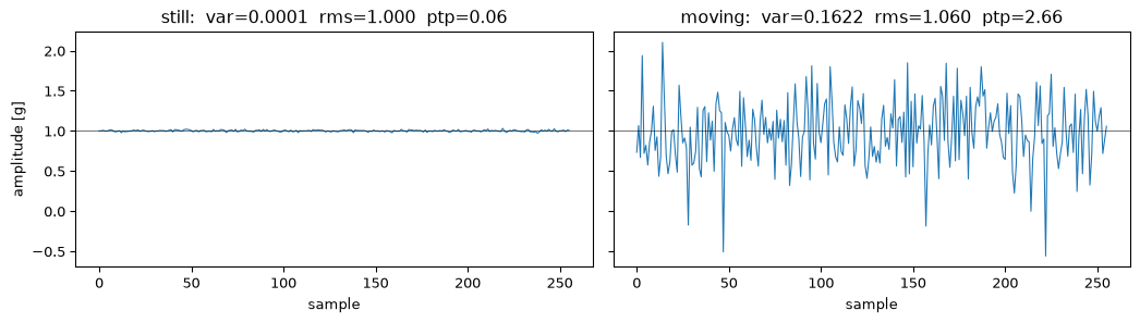
The first job of any feature set is to tell a quiet window from a busy one. Variance, RMS, energy and peak-to-peak all do it; they differ in how a lone spike sways them. Here are two windows that share the same mean but not the same activity.

Code

rng = np.random.default_rng(0)
N = 256
still  = 1.0 + 0.01 * rng.standard_normal(N)
moving = 1.0 + 0.40 * rng.standard_normal(N)

fig, axes = plt.subplots(1, 2, figsize=(11, 3.2), sharey=True)
for ax, (x, name) in zip(axes, [(still, 'still'), (moving, 'moving')]):
    ax.plot(x, 'C0', lw=0.8)
    ax.set_title(f"{name}:  var={variance(x):.4f}  rms={rms(x):.3f}  ptp={peak_to_peak(x):.2f}")
    ax.set_xlabel('sample'); ax.axhline(1.0, color='k', lw=0.4)
axes[0].set_ylabel('amplitude [g]')
fig.tight_layout(); plt.show()

ratio = variance(moving) / variance(still)
print(f"variance ratio moving/still = {ratio:.0f}x")
assert variance(moving) > 100 * variance(still)   # cleanly separable by variance
assert peak_to_peak(moving) > 10 * peak_to_peak(still)  # peak-to-peak jumps an order of magnitude too
assert rms(moving) < 1.2 * rms(still)             # but RMS barely moves: the 1 g DC offset dominates both
assert np.isclose(mean(still), mean(moving), atol=0.05)  # same level, different spread

Figure 1: A still window (tiny jitter about a 1 g offset) and a moving one (large swings about the same offset). They share a mean, and variance and peak-to-peak both jump by more than an order of magnitude, while RMS barely shifts because the 1 g DC offset dominates both windows. Variance is the single feature an activity classifier keys on.

variance ratio moving/still = 1584x

The means agree while the variance ratio is in the hundreds: spread, not level, is what tells these apart.

Shape separates signals that share a spread

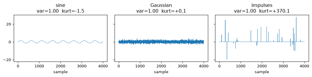
Variance is blind to how a window is distributed. Three windows can have identical variance and look completely different, and that is what the shape moments are for. The cleanest example is kurtosis sorting an oscillation, Gaussian noise, and an impulsive signal, all scaled to the same variance.

Code

rng = np.random.default_rng(1)
M = 4000
sine    = np.sin(2*np.pi*np.arange(M)*8/M)
gauss   = rng.standard_normal(M)
impulse = np.zeros(M); impulse[rng.integers(0, M, 30)] = rng.standard_normal(30)
# normalise each to unit variance so only the shape differs
sine, gauss, impulse = (z / np.std(z) for z in (sine, gauss, impulse))

fig, axes = plt.subplots(1, 3, figsize=(11, 2.8), sharey=True)
for ax, (z, name) in zip(axes, [(sine,'sine'), (gauss,'Gaussian'), (impulse,'impulses')]):
    ax.plot(z, 'C0', lw=0.6)
    ax.set_title(f"{name}\nvar={variance(z):.2f}  kurt={kurtosis(z):+.1f}")
    ax.set_xlabel('sample')
fig.tight_layout(); plt.show()

ks, kg, ki = kurtosis(sine), kurtosis(gauss), kurtosis(impulse)
print(f"excess kurtosis  sine {ks:+.2f}   Gaussian {kg:+.2f}   impulses {ki:+.1f}")
assert ks < -1.0 < kg < 1.0 < ki        # the order the caption claims, with margin
assert np.allclose([variance(sine), variance(gauss), variance(impulse)], 1.0)  # variance cannot tell them apart

Figure 2: Three windows normalised to unit variance: a sine, Gaussian noise, and a sparse impulse train. Variance cannot tell them apart, but excess kurtosis orders them cleanly, from the flat-topped sine (negative) through the Gaussian (~0) to the heavy-tailed impulses (large positive).

excess kurtosis  sine -1.50   Gaussian +0.08   impulses +370.1

Skewness is the companion: it catches asymmetry that kurtosis and variance both miss, for instance a one-sided impulse train versus a symmetric one of the same variance and tail weight.

The kurtosis mixture trap

A tempting mistake: “uniform noise is platykurtic (negative excess), so adding a uniform component lowers kurtosis.” It depends on the width. Adding a wide secondary component to a narrow one puts mass far out in the tails, so the mixture is heavy-tailed (positive excess), even though that wide component is platykurtic in isolation. Reason about the mixture, not the parts.

rng = np.random.default_rng(2)
narrow = rng.standard_normal(9000)            # sigma = 1
wide   = rng.uniform(-5, 5, size=1000)        # sigma ~ 2.9: it lands in the tails
mixture = np.concatenate([narrow, wide])
print(f"wide uniform alone: kurt={kurtosis(wide):+.2f} (platykurtic)")
print(f"narrow+wide mixture: kurt={kurtosis(mixture):+.2f} (leptokurtic!)")
assert kurtosis(wide) < 0 < kurtosis(mixture)  # the part is flat, the whole is heavy

wide uniform alone: kurt=-1.19 (platykurtic)
narrow+wide mixture: kurt=+2.15 (leptokurtic!)

Zero-crossing rate: frequency on the cheap

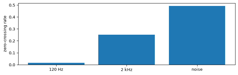
The zero-crossing rate rises with the high-frequency content of a window and ignores its amplitude entirely. That makes it a cheap brightness proxy and the classic way to separate a voiced speech sound (low ZCR, energy in the low harmonics) from an unvoiced fricative or hiss (high ZCR).

Code

t = np.arange(fs // 2) / fs
low   = np.sin(2*np.pi*120*t)
high  = np.sin(2*np.pi*2000*t)
noise = np.random.default_rng(3).standard_normal(t.size)
low, high, noise = (z / rms(z) for z in (low, high, noise))   # equal RMS

for z, name in [(low,'120 Hz tone'), (high,'2 kHz tone'), (noise,'noise')]:
    print(f"{name:12s} ZCR={zero_crossing_rate(z):.3f}  rms={rms(z):.2f}")

fig, ax = plt.subplots(figsize=(8, 2.6))
ax.bar(['120 Hz','2 kHz','noise'],
       [zero_crossing_rate(z) for z in (low, high, noise)], color='C0')
ax.set_ylabel('zero-crossing rate'); fig.tight_layout(); plt.show()

assert zero_crossing_rate(low) < zero_crossing_rate(high) < zero_crossing_rate(noise)
assert abs(rms(low) - rms(high)) < 1e-9 and abs(rms(low) - rms(noise)) < 1e-9  # all three equal RMS

120 Hz tone  ZCR=0.015  rms=1.00
2 kHz tone   ZCR=0.250  rms=1.00
noise        ZCR=0.492  rms=1.00

Figure 3: Zero-crossing rate of a low tone, a high tone, and broadband noise, all at the same RMS. ZCR tracks frequency content and is indifferent to amplitude: it rises from the low tone to the high tone to the noise.

A windowed ZCR recovers the zero-crossing chapter’s frequency estimate exactly: a rate $z$ over a window of $N$ samples at $f_s$ implies $\hat f = z\,(N-1)\cdot \frac{f_s}{2(N-1)} = \tfrac{1}{2} z f_s$.

The headline use: a fingerprint per window

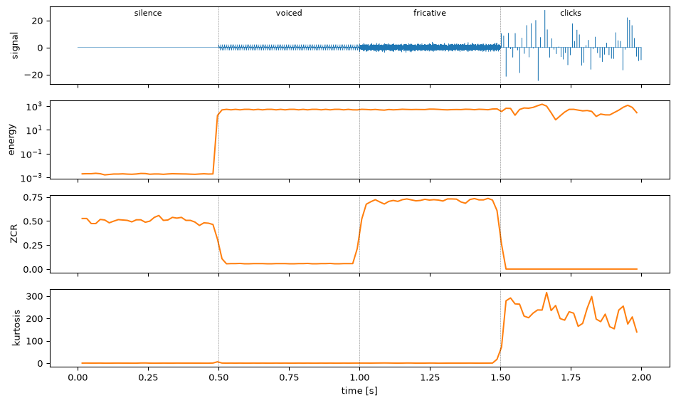
Put the features together and slide a window along a signal, and each kind of content leaves a distinct fingerprint. Here is a signal stitched from four segments, silence, a voiced sound, a noisy fricative, and a burst of impulsive clicks, with the per-window features underneath.

Code

rng = np.random.default_rng(4)
seg = fs // 2                                   # 0.5 s per segment
t = np.arange(seg) / fs

silence  = 0.002 * rng.standard_normal(seg)
voiced   = sum(np.sin(2*np.pi*k*150*t) for k in (1, 2, 3))   # three low harmonics
b, a = butter(4, 4000/(fs/2), 'high')
fricative = lfilter(b, a, rng.standard_normal(seg))
clicks = np.zeros(seg)
clicks[np.arange(60, seg, 130)] = rng.standard_normal(len(np.arange(60, seg, 130)))

segs = [silence, voiced/np.std(voiced),
        fricative/np.std(fricative), clicks/np.std(clicks)]
labels = ['silence', 'voiced', 'fricative', 'clicks']
signal = np.concatenate(segs)

win, hop = 512, 256
F = frames(signal, win, hop)
e   = energy(F); z = zero_crossing_rate(F); k = kurtosis(F)
tw  = (np.arange(F.shape[0]) * hop + win/2) / fs

fig, axes = plt.subplots(4, 1, figsize=(10, 6), sharex=True)
axes[0].plot(np.arange(signal.size)/fs, signal, 'C0', lw=0.4); axes[0].set_ylabel('signal')
for ax, v, name in zip(axes[1:], [e, z, k], ['energy','ZCR','kurtosis']):
    ax.plot(tw, v, 'C1'); ax.set_ylabel(name)
axes[1].set_yscale('log')
for ax in axes:
    for i in range(1, 4): ax.axvline(i*seg/fs, color='k', lw=0.4, ls=':')
for i, name in enumerate(labels):
    axes[0].text((i+0.5)*seg/fs, signal.max()*0.85, name, ha='center', fontsize=8)
axes[-1].set_xlabel('time [s]'); fig.tight_layout(); plt.show()

# each segment's mean feature vector, computed on its own windows
def seg_feats(x):
    Fs = frames(x, win, hop)
    return energy(Fs).mean(), zero_crossing_rate(Fs).mean(), kurtosis(Fs).mean()
fe = {name: seg_feats(x) for name, x in zip(labels, segs)}
print("segment      energy      ZCR    kurtosis")
for name in labels:
    print(f"{name:10s} {fe[name][0]:9.2f} {fe[name][1]:7.3f} {fe[name][2]:8.1f}")

assert fe['silence'][0] < 1.0 < min(fe['voiced'][0], fe['fricative'][0], fe['clicks'][0])  # energy wakes on all three
assert fe['voiced'][1] < fe['fricative'][1]             # ZCR: voiced below fricative
assert fe['clicks'][2] > 50 > max(fe['voiced'][2], fe['fricative'][2])  # kurtosis fires only on clicks

Figure 4: Top: a signal of four segments (silence, voiced harmonics, fricative noise, impulsive clicks). Below: three per-window features on the same time axis. Energy wakes on the three non-silent segments; ZCR separates the low-pitched voiced sound from the hissy fricative; kurtosis fires only on the impulsive clicks. No single feature labels all four, but together they do.

segment      energy      ZCR    kurtosis
silence         0.00   0.505     -0.0
voiced        512.00   0.056     -0.1
fricative     513.92   0.713      0.1
clicks        516.67   0.000    230.5

Read the table as the classifier does: silence is the only low-energy row, the fricative out-crosses the voiced sound, and the clicks are the only leptokurtic row. Three cheap numbers, four separable classes.

A two-feature decision rule

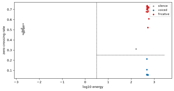
The very simplest classifier is a pair of thresholds. Log-energy against zero-crossing rate already carves audio windows into silence, voiced, and unvoiced, the textbook front end of a voice-activity gate.

Code

loge = np.log10(energy(F) + 1e-9)
zcr  = zero_crossing_rate(F)
# which segment each window centre falls in (0 silence, 1 voiced, 2 fricative)
which = np.clip(((np.arange(F.shape[0]) * hop + win/2) // seg).astype(int), 0, 3)
colors = ['0.6', 'C0', 'C3']

fig, ax = plt.subplots(figsize=(7.5, 4))
for i, name in enumerate(['silence', 'voiced', 'fricative']):  # the VAD's three classes
    m = which == i
    ax.scatter(loge[m], zcr[m], s=14, c=colors[i], label=name)
e_thresh, z_thresh = 0.5, 0.25
ax.axvline(e_thresh, color='k', ls='--', lw=0.8)
ax.plot([e_thresh, loge.max()+0.3], [z_thresh, z_thresh], 'k--', lw=0.8)
ax.set_xlabel('log10 energy'); ax.set_ylabel('zero-crossing rate')
ax.legend(fontsize=8); fig.tight_layout(); plt.show()

def classify(le, zc):
    if le < e_thresh:   return 'silence'
    return 'unvoiced' if zc > z_thresh else 'voiced'

# the rule labels each segment's median window correctly
truth = {'silence': 'silence', 'voiced': 'voiced', 'fricative': 'unvoiced'}
for i, name in enumerate(['silence', 'voiced', 'fricative']):
    m = which == i
    pred = classify(np.median(loge[m]), np.median(zcr[m]))
    print(f"{name:10s} -> {pred}")
    assert pred == truth[name]

Figure 5: Windows of the silence, voiced, and fricative segments in the (log-energy, ZCR) plane. A low-energy threshold peels off silence; among the loud windows, a ZCR threshold splits voiced (low) from unvoiced (high). Two features, three classes, two straight lines.

silence    -> silence
voiced     -> voiced
fricative  -> unvoiced

That is the whole idea of the embedded voice-activity gate: two integers per window and two comparisons, no spectrum required.

When each feature fails

The honest half of the page. Each statistic has a blind spot, and naming them is what keeps the feature set from being trusted past its range.

Mean is useless for any zero-mean signal (most audio). On an accelerometer it reports orientation, not motion, so a tilted-but-still sensor and a level-but-still one look different while both are at rest.
Variance, RMS, energy cannot tell what is loud. A loud tone and loud noise have the same variance; a louder version of a signal and a different, quieter signal can tie. Spread answers “how much”, never “what kind”.
Peak-to-peak is decided by two samples, so one spike or one clipped sample sets it. It disagrees with variance exactly when a window is impulsive, which is sometimes the tell you want and sometimes a trap.
Skewness and kurtosis are high-order moments, so they are noisy on short windows and dominated by the largest few samples. A single outlier can swing kurtosis hard. They need a few hundred samples to be stable, and they assume the window is roughly stationary.
Zero-crossing rate is fooled by additive noise (which adds spurious crossings near zero) and by DC offset (which can suppress them entirely). Mean-remove and lightly low-pass before trusting it, exactly the robustness story of the zero-crossing chapter.

The throughline: these features are cheap because they throw information away, and each one throws away something different. Use two or three with complementary blind spots, as the decision rule above does, and you cover for any one of them.

Going further

Statistical features are a floor, not a ceiling, and it is worth being clear about where they stop.

They are not time-aware within a window. Every feature here is permutation-invariant: shuffle the samples and the mean, variance, and kurtosis are unchanged (ZCR is the lone exception). Order, the very thing the STFT and autocorrelation keep, is discarded. When when matters inside the window, you need a transform.
Higher moments are fragile. Beyond kurtosis the moments are so outlier-dominated as to be unreliable on real windows; robust alternatives (median, MAD, interquartile range) trade a little efficiency for a lot of stability, and the outlier-detection page leans on exactly those.
They pair naturally with spectral features. The strong baselines in activity and audio recognition concatenate these time-domain statistics with the spectral ones and let a small classifier weigh them. The two families have largely independent blind spots, which is why the combination beats either alone.
The learned path starts here too. A deep model fed raw windows effectively rediscovers features like these in its first layers; computing them by hand is the interpretable, training-free version that runs on a coin cell. The embedded page takes that route to its conclusion.

References

Bao, Ling, and Stephen S. Intille. 2004. “Activity Recognition from User-Annotated Acceleration Data.” In Pervasive Computing (Pervasive 2004), 3001:1–17. Lecture Notes in Computer Science. Springer.

Rabiner, Lawrence R., and Biing-Hwang Juang. 1993. Fundamentals of Speech Recognition. Prentice Hall.

--- title: "Statistical Features" subtitle: "Summarising a window of samples without a transform" bibliography: ../../references.bib --- The [spectral features](../spectral-features/index.qmd) and [MFCC](../mfcc/index.qmd) pages both start by transforming a frame of audio into a spectrum and then describe *that*. This page does the cheaper thing: it describes the window of raw samples directly, with a handful of summary statistics. No FFT, no filterbank, just sums and a few powers. The result is a feature front end so cheap a microcontroller can compute it faster than the samples arrive, which is exactly why it is the workhorse of accelerometer activity recognition [@bao2004activity] and the first gate of a simple voice-activity detector [@rabiner1993fundamentals]. It is the consolidation page for the [feature-extraction track](../feature-extraction.qmd): the time-domain sibling of the spectral pages. Often these statistics are all you need; just as often they are the baseline a spectral or learned feature has to beat. The point of the page is less the formulas, which are first-year statistics, than **what each one captures and, more importantly, when each one fails to tell two signals apart**. ::: {.callout-note title="Prerequisites"} Only [signals and sampling](../../basics/01-signals.qmd) and a little [noise](../../basics/03-noise-snr.qmd). The clean, importable code is in [`statistical_features.py`](statistical_features.py), checked by [`test_statistical_features.py`](test_statistical_features.py). The zero-crossing rate is used here as one feature among several; the [zero-crossing](../../basics/zero-crossing.qmd) chapter covers it in full as a frequency estimator. The embedded companion, [the cheapest viable classifier](embedded.qmd), turns these features into an on-device activity detector and a voice gate. ::: ```{python} #| echo: false import numpy as np import matplotlib.pyplot as plt from scipy.signal import butter, lfilter from statistical_features import ( mean, variance, std, rms, energy, peak_to_peak, skewness, kurtosis, zero_crossing_rate, frame_features, ) fs = 16000 def frames(x, win, hop): """Slice a 1-D signal into a (n_windows, win) array of hopped windows.""" n = 1 + (len(x) - win) // hop idx = np.arange(win)[None, :] + hop * np.arange(n)[:, None] return x[idx] ``` ## The four families A window of $N$ samples $x[0], \dots, x[N-1]$ collapses to a few numbers. They sort into four groups by what they measure. **Level.** The mean $\mu = \frac{1}{N}\sum_n x[n]$ is the DC component: gravity on an accelerometer axis, or the (usually negligible) offset of an audio frame. It seldom discriminates *activity* on its own, but it anchors the moments below. **Spread and power.** These carry most of the "is anything happening" signal: $$\sigma^2 = \frac{1}{N}\sum_n (x[n]-\mu)^2, \qquad \text{RMS} = \sqrt{\frac{1}{N}\sum_n x[n]^2}, \qquad E = \sum_n x[n]^2$$ with peak-to-peak $\max_n x[n] - \min_n x[n]$ the cheapest amplitude measure of all. RMS and standard deviation coincide for a zero-mean window; in general $\text{RMS}^2 = \mu^2 + \sigma^2$. Energy is just $N$ times mean power, so it only compares fairly across equal-length windows. **Shape.** The third and fourth standardised moments describe the *distribution* of sample values, independent of its level and spread: $$\text{skew} = \frac{\frac{1}{N}\sum_n (x[n]-\mu)^3}{\sigma^3}, \qquad \text{kurt}_{\text{excess}} = \frac{\frac{1}{N}\sum_n (x[n]-\mu)^4}{\sigma^4} - 3$$ Skewness measures asymmetry (zero for a symmetric window, positive when the long tail is on the high side). Excess kurtosis measures tailedness: zero for a Gaussian, **positive** for a peaky, heavy-tailed window (rare large excursions: impulsive noise, transients), **negative** for a flat-topped or bounded one. The $-3$ makes the Gaussian the reference. **Oscillation.** The zero-crossing rate, the fraction of adjacent sample pairs that change sign, is a coarse, amplitude-free proxy for how much high-frequency content a window holds. It is the time-domain cousin of the [spectral centroid](../spectral-features/index.qmd) and the classic voiced/unvoiced cue in speech. ## Level and spread separate quiet from busy The first job of any feature set is to tell a quiet window from a busy one. Variance, RMS, energy and peak-to-peak all do it; they differ in how a lone spike sways them. Here are two windows that share the same mean but not the same activity. ```{python} #| label: fig-spread #| fig-cap: "A still window (tiny jitter about a 1 g offset) and a moving one (large swings about the same offset). They share a mean, and variance and peak-to-peak both jump by more than an order of magnitude, while RMS barely shifts because the 1 g DC offset dominates both windows. Variance is the single feature an activity classifier keys on." #| code-fold: true rng = np.random.default_rng(0) N = 256 still = 1.0 + 0.01 * rng.standard_normal(N) moving = 1.0 + 0.40 * rng.standard_normal(N) fig, axes = plt.subplots(1, 2, figsize=(11, 3.2), sharey=True) for ax, (x, name) in zip(axes, [(still, 'still'), (moving, 'moving')]): ax.plot(x, 'C0', lw=0.8) ax.set_title(f"{name}: var={variance(x):.4f} rms={rms(x):.3f} ptp={peak_to_peak(x):.2f}") ax.set_xlabel('sample'); ax.axhline(1.0, color='k', lw=0.4) axes[0].set_ylabel('amplitude [g]') fig.tight_layout(); plt.show() ratio = variance(moving) / variance(still) print(f"variance ratio moving/still = {ratio:.0f}x") assert variance(moving) > 100 * variance(still) # cleanly separable by variance assert peak_to_peak(moving) > 10 * peak_to_peak(still) # peak-to-peak jumps an order of magnitude too assert rms(moving) < 1.2 * rms(still) # but RMS barely moves: the 1 g DC offset dominates both assert np.isclose(mean(still), mean(moving), atol=0.05) # same level, different spread ``` The means agree while the variance ratio is in the hundreds: spread, not level, is what tells these apart. ## Shape separates signals that share a spread Variance is blind to *how* a window is distributed. Three windows can have identical variance and look completely different, and that is what the shape moments are for. The cleanest example is kurtosis sorting an oscillation, Gaussian noise, and an impulsive signal, all scaled to the same variance. ```{python} #| label: fig-shape #| fig-cap: "Three windows normalised to unit variance: a sine, Gaussian noise, and a sparse impulse train. Variance cannot tell them apart, but excess kurtosis orders them cleanly, from the flat-topped sine (negative) through the Gaussian (~0) to the heavy-tailed impulses (large positive)." #| code-fold: true rng = np.random.default_rng(1) M = 4000 sine = np.sin(2*np.pi*np.arange(M)*8/M) gauss = rng.standard_normal(M) impulse = np.zeros(M); impulse[rng.integers(0, M, 30)] = rng.standard_normal(30) # normalise each to unit variance so only the shape differs sine, gauss, impulse = (z / np.std(z) for z in (sine, gauss, impulse)) fig, axes = plt.subplots(1, 3, figsize=(11, 2.8), sharey=True) for ax, (z, name) in zip(axes, [(sine,'sine'), (gauss,'Gaussian'), (impulse,'impulses')]): ax.plot(z, 'C0', lw=0.6) ax.set_title(f"{name}\nvar={variance(z):.2f} kurt={kurtosis(z):+.1f}") ax.set_xlabel('sample') fig.tight_layout(); plt.show() ks, kg, ki = kurtosis(sine), kurtosis(gauss), kurtosis(impulse) print(f"excess kurtosis sine {ks:+.2f} Gaussian {kg:+.2f} impulses {ki:+.1f}") assert ks < -1.0 < kg < 1.0 < ki # the order the caption claims, with margin assert np.allclose([variance(sine), variance(gauss), variance(impulse)], 1.0) # variance cannot tell them apart ``` Skewness is the companion: it catches asymmetry that kurtosis and variance both miss, for instance a one-sided impulse train versus a symmetric one of the same variance and tail weight. ::: {.callout-warning title="The kurtosis mixture trap"} A tempting mistake: "uniform noise is platykurtic (negative excess), so adding a uniform component lowers kurtosis." It depends on the *width*. Adding a **wide** secondary component to a narrow one puts mass far out in the tails, so the **mixture** is heavy-tailed (positive excess), even though that wide component is platykurtic in isolation. Reason about the mixture, not the parts. ```{python} #| label: mixture-trap rng = np.random.default_rng(2) narrow = rng.standard_normal(9000) # sigma = 1 wide = rng.uniform(-5, 5, size=1000) # sigma ~ 2.9: it lands in the tails mixture = np.concatenate([narrow, wide]) print(f"wide uniform alone: kurt={kurtosis(wide):+.2f} (platykurtic)") print(f"narrow+wide mixture: kurt={kurtosis(mixture):+.2f} (leptokurtic!)") assert kurtosis(wide) < 0 < kurtosis(mixture) # the part is flat, the whole is heavy ``` ::: ## Zero-crossing rate: frequency on the cheap The zero-crossing rate rises with the high-frequency content of a window and ignores its amplitude entirely. That makes it a cheap brightness proxy and the classic way to separate a voiced speech sound (low ZCR, energy in the low harmonics) from an unvoiced fricative or hiss (high ZCR). ```{python} #| label: fig-zcr #| fig-cap: "Zero-crossing rate of a low tone, a high tone, and broadband noise, all at the same RMS. ZCR tracks frequency content and is indifferent to amplitude: it rises from the low tone to the high tone to the noise." #| code-fold: true t = np.arange(fs // 2) / fs low = np.sin(2*np.pi*120*t) high = np.sin(2*np.pi*2000*t) noise = np.random.default_rng(3).standard_normal(t.size) low, high, noise = (z / rms(z) for z in (low, high, noise)) # equal RMS for z, name in [(low,'120 Hz tone'), (high,'2 kHz tone'), (noise,'noise')]: print(f"{name:12s} ZCR={zero_crossing_rate(z):.3f} rms={rms(z):.2f}") fig, ax = plt.subplots(figsize=(8, 2.6)) ax.bar(['120 Hz','2 kHz','noise'], [zero_crossing_rate(z) for z in (low, high, noise)], color='C0') ax.set_ylabel('zero-crossing rate'); fig.tight_layout(); plt.show() assert zero_crossing_rate(low) < zero_crossing_rate(high) < zero_crossing_rate(noise) assert abs(rms(low) - rms(high)) < 1e-9 and abs(rms(low) - rms(noise)) < 1e-9 # all three equal RMS ``` A windowed ZCR recovers the [zero-crossing chapter's](../../basics/zero-crossing.qmd) frequency estimate exactly: a rate $z$ over a window of $N$ samples at $f_s$ implies $\hat f = z\,(N-1)\cdot \frac{f_s}{2(N-1)} = \tfrac{1}{2} z f_s$. ## The headline use: a fingerprint per window Put the features together and slide a window along a signal, and each kind of content leaves a distinct fingerprint. Here is a signal stitched from four segments, silence, a voiced sound, a noisy fricative, and a burst of impulsive clicks, with the per-window features underneath. ```{python} #| label: fig-fingerprint #| fig-cap: "Top: a signal of four segments (silence, voiced harmonics, fricative noise, impulsive clicks). Below: three per-window features on the same time axis. Energy wakes on the three non-silent segments; ZCR separates the low-pitched voiced sound from the hissy fricative; kurtosis fires only on the impulsive clicks. No single feature labels all four, but together they do." #| code-fold: true rng = np.random.default_rng(4) seg = fs // 2 # 0.5 s per segment t = np.arange(seg) / fs silence = 0.002 * rng.standard_normal(seg) voiced = sum(np.sin(2*np.pi*k*150*t) for k in (1, 2, 3)) # three low harmonics b, a = butter(4, 4000/(fs/2), 'high') fricative = lfilter(b, a, rng.standard_normal(seg)) clicks = np.zeros(seg) clicks[np.arange(60, seg, 130)] = rng.standard_normal(len(np.arange(60, seg, 130))) segs = [silence, voiced/np.std(voiced), fricative/np.std(fricative), clicks/np.std(clicks)] labels = ['silence', 'voiced', 'fricative', 'clicks'] signal = np.concatenate(segs) win, hop = 512, 256 F = frames(signal, win, hop) e = energy(F); z = zero_crossing_rate(F); k = kurtosis(F) tw = (np.arange(F.shape[0]) * hop + win/2) / fs fig, axes = plt.subplots(4, 1, figsize=(10, 6), sharex=True) axes[0].plot(np.arange(signal.size)/fs, signal, 'C0', lw=0.4); axes[0].set_ylabel('signal') for ax, v, name in zip(axes[1:], [e, z, k], ['energy','ZCR','kurtosis']): ax.plot(tw, v, 'C1'); ax.set_ylabel(name) axes[1].set_yscale('log') for ax in axes: for i in range(1, 4): ax.axvline(i*seg/fs, color='k', lw=0.4, ls=':') for i, name in enumerate(labels): axes[0].text((i+0.5)*seg/fs, signal.max()*0.85, name, ha='center', fontsize=8) axes[-1].set_xlabel('time [s]'); fig.tight_layout(); plt.show() # each segment's mean feature vector, computed on its own windows def seg_feats(x): Fs = frames(x, win, hop) return energy(Fs).mean(), zero_crossing_rate(Fs).mean(), kurtosis(Fs).mean() fe = {name: seg_feats(x) for name, x in zip(labels, segs)} print("segment energy ZCR kurtosis") for name in labels: print(f"{name:10s} {fe[name][0]:9.2f} {fe[name][1]:7.3f} {fe[name][2]:8.1f}") assert fe['silence'][0] < 1.0 < min(fe['voiced'][0], fe['fricative'][0], fe['clicks'][0]) # energy wakes on all three assert fe['voiced'][1] < fe['fricative'][1] # ZCR: voiced below fricative assert fe['clicks'][2] > 50 > max(fe['voiced'][2], fe['fricative'][2]) # kurtosis fires only on clicks ``` Read the table as the classifier does: silence is the only low-energy row, the fricative out-crosses the voiced sound, and the clicks are the only leptokurtic row. Three cheap numbers, four separable classes. ## A two-feature decision rule The very simplest classifier is a pair of thresholds. Log-energy against zero-crossing rate already carves audio windows into silence, voiced, and unvoiced, the textbook front end of a voice-activity gate. ```{python} #| label: fig-decision #| fig-cap: "Windows of the silence, voiced, and fricative segments in the (log-energy, ZCR) plane. A low-energy threshold peels off silence; among the loud windows, a ZCR threshold splits voiced (low) from unvoiced (high). Two features, three classes, two straight lines." #| code-fold: true loge = np.log10(energy(F) + 1e-9) zcr = zero_crossing_rate(F) # which segment each window centre falls in (0 silence, 1 voiced, 2 fricative) which = np.clip(((np.arange(F.shape[0]) * hop + win/2) // seg).astype(int), 0, 3) colors = ['0.6', 'C0', 'C3'] fig, ax = plt.subplots(figsize=(7.5, 4)) for i, name in enumerate(['silence', 'voiced', 'fricative']): # the VAD's three classes m = which == i ax.scatter(loge[m], zcr[m], s=14, c=colors[i], label=name) e_thresh, z_thresh = 0.5, 0.25 ax.axvline(e_thresh, color='k', ls='--', lw=0.8) ax.plot([e_thresh, loge.max()+0.3], [z_thresh, z_thresh], 'k--', lw=0.8) ax.set_xlabel('log10 energy'); ax.set_ylabel('zero-crossing rate') ax.legend(fontsize=8); fig.tight_layout(); plt.show() def classify(le, zc): if le < e_thresh: return 'silence' return 'unvoiced' if zc > z_thresh else 'voiced' # the rule labels each segment's median window correctly truth = {'silence': 'silence', 'voiced': 'voiced', 'fricative': 'unvoiced'} for i, name in enumerate(['silence', 'voiced', 'fricative']): m = which == i pred = classify(np.median(loge[m]), np.median(zcr[m])) print(f"{name:10s} -> {pred}") assert pred == truth[name] ``` That is the whole idea of the embedded [voice-activity gate](embedded.qmd): two integers per window and two comparisons, no spectrum required. ## When each feature fails The honest half of the page. Each statistic has a blind spot, and naming them is what keeps the feature set from being trusted past its range. - **Mean** is useless for any zero-mean signal (most audio). On an accelerometer it reports orientation, not motion, so a tilted-but-still sensor and a level-but-still one look different while both are at rest. - **Variance, RMS, energy** cannot tell *what* is loud. A loud tone and loud noise have the same variance; a louder version of a signal and a different, quieter signal can tie. Spread answers "how much", never "what kind". - **Peak-to-peak** is decided by two samples, so one spike or one clipped sample sets it. It disagrees with variance exactly when a window is impulsive, which is sometimes the tell you want and sometimes a trap. - **Skewness and kurtosis** are high-order moments, so they are noisy on short windows and dominated by the largest few samples. A single outlier can swing kurtosis hard. They need a few hundred samples to be stable, and they assume the window is roughly stationary. - **Zero-crossing rate** is fooled by additive noise (which adds spurious crossings near zero) and by DC offset (which can suppress them entirely). Mean-remove and lightly low-pass before trusting it, exactly the robustness story of the [zero-crossing chapter](../../basics/zero-crossing.qmd). The throughline: these features are cheap because they throw information away, and each one throws away something different. Use two or three with complementary blind spots, as the decision rule above does, and you cover for any one of them. ## Going further Statistical features are a floor, not a ceiling, and it is worth being clear about where they stop. - **They are not time-aware within a window.** Every feature here is permutation-invariant: shuffle the samples and the mean, variance, and kurtosis are unchanged (ZCR is the lone exception). Order, the very thing the [STFT](../stft/index.qmd) and [autocorrelation](../pitch-detection/index.qmd) keep, is discarded. When *when* matters inside the window, you need a transform. - **Higher moments are fragile.** Beyond kurtosis the moments are so outlier-dominated as to be unreliable on real windows; robust alternatives (median, MAD, interquartile range) trade a little efficiency for a lot of stability, and the [outlier-detection](../outlier-detection/index.qmd) page leans on exactly those. - **They pair naturally with spectral features.** The strong baselines in activity and audio recognition concatenate these time-domain statistics with the [spectral](../spectral-features/index.qmd) ones and let a small classifier weigh them. The two families have largely independent blind spots, which is why the combination beats either alone. - **The learned path starts here too.** A deep model fed raw windows effectively rediscovers features like these in its first layers; computing them by hand is the interpretable, training-free version that runs on a coin cell. The [embedded page](embedded.qmd) takes that route to its conclusion. ## References ::: {#refs} :::