Stochastic Resonance

When adding noise improves signal detection

A weak periodic signal sits below the threshold of a detector. No amount of linear amplification helps; the signal never crosses the threshold. Add noise. The noise occasionally pushes the signal above the threshold, and if the noise intensity is just right, the threshold crossings synchronise with the signal. The output has a higher signal-to-noise ratio than the input.

This is stochastic resonance (SR) Gammaitoni et al. (1998). It is counterintuitive, mathematically elegant, and well-established in neurobiology; less so in engineered DSP, where the Wiener or Kalman filter usually does better when the signal model is known. It earns its place in this arc as the closing argument: noise is not always the enemy.

The double-well system

The canonical SR system is an overdamped particle in a symmetric double-well potential $V(x) = -x^2/2 + x^4/4$, with a weak periodic forcing $A\cos(2\pi f_s t)$ and additive Gaussian noise $\sigma\xi(t)$:

\[\frac{dx}{dt} = x - x^3 + A\cos(2\pi f_s t) + \sigma\xi(t).\]

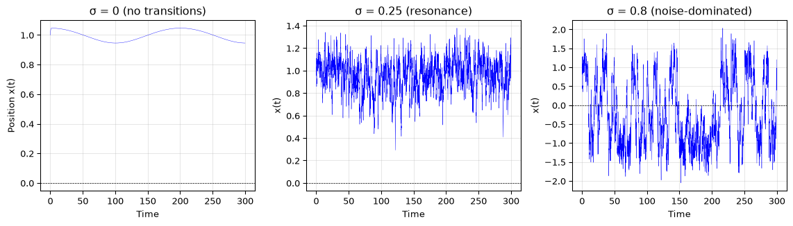
Without noise ($\sigma = 0$) and with $A < \sqrt{4/27} \approx 0.385$, the particle stays in whichever well it started in. The forcing tilts the potential back and forth, but not enough to push the particle over the barrier. Add noise and the particle occasionally hops. At the optimal noise level, the hopping rate matches the forcing frequency: the particle switches wells in sync with the signal.

n = 20000
dt = 0.1
t = np.arange(n) * dt

fig, axes = plt.subplots(1, 3, figsize=(12, 3.5))
for ax, sigma, label in zip(axes,
    [0.0, 0.25, 0.8],
    ['σ = 0 (no transitions)', 'σ = 0.25 (resonance)', 'σ = 0.8 (noise-dominated)']):
    x = double_well_system(n, A=0.1, f_sig=0.005, sigma=sigma, dt=dt, seed=42)
    ax.plot(t[:3000], x[:3000], 'b-', linewidth=0.3)
    ax.axhline(0, color='k', linestyle='--', linewidth=0.5)
    ax.set_title(label); ax.set_xlabel('Time'); ax.set_ylabel('x(t)')
    ax.grid(True, alpha=0.3)
axes[0].set_ylabel('Position x(t)')
fig.tight_layout(); plt.show()

Figure 1: Double-well system at three noise levels. Left: no noise, particle stays in one well. Center: optimal noise, hopping synchronised with the weak forcing. Right: too much noise, hopping is random, drowning the signal.

At $\sigma = 0$, the particle stays in the right well ($x > 0$). At $\sigma = 0.25$, it hops between wells, and the hopping is not random, it follows the forcing. At $\sigma = 0.8$, the hopping is dominated by the noise and the weak periodic signal is lost.

The resonance curve

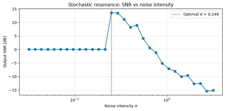
The defining signature of SR is the non-monotonic SNR-vs-noise curve. At zero noise, the SNR is zero (no transitions). As noise increases, the SNR rises to a peak at the optimal noise level. Beyond the peak, the noise dominates and the SNR falls. This is a resonance in the stochastic sense, not a frequency match but an optimal noise intensity.

sigmas = np.logspace(-1.5, 0.5, 30)
result = snr_vs_noise_curve(n=20000, A=0.1, f_sig=0.005, sigmas=sigmas, dt=0.1, seed=42)

fig, ax = plt.subplots(figsize=(8, 4))
ax.semilogx(result['sigmas'], result['snr_db'], 'C0o-', markersize=6)
ax.axvline(result['optimal_sigma'], color='C3', linestyle='--', linewidth=1,
           label=f"Optimal σ = {result['optimal_sigma']:.3f}")
ax.set_xlabel('Noise intensity σ'); ax.set_ylabel('Output SNR [dB]')
ax.set_title('Stochastic resonance: SNR vs noise intensity')
ax.legend(); ax.grid(True, alpha=0.3)
fig.tight_layout(); plt.show()
print(f"Optimal sigma: {result['optimal_sigma']:.3f}")
print(f"Peak SNR:      {result['optimal_snr_db']:.1f} dB")

Figure 2: Stochastic resonance: output SNR vs input noise intensity. The characteristic non-monotonic curve (a peak at the optimal noise level) is the signature of SR.

Optimal sigma: 0.249
Peak SNR:      13.6 dB

Biological examples

SR is not just a mathematical curiosity. It has been demonstrated in:

Crayfish mechanoreceptors (Douglass et al. 1993): hydrodynamically sensitive hairs on the crayfish tailfan detect weak water movements better in the presence of external turbulence: the turbulence provides the noise that pushes the subthreshold signal over the firing threshold.
The barn owl auditory system: the same owl from the noise whitening epigraph uses separate neural pathways for interaural time and level differences. The neurons in these pathways exhibit SR-like behaviour: adding low-level noise improves their phase-locking to weak signals.
Human balance control: standing still requires detecting small pressure changes under the feet. Adding sub-sensory mechanical noise (vibrating insoles) improves balance in elderly subjects, a clinical application of SR.

Engineered applications, and honest limits

Dither is SR in a deterministic nonlinearity: the quantiser. Adding noise before quantisation linearises the transfer function: exactly the mechanism by which noise improves detection in the double well. See the dither topic for the full treatment.

Sigma-delta conversion uses feedback to shape quantisation noise out of the signal band, but the principle (a 1-bit quantiser achieving 16-bit resolution with the help of noise) is an SR-like phenomenon.

The honest limit: SR is well-established in neurobiology but niche in engineered DSP. When you have a signal model, the Wiener or Kalman filter (see model-based filtering) is optimal and beats SR. SR’s niche is when the signal model is unknown, the detector is a hard threshold, and you can control the noise intensity, a narrow set of conditions that does arise in some sensor and biomedical applications.

Going further

Dither: SR in the quantiser, the engineered special case where the nonlinearity and the optimal noise are both known analytically.
Noise whitening: the barn owl connection.
Model-based filtering: the Wiener and Kalman filters, when you have a signal model, they beat SR.

Unlike the other topics in this arc, this page has no embedded.qmd companion: SR itself is a phenomenon, not an implementable DSP block, and its one solid engineered instance already has a hardware page: dither on hardware, where TPDF noise is generated and added before a real quantiser. If a genuinely SR-specific embedded use case emerges (per the open question below), a companion page can follow.

Open question: can SR be designed into a DSP system?

The biological examples of SR exploit noise that is already present: the crayfish does not add turbulence, it uses the turbulence that is there. An engineered SR system would need to deliberately add noise (as dither does) at a level tuned to the signal and the detector threshold. Whether this generalises beyond the quantiser to other nonlinear DSP elements (limiters, saturating amplifiers, relay-based controllers) is an open design question.

References

Benzi, Roberto, Alfonso Sutera, and Angelo Vulpiani. 1981. “The Mechanism of Stochastic Resonance.” Journal of Physics A: Mathematical and General 14 (11): L453–57.

Douglass, John K., Lon Wilkens, Eleni Pantazelou, and Frank Moss. 1993. “Noise Enhancement of Information Transfer in Crayfish Mechanoreceptors by Stochastic Resonance.” Nature 365 (6444): 337–40.

Gammaitoni, Luca, Peter Hänggi, Peter Jung, and Fabio Marchesoni. 1998. “Stochastic Resonance.” Reviews of Modern Physics 70 (1): 223–87.

--- title: "Stochastic Resonance" subtitle: "When adding noise improves signal detection" bibliography: ../../references.bib --- A weak periodic signal sits below the threshold of a detector. No amount of linear amplification helps; the signal never crosses the threshold. Add noise. The noise occasionally pushes the signal above the threshold, and if the noise intensity is *just right*, the threshold crossings synchronise with the signal. The output has a higher signal-to-noise ratio than the input. This is **stochastic resonance** (SR) [@benzi1981mechanism, @gammaitoni1998stochastic]. It is counterintuitive, mathematically elegant, and well-established in neurobiology; less so in engineered DSP, where the Wiener or Kalman filter usually does better when the signal model is known. It earns its place in this arc as the closing argument: noise is not always the enemy. ```{python} #| echo: false import numpy as np import matplotlib.pyplot as plt from stochastic_resonance import (double_well_system, threshold_crossing_detector, snr_vs_noise_curve) ``` <hr> ## The double-well system The canonical SR system is an overdamped particle in a symmetric double-well potential $V(x) = -x^2/2 + x^4/4$, with a weak periodic forcing $A\cos(2\pi f_s t)$ and additive Gaussian noise $\sigma\xi(t)$: $$\frac{dx}{dt} = x - x^3 + A\cos(2\pi f_s t) + \sigma\xi(t).$$ Without noise ($\sigma = 0$) and with $A < \sqrt{4/27} \approx 0.385$, the particle stays in whichever well it started in. The forcing tilts the potential back and forth, but not enough to push the particle over the barrier. Add noise and the particle occasionally hops. At the optimal noise level, the hopping rate matches the forcing frequency: the particle switches wells in sync with the signal. ```{python} #| label: fig-double-well #| fig-cap: "Double-well system at three noise levels. Left: no noise, particle stays in one well. Center: optimal noise, hopping synchronised with the weak forcing. Right: too much noise, hopping is random, drowning the signal." n = 20000 dt = 0.1 t = np.arange(n) * dt fig, axes = plt.subplots(1, 3, figsize=(12, 3.5)) for ax, sigma, label in zip(axes, [0.0, 0.25, 0.8], ['σ = 0 (no transitions)', 'σ = 0.25 (resonance)', 'σ = 0.8 (noise-dominated)']): x = double_well_system(n, A=0.1, f_sig=0.005, sigma=sigma, dt=dt, seed=42) ax.plot(t[:3000], x[:3000], 'b-', linewidth=0.3) ax.axhline(0, color='k', linestyle='--', linewidth=0.5) ax.set_title(label); ax.set_xlabel('Time'); ax.set_ylabel('x(t)') ax.grid(True, alpha=0.3) axes[0].set_ylabel('Position x(t)') fig.tight_layout(); plt.show() ``` At $\sigma = 0$, the particle stays in the right well ($x > 0$). At $\sigma = 0.25$, it hops between wells, and the hopping is not random, it follows the forcing. At $\sigma = 0.8$, the hopping is dominated by the noise and the weak periodic signal is lost. <hr> ## The resonance curve The defining signature of SR is the **non-monotonic SNR-vs-noise curve**. At zero noise, the SNR is zero (no transitions). As noise increases, the SNR rises to a peak at the optimal noise level. Beyond the peak, the noise dominates and the SNR falls. This is a *resonance* in the stochastic sense, not a frequency match but an optimal noise intensity. ```{python} #| label: fig-sr-curve #| fig-cap: "Stochastic resonance: output SNR vs input noise intensity. The characteristic non-monotonic curve (a peak at the optimal noise level) is the signature of SR." sigmas = np.logspace(-1.5, 0.5, 30) result = snr_vs_noise_curve(n=20000, A=0.1, f_sig=0.005, sigmas=sigmas, dt=0.1, seed=42) fig, ax = plt.subplots(figsize=(8, 4)) ax.semilogx(result['sigmas'], result['snr_db'], 'C0o-', markersize=6) ax.axvline(result['optimal_sigma'], color='C3', linestyle='--', linewidth=1, label=f"Optimal σ = {result['optimal_sigma']:.3f}") ax.set_xlabel('Noise intensity σ'); ax.set_ylabel('Output SNR [dB]') ax.set_title('Stochastic resonance: SNR vs noise intensity') ax.legend(); ax.grid(True, alpha=0.3) fig.tight_layout(); plt.show() print(f"Optimal sigma: {result['optimal_sigma']:.3f}") print(f"Peak SNR: {result['optimal_snr_db']:.1f} dB") ``` <hr> ## Biological examples SR is not just a mathematical curiosity. It has been demonstrated in: - **Crayfish mechanoreceptors** [@douglass1993noise]: hydrodynamically sensitive hairs on the crayfish tailfan detect weak water movements better in the presence of external turbulence: the turbulence provides the noise that pushes the subthreshold signal over the firing threshold. - **The barn owl auditory system**: the same owl from the [noise whitening epigraph](../noise-whitening/index.qmd) uses separate neural pathways for interaural time and level differences. The neurons in these pathways exhibit SR-like behaviour: adding low-level noise improves their phase-locking to weak signals. - **Human balance control**: standing still requires detecting small pressure changes under the feet. Adding sub-sensory mechanical noise (vibrating insoles) improves balance in elderly subjects, a clinical application of SR. <hr> ## Engineered applications, and honest limits **Dither** is SR in a deterministic nonlinearity: the quantiser. Adding noise before quantisation linearises the transfer function: exactly the mechanism by which noise improves detection in the double well. See the [dither topic](../dither/index.qmd) for the full treatment. **Sigma-delta conversion** uses feedback to shape quantisation noise out of the signal band, but the principle (a 1-bit quantiser achieving 16-bit resolution with the help of noise) is an SR-like phenomenon. **The honest limit:** SR is well-established in neurobiology but niche in engineered DSP. When you have a signal model, the Wiener or Kalman filter (see [model-based filtering](../model-based-filtering/index.qmd)) is optimal and beats SR. SR's niche is when the signal model is unknown, the detector is a hard threshold, and you can control the noise intensity, a narrow set of conditions that does arise in some sensor and biomedical applications. <hr> ## Going further - **[Dither](../dither/index.qmd)**: SR in the quantiser, the engineered special case where the nonlinearity and the optimal noise are both known analytically. - **[Noise whitening](../noise-whitening/index.qmd)**: the barn owl connection. - **[Model-based filtering](../model-based-filtering/index.qmd)**: the Wiener and Kalman filters, when you have a signal model, they beat SR. Unlike the other topics in this arc, this page has no `embedded.qmd` companion: SR itself is a phenomenon, not an implementable DSP block, and its one solid engineered instance already has a hardware page: [dither on hardware](../dither/embedded.qmd), where TPDF noise is generated and added before a real quantiser. If a genuinely SR-specific embedded use case emerges (per the open question below), a companion page can follow. ::: {.callout-warning title="Open question: can SR be designed into a DSP system?"} The biological examples of SR exploit noise that is already present: the crayfish does not add turbulence, it uses the turbulence that is there. An engineered SR system would need to deliberately add noise (as dither does) at a level tuned to the signal and the detector threshold. Whether this generalises beyond the quantiser to other nonlinear DSP elements (limiters, saturating amplifiers, relay-based controllers) is an open design question. ::: ## References ::: {#refs} :::