In 1897, physicist Amos Dolbear noticed that snowy tree crickets chirp at a rate proportional to temperature (Dolbear 1897): count the chirps in 14 seconds and add 40 to get the temperature in Fahrenheit. The cricket’s nervous system acts as a biological oscillator whose zero-crossing rate encodes environmental information. This is the same principle we use digitally to estimate frequency from sign changes.
A zero crossing is the simplest event a signal can produce: it changes sign. Despite this simplicity, zero-crossing detection is a workhorse technique in audio processing (pitch detection), vibration analysis (frequency estimation), digital communications (clock recovery), and trigger systems (oscilloscopes, data acquisition). The appeal is computational cheapness, a sign comparison and a counter, but the challenge is robustness. Noise creates false crossings, and real signals rarely cross zero cleanly.
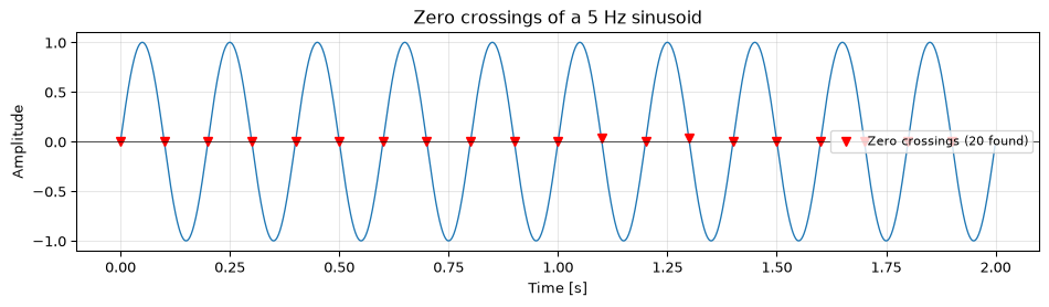
A zero crossing occurs between samples \(n\) and \(n+1\) whenever \(x[n]\) and \(x[n+1]\) have opposite signs. In practice, we detect this by checking the sign change:
import numpy as npimport matplotlib.pyplot as pltdef find_zero_crossings(x):"""Find indices where the signal crosses zero. Returns indices i where the crossing occurs between x[i] and x[i+1]. """return np.where(np.diff(np.sign(x)))[0]# Demo: clean sinusoidfs =1000t = np.arange(2000) / fsf0 =5# Hzx = np.sin(2* np.pi * f0 * t)zc = find_zero_crossings(x)#| label: fig-zero-crossings#| fig-cap: "Zero crossings of a clean sinusoid. Each sign change marks a crossing point."fig, ax = plt.subplots(figsize=(10, 3))ax.plot(t, x, 'C0', linewidth=1)ax.plot(t[zc], x[zc], 'rv', markersize=6, label=f'Zero crossings ({len(zc)} found)')ax.axhline(0, color='k', linewidth=0.5)ax.set_xlabel('Time [s]')ax.set_ylabel('Amplitude')ax.legend(fontsize=8)ax.grid(True, alpha=0.3)ax.set_title(f'Zero crossings of a {f0} Hz sinusoid')fig.tight_layout()plt.show()
For a sinusoid of frequency \(f_0\), there are two zero crossings per period (one positive-going, one negative-going), so the zero-crossing rate is \(2f_0\). This gives a simple frequency estimator:
\[\hat{f} = \frac{\text{number of zero crossings}}{2 \times \text{signal duration}}\]
Frequency estimation
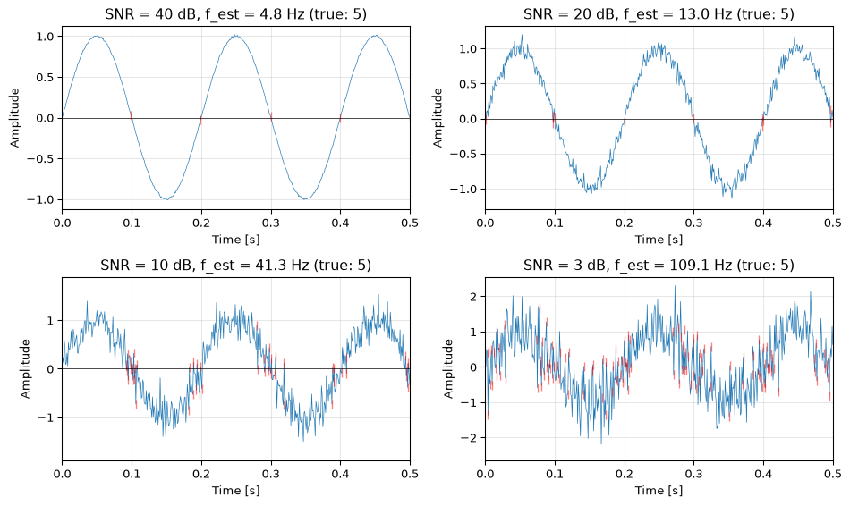
The zero-crossing frequency estimator is biased: noise increases the crossing rate (adding false crossings), so it overestimates the frequency. But for clean or well-filtered signals, it is fast and reasonably accurate.
Figure 1: Zero-crossing frequency estimation at different SNR levels. At high SNR, the estimate is accurate. As noise increases, false crossings inflate the estimate.
Hysteresis: avoiding false crossings
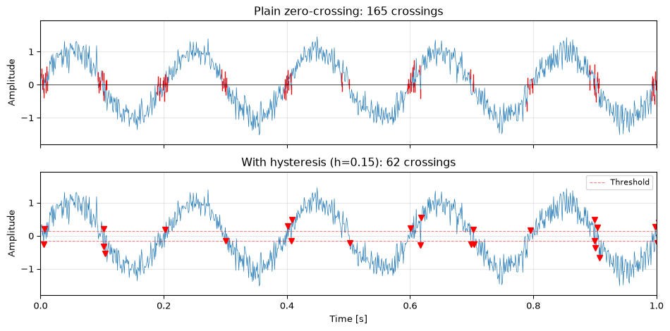
The main practical problem with zero-crossing detection is chatter: when the signal lingers near zero, noise causes rapid oscillations back and forth across the threshold, generating many spurious crossings.
The standard solution is hysteresis (also called a Schmitt trigger in hardware). Instead of a single threshold at zero, use two thresholds: an upper threshold \(+h\) and a lower threshold \(-h\). A crossing is registered only when the signal crosses the upper threshold going up (positive-going) or the lower threshold going down (negative-going). The signal must travel the full distance \(2h\) between thresholds to register a crossing, which filters out small noise excursions.
def find_crossings_hysteresis(x, threshold):"""Find zero crossings with hysteresis. Parameters ---------- x : array_like - Input signal threshold : float - Hysteresis half-width (positive value) Returns ------- crossings : ndarray - Indices of detected crossings directions : ndarray - +1 for positive-going, -1 for negative-going """ crossings = [] directions = [] state =0# 0 = indeterminate, 1 = high, -1 = low# Initialize stateif x[0] > threshold: state =1elif x[0] <-threshold: state =-1for n inrange(1, len(x)):if state ==-1and x[n] > threshold: crossings.append(n) directions.append(1) state =1elif state ==1and x[n] <-threshold: crossings.append(n) directions.append(-1) state =-1elif state ==0:if x[n] > threshold: state =1elif x[n] <-threshold: state =-1return np.array(crossings), np.array(directions)
Figure 2: Zero-crossing detection with and without hysteresis on a noisy signal. Plain detection produces many false crossings near zero; hysteresis eliminates them.
Threshold crossing (level crossing)
Zero-crossing generalises naturally to level crossing: instead of detecting where \(x[n] = 0\), detect where \(x[n] = L\) for some threshold \(L\). This is useful for trigger systems, peak detection, and event counting.
Simply subtract the level before detecting: find_zero_crossings(x - level).
For threshold-based anomaly detection, identifying when a signal exceeds a statistical boundary, see Outlier detection, which uses robust statistics (median, MAD, IQR) to set adaptive thresholds.
Sub-sample interpolation
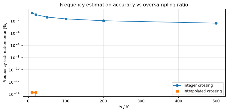
The basic detector reports the sample index before the crossing. For better timing accuracy, interpolate between the two samples straddling the crossing:
\[n_{\text{cross}} = n + \frac{|x[n]|}{|x[n]| + |x[n+1]|}\]
This linear interpolation gives sub-sample precision, which matters when the crossing rate is used for frequency estimation and the sample rate is not much higher than the signal frequency.
Figure 3: Sub-sample interpolation improves frequency estimation accuracy, especially when fs/f0 is small.
Pre-filtering
For noisy signals, the most effective strategy is to bandpass-filter the signal before counting zero crossings. The filter removes both low-frequency drift (which shifts the effective zero level) and high-frequency noise (which causes false crossings). This is standard practice in audio pitch detection and vibration frequency tracking.
The combination of bandpass filter + hysteresis + interpolation gives a robust, accurate zero-crossing detector suitable for most practical applications.
Voice pitch estimation
Zero-crossing rate (ZCR) has a long history in speech processing as a cheap proxy for both voice activity detection and pitch estimation. The idea is simple: voiced speech (vowels, nasals) is quasi-periodic, so counting zero crossings over a short frame gives a rough estimate of the fundamental frequency \(f_0\). Unvoiced sounds (fricatives like /s/, /f/) have high ZCR due to their noise-like waveform, while silence has near-zero ZCR, making it a useful feature for voiced/unvoiced/silence classification.
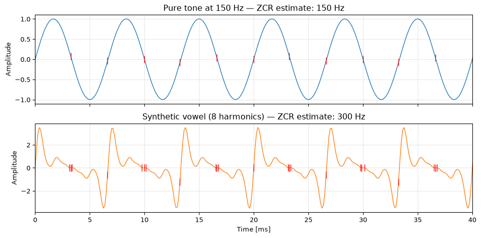
Limitations. ZCR-based pitch estimation works reliably only for signals dominated by a single frequency component. Real voiced speech is a sum of harmonics at \(f_0\), \(2f_0\), \(3f_0\), etc., and the zero crossings reflect the combined waveform rather than the fundamental. For a male voice at \(f_0 = 120\) Hz, the first three harmonics at 120, 240, and 360 Hz produce a waveform whose zero-crossing rate depends on the relative amplitudes and phases of all components, not just \(f_0\). As harmonic richness increases, ZCR increasingly overestimates the pitch.
The demo below illustrates this: a pure tone’s pitch is estimated accurately from ZCR, but a synthetic vowel (sum of harmonics) produces an inflated estimate.
import numpy as npimport matplotlib.pyplot as pltfs =8000duration =0.1# 100 ms framet = np.arange(int(fs * duration)) / fsf0 =150# Hz — typical female pitch# Pure tone at f0pure = np.sin(2* np.pi * f0 * t)# Synthetic vowel: glottal source (1/(k+1) rolloff) shaped by a formant# resonance near the 4th harmonic (~600 Hz). Real vowels have such formant# peaks; the boosted mid-harmonics add extra zero crossings, so ZCR# overestimates f0 (here it roughly doubles, reading ~300 Hz for a 150 Hz pitch).n_harmonics =8formant =4# formant resonance near the 4th harmonicamps = [(1.0/ (k +1)) * (1+3.0* np.exp(-0.5* ((k +1- formant) /1.0) **2))for k inrange(n_harmonics)]vowel =sum(a * np.sin(2* np.pi * f0 * (k +1) * t)for k, a inenumerate(amps))def zcr_frequency(x, fs):"""Estimate frequency from zero-crossing rate.""" crossings = np.where(np.diff(np.sign(x)))[0]returnlen(crossings) / (2*len(x) / fs)f_pure = zcr_frequency(pure, fs)f_vowel = zcr_frequency(vowel, fs)fig, axes = plt.subplots(2, 1, figsize=(10, 5), sharex=True)axes[0].plot(t *1000, pure, 'C0', linewidth=1)zc_pure = np.where(np.diff(np.sign(pure)))[0]axes[0].plot(t[zc_pure] *1000, pure[zc_pure], 'r|', markersize=10)axes[0].set_title(f'Pure tone at {f0} Hz — ZCR estimate: {f_pure:.0f} Hz')axes[0].set_ylabel('Amplitude')axes[1].plot(t *1000, vowel, 'C1', linewidth=1)zc_vowel = np.where(np.diff(np.sign(vowel)))[0]axes[1].plot(t[zc_vowel] *1000, vowel[zc_vowel], 'r|', markersize=10)axes[1].set_title(f'Synthetic vowel ({n_harmonics} harmonics) — ZCR estimate: {f_vowel:.0f} Hz')axes[1].set_ylabel('Amplitude')axes[1].set_xlabel('Time [ms]')for ax in axes: ax.set_xlim(0, 40) ax.grid(True, alpha=0.3)fig.tight_layout()plt.show()
Figure 4: ZCR pitch estimation for a pure tone vs a synthetic vowel. The pure tone estimate is accurate; the multi-harmonic vowel estimate is too high because upper harmonics add extra zero crossings.
For robust pitch estimation, practical systems combine ZCR with spectral methods. The VoicePitchEstimator project (ESP32-based) uses ZCR as a fast first pass for voice activity detection, then refines the pitch estimate using autocorrelation or spectral peak detection. The latter correctly identifies \(f_0\) even when upper harmonics dominate the waveform. This hybrid approach keeps computational cost low (ZCR runs continuously) while achieving the accuracy of spectral methods when it matters.
Open questions
Multi-component signals. When a signal contains multiple frequency components, the zero-crossing rate reflects a weighted combination of all components, not any single frequency. The relationship between zero-crossing rate and spectral content is given by Rice’s formula for Gaussian processes, but for arbitrary signals, the connection between zero crossings and frequency content is not straightforward. Zero-crossing analysis works best for signals dominated by a single frequency component.
Comparison with other frequency estimators. Zero-crossing frequency estimation is the simplest approach but far from the most accurate. Autocorrelation-based methods, FFT peak interpolation, and parametric methods (ESPRIT, MUSIC) all offer better resolution and noise robustness. The advantage of zero crossings is computational simplicity and suitability for hardware implementation (a comparator and a counter), which matters in embedded systems and real-time triggers.
References
Dolbear, Amos E. 1897. “The Cricket as a Thermometer.”The American Naturalist 31 (371): 970–71.
Source Code
---title: "Zero-Crossing Detection"subtitle: "Frequency and event detection from sign changes"---::: {.callout-tip title="Nature's zero-crossing detector" appearance="simple"}In 1897, physicist Amos Dolbear noticed that snowy tree crickets chirp at a rate proportional to temperature [@dolbear1897cricket]: count the chirps in 14 seconds and add 40 to get the temperature in Fahrenheit. The cricket's nervous system acts as a biological oscillator whose zero-crossing rate encodes environmental information. This is the same principle we use digitally to estimate frequency from sign changes.:::A zero crossing is the simplest event a signal can produce: it changes sign. Despite this simplicity, zero-crossing detection is a workhorse technique in audio processing (pitch detection), vibration analysis (frequency estimation), digital communications (clock recovery), and trigger systems (oscilloscopes, data acquisition). The appeal is computational cheapness, a sign comparison and a counter, but the challenge is robustness. Noise creates false crossings, and real signals rarely cross zero cleanly.::: {.callout-note title="Prerequisites"}This topic assumes familiarity with [signals and sampling](../../basics/01-signals.qmd) and [noise](../../basics/03-noise-snr.qmd). Some of the filtering strategies reference [filter design](../../basics/06-filter-design.qmd).:::---## Basic zero-crossing detectionA zero crossing occurs between samples $n$ and $n+1$ whenever $x[n]$ and $x[n+1]$ have opposite signs. In practice, we detect this by checking the sign change:```{python}import numpy as npimport matplotlib.pyplot as pltdef find_zero_crossings(x):"""Find indices where the signal crosses zero. Returns indices i where the crossing occurs between x[i] and x[i+1]. """return np.where(np.diff(np.sign(x)))[0]# Demo: clean sinusoidfs =1000t = np.arange(2000) / fsf0 =5# Hzx = np.sin(2* np.pi * f0 * t)zc = find_zero_crossings(x)#| label: fig-zero-crossings#| fig-cap: "Zero crossings of a clean sinusoid. Each sign change marks a crossing point."fig, ax = plt.subplots(figsize=(10, 3))ax.plot(t, x, 'C0', linewidth=1)ax.plot(t[zc], x[zc], 'rv', markersize=6, label=f'Zero crossings ({len(zc)} found)')ax.axhline(0, color='k', linewidth=0.5)ax.set_xlabel('Time [s]')ax.set_ylabel('Amplitude')ax.legend(fontsize=8)ax.grid(True, alpha=0.3)ax.set_title(f'Zero crossings of a {f0} Hz sinusoid')fig.tight_layout()plt.show()```For a sinusoid of frequency $f_0$, there are two zero crossings per period (one positive-going, one negative-going), so the **zero-crossing rate** is $2f_0$. This gives a simple frequency estimator:$$\hat{f} = \frac{\text{number of zero crossings}}{2 \times \text{signal duration}}$$---## Frequency estimationThe zero-crossing frequency estimator is biased: noise increases the crossing rate (adding false crossings), so it overestimates the frequency. But for clean or well-filtered signals, it is fast and reasonably accurate.```{python}#| label: fig-freq-estimation#| fig-cap: "Zero-crossing frequency estimation at different SNR levels. At high SNR, the estimate is accurate. As noise increases, false crossings inflate the estimate."rng = np.random.default_rng(42)snr_values = [40, 20, 10, 3]fig, axes = plt.subplots(2, 2, figsize=(10, 6))for ax, snr_db inzip(axes.flat, snr_values): signal_power =0.5# unit-amplitude sine has power 0.5 noise_power = signal_power *10**(-snr_db /10) x_noisy = x + np.sqrt(noise_power) * rng.standard_normal(len(x)) zc_noisy = find_zero_crossings(x_noisy) f_est =len(zc_noisy) / (2* t[-1]) ax.plot(t, x_noisy, 'C0', linewidth=0.5) ax.plot(t[zc_noisy], x_noisy[zc_noisy], 'r|', markersize=8, alpha=0.5) ax.axhline(0, color='k', linewidth=0.5) ax.set_xlabel('Time [s]') ax.set_ylabel('Amplitude') ax.set_title(f'SNR = {snr_db} dB, f_est = {f_est:.1f} Hz (true: {f0})') ax.set_xlim(0, 0.5) ax.grid(True, alpha=0.3)fig.tight_layout()plt.show()```---## Hysteresis: avoiding false crossingsThe main practical problem with zero-crossing detection is **chatter**: when the signal lingers near zero, noise causes rapid oscillations back and forth across the threshold, generating many spurious crossings.The standard solution is **hysteresis** (also called a Schmitt trigger in hardware). Instead of a single threshold at zero, use two thresholds: an upper threshold $+h$ and a lower threshold $-h$. A crossing is registered only when the signal crosses the upper threshold going up (positive-going) or the lower threshold going down (negative-going). The signal must travel the full distance $2h$ between thresholds to register a crossing, which filters out small noise excursions.```{python}def find_crossings_hysteresis(x, threshold):"""Find zero crossings with hysteresis. Parameters ---------- x : array_like - Input signal threshold : float - Hysteresis half-width (positive value) Returns ------- crossings : ndarray - Indices of detected crossings directions : ndarray - +1 for positive-going, -1 for negative-going """ crossings = [] directions = [] state =0# 0 = indeterminate, 1 = high, -1 = low# Initialize stateif x[0] > threshold: state =1elif x[0] <-threshold: state =-1for n inrange(1, len(x)):if state ==-1and x[n] > threshold: crossings.append(n) directions.append(1) state =1elif state ==1and x[n] <-threshold: crossings.append(n) directions.append(-1) state =-1elif state ==0:if x[n] > threshold: state =1elif x[n] <-threshold: state =-1return np.array(crossings), np.array(directions)``````{python}#| label: fig-hysteresis#| fig-cap: "Zero-crossing detection with and without hysteresis on a noisy signal. Plain detection produces many false crossings near zero; hysteresis eliminates them."noise_power =0.5*10**(-10/10) # 10 dB SNR (unit-amplitude sine has power 0.5)x_noisy = x + np.sqrt(noise_power) * rng.standard_normal(len(x))zc_plain = find_zero_crossings(x_noisy)zc_hyst, dirs = find_crossings_hysteresis(x_noisy, threshold=0.15)fig, axes = plt.subplots(2, 1, figsize=(10, 5), sharex=True)axes[0].plot(t, x_noisy, 'C0', linewidth=0.5)axes[0].plot(t[zc_plain], x_noisy[zc_plain], 'r|', markersize=10)axes[0].axhline(0, color='k', linewidth=0.5)axes[0].set_title(f'Plain zero-crossing: {len(zc_plain)} crossings')axes[0].set_ylabel('Amplitude')axes[1].plot(t, x_noisy, 'C0', linewidth=0.5)axes[1].plot(t[zc_hyst], x_noisy[zc_hyst], 'rv', markersize=6)axes[1].axhline(0.15, color='r', linestyle='--', linewidth=0.8, alpha=0.5, label='Threshold')axes[1].axhline(-0.15, color='r', linestyle='--', linewidth=0.8, alpha=0.5)axes[1].set_title(f'With hysteresis (h=0.15): {len(zc_hyst)} crossings')axes[1].set_xlabel('Time [s]')axes[1].set_ylabel('Amplitude')axes[1].legend(fontsize=8)for ax in axes: ax.set_xlim(0, 1) ax.grid(True, alpha=0.3)fig.tight_layout()plt.show()```---## Threshold crossing (level crossing)Zero-crossing generalises naturally to **level crossing**: instead of detecting where $x[n] = 0$, detect where $x[n] = L$ for some threshold $L$. This is useful for trigger systems, peak detection, and event counting.Simply subtract the level before detecting: `find_zero_crossings(x - level)`.For threshold-based anomaly detection, identifying when a signal exceeds a statistical boundary, see [Outlier detection](../outlier-detection/index.qmd), which uses robust statistics (median, MAD, IQR) to set adaptive thresholds.---## Sub-sample interpolationThe basic detector reports the sample index before the crossing. For better timing accuracy, interpolate between the two samples straddling the crossing:$$n_{\text{cross}} = n + \frac{|x[n]|}{|x[n]| + |x[n+1]|}$$This linear interpolation gives sub-sample precision, which matters when the crossing rate is used for frequency estimation and the sample rate is not much higher than the signal frequency.```{python}#| label: fig-interpolation#| fig-cap: "Sub-sample interpolation improves frequency estimation accuracy, especially when fs/f0 is small."# Compare integer vs interpolated zero-crossing frequency estimationf_true =5.0ratios = np.array([10, 20, 50, 100, 200, 500])errors_int = []errors_interp = []for ratio in ratios: fs_test = f_true * ratio t_test = np.arange(int(fs_test *10)) / fs_test # 10 seconds x_test = np.sin(2* np.pi * f_true * t_test)# Integer crossings zc = find_zero_crossings(x_test) f_int =len(zc) / (2* t_test[-1])# Interpolated crossings zc_interp = zc + np.abs(x_test[zc]) / (np.abs(x_test[zc]) + np.abs(x_test[zc +1])) periods = np.diff(zc_interp) / fs_test /0.5# half-periods f_interp =1.0/ np.mean(periods) iflen(periods) >0else0 errors_int.append(abs(f_int - f_true) / f_true *100) errors_interp.append(abs(f_interp - f_true) / f_true *100)fig, ax = plt.subplots(figsize=(8, 4))ax.semilogy(ratios, errors_int, 'o-', label='Integer crossing')ax.semilogy(ratios, errors_interp, 's-', label='Interpolated crossing')ax.set_xlabel('fs / f0')ax.set_ylabel('Frequency estimation error [%]')ax.legend(fontsize=9)ax.grid(True, alpha=0.3)ax.set_title('Frequency estimation accuracy vs oversampling ratio')fig.tight_layout()plt.show()```---## Pre-filteringFor noisy signals, the most effective strategy is to bandpass-filter the signal before counting zero crossings. The filter removes both low-frequency drift (which shifts the effective zero level) and high-frequency noise (which causes false crossings). This is standard practice in audio pitch detection and vibration frequency tracking.The combination of **bandpass filter + hysteresis + interpolation** gives a robust, accurate zero-crossing detector suitable for most practical applications.---## Voice pitch estimationZero-crossing rate (ZCR) has a long history in speech processing as a cheap proxy for both **voice activity detection** and **pitch estimation**. The idea is simple: voiced speech (vowels, nasals) is quasi-periodic, so counting zero crossings over a short frame gives a rough estimate of the fundamental frequency $f_0$. Unvoiced sounds (fricatives like /s/, /f/) have high ZCR due to their noise-like waveform, while silence has near-zero ZCR, making it a useful feature for voiced/unvoiced/silence classification.**Limitations.** ZCR-based pitch estimation works reliably only for signals dominated by a single frequency component. Real voiced speech is a sum of harmonics at $f_0$, $2f_0$, $3f_0$, etc., and the zero crossings reflect the combined waveform rather than the fundamental. For a male voice at $f_0 = 120$ Hz, the first three harmonics at 120, 240, and 360 Hz produce a waveform whose zero-crossing rate depends on the relative amplitudes and phases of all components, not just $f_0$. As harmonic richness increases, ZCR increasingly overestimates the pitch.The demo below illustrates this: a pure tone's pitch is estimated accurately from ZCR, but a synthetic vowel (sum of harmonics) produces an inflated estimate.```{python}#| label: fig-pitch-zcr#| fig-cap: "ZCR pitch estimation for a pure tone vs a synthetic vowel. The pure tone estimate is accurate; the multi-harmonic vowel estimate is too high because upper harmonics add extra zero crossings."import numpy as npimport matplotlib.pyplot as pltfs =8000duration =0.1# 100 ms framet = np.arange(int(fs * duration)) / fsf0 =150# Hz — typical female pitch# Pure tone at f0pure = np.sin(2* np.pi * f0 * t)# Synthetic vowel: glottal source (1/(k+1) rolloff) shaped by a formant# resonance near the 4th harmonic (~600 Hz). Real vowels have such formant# peaks; the boosted mid-harmonics add extra zero crossings, so ZCR# overestimates f0 (here it roughly doubles, reading ~300 Hz for a 150 Hz pitch).n_harmonics =8formant =4# formant resonance near the 4th harmonicamps = [(1.0/ (k +1)) * (1+3.0* np.exp(-0.5* ((k +1- formant) /1.0) **2))for k inrange(n_harmonics)]vowel =sum(a * np.sin(2* np.pi * f0 * (k +1) * t)for k, a inenumerate(amps))def zcr_frequency(x, fs):"""Estimate frequency from zero-crossing rate.""" crossings = np.where(np.diff(np.sign(x)))[0]returnlen(crossings) / (2*len(x) / fs)f_pure = zcr_frequency(pure, fs)f_vowel = zcr_frequency(vowel, fs)fig, axes = plt.subplots(2, 1, figsize=(10, 5), sharex=True)axes[0].plot(t *1000, pure, 'C0', linewidth=1)zc_pure = np.where(np.diff(np.sign(pure)))[0]axes[0].plot(t[zc_pure] *1000, pure[zc_pure], 'r|', markersize=10)axes[0].set_title(f'Pure tone at {f0} Hz — ZCR estimate: {f_pure:.0f} Hz')axes[0].set_ylabel('Amplitude')axes[1].plot(t *1000, vowel, 'C1', linewidth=1)zc_vowel = np.where(np.diff(np.sign(vowel)))[0]axes[1].plot(t[zc_vowel] *1000, vowel[zc_vowel], 'r|', markersize=10)axes[1].set_title(f'Synthetic vowel ({n_harmonics} harmonics) — ZCR estimate: {f_vowel:.0f} Hz')axes[1].set_ylabel('Amplitude')axes[1].set_xlabel('Time [ms]')for ax in axes: ax.set_xlim(0, 40) ax.grid(True, alpha=0.3)fig.tight_layout()plt.show()```For robust pitch estimation, practical systems combine ZCR with spectral methods. The VoicePitchEstimator project (ESP32-based) uses ZCR as a fast first pass for voice activity detection, then refines the pitch estimate using autocorrelation or spectral peak detection. The latter correctly identifies $f_0$ even when upper harmonics dominate the waveform. This hybrid approach keeps computational cost low (ZCR runs continuously) while achieving the accuracy of spectral methods when it matters.---## Open questions**Multi-component signals.** When a signal contains multiple frequency components, the zero-crossing rate reflects a weighted combination of all components, not any single frequency. The relationship between zero-crossing rate and spectral content is given by Rice's formula for Gaussian processes, but for arbitrary signals, the connection between zero crossings and frequency content is not straightforward. Zero-crossing analysis works best for signals dominated by a single frequency component.**Comparison with other frequency estimators.** Zero-crossing frequency estimation is the simplest approach but far from the most accurate. Autocorrelation-based methods, FFT peak interpolation, and parametric methods (ESPRIT, MUSIC) all offer better resolution and noise robustness. The advantage of zero crossings is computational simplicity and suitability for hardware implementation (a comparator and a counter), which matters in embedded systems and real-time triggers.## References::: {#refs}:::