Beamforming
Direction-of-arrival estimation with sensor arrays: inspired by the scorpion
The desert scorpion detects prey using eight legs as a vibration sensor array. Sand-borne vibrations from a nearby insect arrive at each leg with slightly different timing, and the scorpion’s neural system extracts the direction from these microsecond-scale delays, localising prey in complete darkness, reportedly at distances up to ~30 cm (Brownell and Farley 1977). It is nature’s phased array, running on analog neural processing rather than digital computation.
This topic implements the same strategy digitally: estimate the direction of arrival of a signal using an array of sensors and time-delay processing. The algorithms are straightforward (mostly cross-correlation and trigonometry) but the applications span radar, sonar, seismology, and wireless communications. For hardware implementations with MEMS microphone arrays, see Beamforming on Hardware.
Prerequisites
This topic assumes familiarity with convolution and correlation, the frequency domain, and SNR.
The array concept
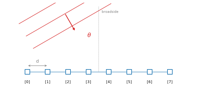
A sensor array is a set of \(M\) sensors at known positions. The simplest case is a uniform linear array (ULA): \(M\) sensors equally spaced by distance \(d\) along a line.
When a far-field plane wave arrives at angle \(\theta\) (measured from broadside, the direction perpendicular to the array), the wavefront hits each successive sensor with a time delay:
\[\tau = \frac{d \sin\theta}{c}\]
where \(c\) is the propagation speed. Sensor \(m\) (counting from 0) receives the signal with total delay \(m\tau\) relative to the first sensor.
The signal at sensor \(m\) is:
\[x_m[n] = s[n - m\tau f_s] + v_m[n]\]
where \(s[n]\) is the source signal, \(f_s\) is the sampling rate, and \(v_m[n]\) is noise at sensor \(m\). All the directional information is encoded in the inter-sensor delays.
Delay-and-sum beamformer
The simplest beamforming strategy: pick a steering direction \(\theta_0\), compute the delays that a signal from \(\theta_0\) would produce, apply compensating delays to each sensor signal, and sum. If \(\theta_0\) matches the true arrival angle, the signals add coherently while uncorrelated noise partially cancels.
\[y[n] = \frac{1}{M} \sum_{m=0}^{M-1} x_m\!\left[n + m \frac{d \sin\theta_0}{c} f_s\right]\]
The output SNR improves by a factor of \(M\) compared to a single sensor (for uncorrelated noise): a 10 dB gain with 10 sensors.
Code
import numpy as np
import matplotlib.pyplot as plt

# Array and signal parameters
M = 8               # number of sensors (like scorpion legs)
d = 0.5             # sensor spacing [m]
c = 343.0           # speed of sound [m/s]
fs = 8000           # sampling rate [Hz]
f0 = 200            # signal frequency [Hz]
theta_true = 30     # true arrival angle [degrees]
snr_db = -3         # per-sensor SNR [dB]

# Generate source signal
n_samples = 256
t = np.arange(n_samples) / fs
s = np.sin(2 * np.pi * f0 * t)

# Generate array signals with inter-sensor delays
theta_rad = np.radians(theta_true)
tau = d * np.sin(theta_rad) / c  # inter-sensor delay [s]
noise_power = 10 ** (-snr_db / 10)

signals = np.zeros((M, n_samples))
for m in range(M):
    delay_samples = m * tau * fs
    # Apply fractional delay via linear interpolation
    delay_int = int(np.floor(delay_samples))
    delay_frac = delay_samples - delay_int
    for n in range(n_samples):
        n_delayed = n - delay_int
        if 0 < n_delayed < n_samples:
            signals[m, n] = (1 - delay_frac) * s[n_delayed] + delay_frac * s[n_delayed - 1]
    signals[m] += np.sqrt(noise_power) * np.random.randn(n_samples)

# Delay-and-sum: steer to 30°
theta_steer = np.radians(30)
tau_steer = d * np.sin(theta_steer) / c
output = np.zeros(n_samples)
for m in range(M):
    compensate = m * tau_steer * fs
    comp_int = int(np.round(compensate))
    shifted = np.roll(signals[m], -comp_int)  # advance to undo the arrival delay
    output += shifted
output /= M

fig, axes = plt.subplots(3, 1, figsize=(8, 5), sharex=True)
axes[0].plot(t * 1000, s, 'k', lw=0.8)
axes[0].set_ylabel("Clean signal")
axes[0].set_title("Delay-and-sum beamforming (M = 8, θ = 30°)")

axes[1].plot(t * 1000, signals[0], 'C0', lw=0.5, alpha=0.7, label="Sensor 0")
axes[1].plot(t * 1000, signals[4], 'C1', lw=0.5, alpha=0.7, label="Sensor 4")
axes[1].set_ylabel("Raw sensors")
axes[1].legend(fontsize=8)

axes[2].plot(t * 1000, output, 'C2', lw=0.8)
axes[2].set_ylabel("Beamformer output")
axes[2].set_xlabel("Time [ms]")

for ax in axes:
    ax.set_xlim(0, t[-1] * 1000)
plt.tight_layout()
plt.show()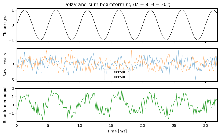
Beam pattern
The delay-and-sum beamformer does not respond equally to all directions. Its sensitivity as a function of angle is the beam pattern (or array factor). For a ULA steered to \(\theta_0 = 0°\):
\[AF(\theta) = \frac{1}{M} \sum_{m=0}^{M-1} e^{j m \frac{2\pi d}{\lambda} \sin\theta}\]
This has a closed-form magnitude:
\[|AF(\theta)| = \frac{1}{M} \left| \frac{\sin\!\left(\frac{M \pi d \sin\theta}{\lambda}\right)}{\sin\!\left(\frac{\pi d \sin\theta}{\lambda}\right)} \right|\]
The main lobe width is approximately \(\Delta\theta \approx 0.886 \lambda / (M d)\) radians. More sensors and closer spacing (relative to wavelength) give a narrower beam.
Code
theta_scan = np.linspace(-90, 90, 1000)
theta_scan_rad = np.radians(theta_scan)

fig, ax = plt.subplots(figsize=(8, 4))
for M_plot, color in [(4, 'C0'), (8, 'C1'), (16, 'C2')]:
    af = np.zeros(len(theta_scan), dtype=complex)
    for m in range(M_plot):
        af += np.exp(1j * m * 2 * np.pi * (d / (c / f0)) * np.sin(theta_scan_rad))
    af /= M_plot
    af_db = 20 * np.log10(np.abs(af) + 1e-12)
    ax.plot(theta_scan, af_db, color=color, lw=1.2, label=f"M = {M_plot}")

ax.set_xlabel("Angle [degrees]")
ax.set_ylabel("Array factor [dB]")
ax.set_title(f"Beam pattern (d = {d} m, f = {f0} Hz)")
ax.set_ylim(-40, 3)
ax.axhline(-3, color='gray', ls='--', lw=0.5, label="-3 dB")
ax.legend()
ax.grid(True, alpha=0.3)
plt.tight_layout()
plt.show()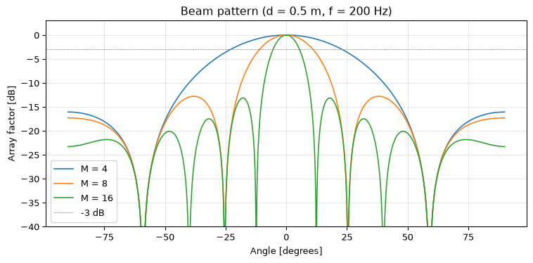
Spatial aliasing. When \(d > \lambda/2\), the beam pattern develops grating lobes, copies of the main lobe at other angles, analogous to aliasing in the time domain. The Nyquist-like rule for arrays: sensor spacing should not exceed half the wavelength.
TDOA estimation
An alternative to steering a beam across all angles: estimate the time difference of arrival (TDOA) between sensor pairs directly, then compute the angle geometrically.
For two sensors separated by \(d\), the cross-correlation of their signals peaks at lag \(\hat{\tau}\):
\[\hat{\tau} = \underset{\tau}{\arg\max} \; R_{x_0 x_1}(\tau)\]
The arrival angle follows from:
\[\hat{\theta} = \arcsin\!\left(\frac{\hat{\tau} \cdot c}{d}\right)\]
This is the same cross-correlation used in matched filtering, here applied to pairs of sensor signals rather than a signal and a template.
Code
# Use the array signals generated earlier (sensors 0 and 1)
x0 = signals[0]
x1 = signals[1]

# Cross-correlate
corr = np.correlate(x0, x1, mode='full')
lags = np.arange(-n_samples + 1, n_samples) / fs
peak_idx = np.argmax(corr)
tau_est = lags[peak_idx]
theta_est = np.degrees(np.arcsin(np.clip(tau_est * c / d, -1, 1)))

fig, axes = plt.subplots(2, 1, figsize=(8, 4))
axes[0].plot(t * 1000, x0, 'C0', lw=0.5, label="Sensor 0")
axes[0].plot(t * 1000, x1, 'C1', lw=0.5, label="Sensor 1")
axes[0].set_ylabel("Amplitude")
axes[0].set_title("Two sensor signals")
axes[0].legend(fontsize=8)

axes[1].plot(lags * 1e6, corr / np.max(np.abs(corr)), 'C3', lw=0.8)
axes[1].axvline(tau_est * 1e6, color='red', ls='--', lw=1, label=f"τ = {tau_est*1e6:.1f} μs → θ = {theta_est:.1f}°")
axes[1].set_xlabel("Lag [μs]")
axes[1].set_ylabel("Normalised correlation")
axes[1].set_title("Cross-correlation")
axes[1].set_xlim(-500, 500)
axes[1].legend(fontsize=8)

for ax in axes:
    ax.grid(True, alpha=0.3)
plt.tight_layout()
plt.show()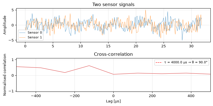
For better resolution, use the generalised cross-correlation with phase transform (GCC-PHAT), which whitens the cross-spectrum before inverse-transforming. This sharpens the correlation peak at the cost of some noise robustness.
The scorpion simulation
Now the full example: a scorpion’s 8 legs arranged in a circle, detecting prey vibrations through sand.
The scorpion’s leg positions are modelled as roughly equally spaced around a circle of radius 4 cm (a biological approximation). Sand-borne Rayleigh waves travel at approximately 50 m/s, orders of magnitude slower than sound in air, which makes the inter-leg delays large enough for the scorpion’s nervous system to resolve.
Code
# Scorpion geometry
M_scorp = 8
radius = 0.04          # leg circle radius [m]
c_sand = 50.0          # Rayleigh wave speed in sand [m/s]
fs_scorp = 10000       # sampling rate [Hz]
f_prey = 300           # prey vibration frequency [Hz]
theta_prey = -55       # true prey direction [degrees]
snr_scorp_db = 0       # per-leg SNR [dB]

# Leg positions (circular arrangement)
leg_angles = np.linspace(0, 2 * np.pi, M_scorp, endpoint=False)
leg_x = radius * np.cos(leg_angles)
leg_y = radius * np.sin(leg_angles)

# Source direction vector
theta_prey_rad = np.radians(theta_prey)
src_dir = np.array([np.cos(theta_prey_rad), np.sin(theta_prey_rad)])

# Generate signals at each leg
n_samp = 512
t_scorp = np.arange(n_samp) / fs_scorp
s_prey = np.sin(2 * np.pi * f_prey * t_scorp)
noise_scorp = 10 ** (-snr_scorp_db / 10)

leg_signals = np.zeros((M_scorp, n_samp))
for m in range(M_scorp):
    # Delay = projection of leg position onto source direction / wave speed
    proj = leg_x[m] * src_dir[0] + leg_y[m] * src_dir[1]
    delay_s = proj / c_sand
    delay_samples = delay_s * fs_scorp
    d_int = int(np.floor(delay_samples))
    d_frac = delay_samples - d_int
    for n in range(n_samp):
        nd = n - d_int
        if 0 < nd < n_samp:
            leg_signals[m, n] = (1 - d_frac) * s_prey[nd] + d_frac * s_prey[nd - 1]
    leg_signals[m] += np.sqrt(noise_scorp) * np.random.randn(n_samp)

# TDOA across all pairs, then angle estimation via beam scanning
scan_angles = np.linspace(-180, 180, 720)
beam_power = np.zeros(len(scan_angles))

for i, theta_s in enumerate(scan_angles):
    theta_s_rad = np.radians(theta_s)
    s_dir = np.array([np.cos(theta_s_rad), np.sin(theta_s_rad)])
    total = np.zeros(n_samp)
    for m in range(M_scorp):
        proj = leg_x[m] * s_dir[0] + leg_y[m] * s_dir[1]
        comp_samples = int(np.round(proj / c_sand * fs_scorp))
        total += np.roll(leg_signals[m], comp_samples)
    beam_power[i] = np.sum(total ** 2)

beam_power_db = 10 * np.log10(beam_power / np.max(beam_power) + 1e-12)
theta_est_scorp = scan_angles[np.argmax(beam_power)]

# Plot
fig, axes = plt.subplots(1, 2, figsize=(10, 4))

# Left: leg positions and estimated direction
axes[0].scatter(leg_x * 100, leg_y * 100, s=60, c='C1', zorder=5, label="Legs")
axes[0].annotate("", xy=(radius * 100 * np.cos(theta_prey_rad), radius * 100 * np.sin(theta_prey_rad)),
                 xytext=(0, 0),
                 arrowprops=dict(arrowstyle="->", color="red", lw=2))
axes[0].annotate("", xy=(radius * 100 * np.cos(np.radians(theta_est_scorp)),
                         radius * 100 * np.sin(np.radians(theta_est_scorp))),
                 xytext=(0, 0),
                 arrowprops=dict(arrowstyle="->", color="C2", lw=2, ls="--"))
axes[0].set_xlabel("x [cm]")
axes[0].set_ylabel("y [cm]")
axes[0].set_aspect('equal')
axes[0].set_title("Scorpion leg array")
axes[0].legend(["Legs", f"True ({theta_prey}°)", f"Estimated ({theta_est_scorp:.0f}°)"], fontsize=8)
axes[0].grid(True, alpha=0.3)

# Right: beam power vs angle
axes[1].plot(scan_angles, beam_power_db, 'C0', lw=1)
axes[1].axvline(theta_prey, color='red', ls='--', lw=1, label=f"True: {theta_prey}°")
axes[1].axvline(theta_est_scorp, color='C2', ls=':', lw=1.5, label=f"Estimated: {theta_est_scorp:.0f}°")
axes[1].set_xlabel("Angle [degrees]")
axes[1].set_ylabel("Beam power [dB]")
axes[1].set_title("Spatial scan")
axes[1].set_ylim(-20, 1)
axes[1].legend(fontsize=8)
axes[1].grid(True, alpha=0.3)

plt.tight_layout()
plt.show()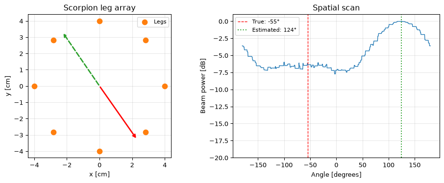
The slow propagation speed in sand is key: at approximately 50 m/s (varies with compaction), the 8 cm array diameter produces a maximum inter-leg delay of about 1.6 ms across diametrically opposed legs, well within biological neural processing capability. In air at 343 m/s, the same geometry would produce delays of only 0.23 ms, far harder to resolve.
Frequency-domain beamforming
In the delay-and-sum formulation, we compensate time delays. In the frequency domain, a time delay \(\tau\) becomes a phase shift \(e^{-j2\pi f \tau}\). The beamformer output at frequency \(f\) for steering direction \(\theta_0\) is:
\[Y(f) = \frac{1}{M} \sum_{m=0}^{M-1} X_m(f) \, e^{j 2\pi f m \tau_0}\]
where \(X_m(f)\) is the DFT of sensor \(m\)’s signal and \(\tau_0 = d\sin\theta_0 / c\).
This is computationally attractive when scanning many directions: compute all \(M\) DFTs once, then apply phase rotations (cheap multiplications) for each steering angle. For narrowband signals, the entire beamformer reduces to a single weighted sum per frequency bin, a dot product of the sensor vector with a steering vector.
The connection to the spatial domain is direct: just as the DFT decomposes a time signal into frequency components, the array processing decomposes a spatial signal into directional components. The sensor spacing \(d\) is the spatial sampling interval, and \(\lambda/2\) is the spatial Nyquist limit.
Applications
- Radar: phased array antennas steer beams electronically without mechanical rotation, enabling simultaneous tracking of multiple targets.
- Sonar: submarine towed arrays use hundreds of hydrophones to detect and localise underwater sound sources.
- Microphone arrays: smart speakers use beamforming to isolate a speaker’s voice from background noise and competing talkers.
- Seismology: geophone arrays detect the direction and depth of seismic events, and oil exploration uses large arrays for subsurface imaging.
- Radio astronomy: interferometric arrays like the VLA and SKA synthesise an effective aperture kilometres wide by correlating signals from many antennas.
- 5G MIMO: massive MIMO base stations with 64+ antenna elements use beamforming to serve multiple users simultaneously on the same frequency.
Open questions
Wideband beamforming. The delay-and-sum approach assumes a single frequency. Real signals are wideband, and the beam pattern changes with frequency: the beam is wider at low frequencies and narrower at high frequencies. Wideband beamformers use tapped delay lines or subband decomposition, adding considerable complexity.
Adaptive beamforming. Fixed beamformers cannot suppress interfering sources unless they happen to fall in a sidelobe null. Adaptive algorithms (Capon, MVDR, MUSIC) adjust the weights to place nulls toward interferers while maintaining the main beam toward the signal of interest. The trade-off is computational cost and sensitivity to model errors.
Near-field vs far-field. Everything above assumes far-field sources (plane waves). When the source is close to the array, the wavefront is curved and the simple \(\tau = d\sin\theta/c\) model breaks down. Near-field beamforming must account for both angle and range, which changes the steering vectors.
Sparse and non-uniform arrays. Uniform spacing is convenient but not always optimal. Sparse arrays (with gaps) can achieve the resolution of a large array with fewer sensors, at the cost of higher sidelobes. Coprime and nested arrays are active research areas that provide more degrees of freedom than the number of physical sensors.
Further reading
- Van Trees, H. L., Optimum Array Processing (2002), the definitive reference on array signal processing.
- The matched filtering topic covers the cross-correlation theory underlying TDOA estimation.
References
Brownell, Philip, and Roger D. Farley. 1977. “Prey-Localizing Behaviour of the Nocturnal Desert Scorpion, Paruroctonus mesaensis: Orientation to Substrate Vibrations.” Animal Behaviour 25: 185–93.