Detecting known signals in noise: from bat echolocation to gravitational waves
In 2015, the LIGO observatory detected a gravitational wave from two colliding black holes 1.3 billion light-years away. The signal was so faint that it was buried far below the noise floor. How did they find it? They correlated the measured data against a bank of 250,000 template waveforms, one for each possible combination of black hole masses and spins. The template that produced the largest correlation peak was the detection. This technique is called matched filtering, and it is provably optimal: no other linear filter can achieve a higher output signal-to-noise ratio.
The same principle explains how bats navigate in complete darkness. A bat emits a frequency-modulated chirp and listens for echoes. Its auditory system performs something functionally equivalent to matched filtering (correlating the returning sound with the expected chirp shape) to achieve the extraordinary range resolution needed to catch insects mid-flight.
Radar, sonar, GPS, wireless communications, and medical ultrasound all use the same idea. The matched filter is one of the most widely deployed algorithms in signal processing.
You know the shape of the signal you are looking for (the template), but not when it arrives or whether it is present. The received signal is:
\[r[n] = \alpha \cdot s[n - n_0] + v[n]\]
where \(s[n]\) is the known template, \(\alpha\) is an unknown amplitude, \(n_0\) is the unknown arrival time, and \(v[n]\) is additive noise. The goal is to find \(n_0\) (and decide whether the signal is present at all).
Derivation: maximising output SNR
We want a filter \(h[n]\) of length \(N\) that maximises the peak output SNR, the ratio of the peak signal power at the output to the average noise power at the output.
The filter output is:
\[y[n] = \sum_{k=0}^{N-1} h[k] \, r[n-k]\]
At the moment the template is aligned (\(n = n_0 + N - 1\)), the signal component of the output is:
By the Cauchy–Schwarz inequality, \((\mathbf{h}^T \mathbf{s}_\text{rev})^2 \leq \|\mathbf{h}\|^2 \|\mathbf{s}_\text{rev}\|^2\), with equality when \(\mathbf{h} = c \cdot \mathbf{s}_\text{rev}\) for any constant \(c\). Therefore, the filter that maximises output SNR is:
\[\boxed{h[n] = s[N-1-n]}\]
The optimal filter is the time-reversed template. Filtering with \(h[n]\) is equivalent to computing the cross-correlation of the received signal with the template.
where \(E_s\) is the template energy. The output SNR depends only on the total energy of the template, not on its shape: a longer or louder signal gives better detection regardless of waveform.
This is the cross-correlation of \(r\) with \(s\). In many implementations, matched filtering is computed as correlation rather than convolution: the two are identical when the filter is the time-reversed template.
In the frequency domain:
\[Y(f) = S^*(f) \cdot R(f)\]
where \(S^*\) is the complex conjugate of the template’s spectrum. This leads to efficient FFT-based implementations for long signals.
Pulse compression
A remarkable consequence: you can transmit a long, low-power signal and achieve the same detection performance as a short, high-power pulse. The matched filter compresses the extended signal into a sharp peak at the output.
The compression ratio is approximately equal to the time-bandwidth product:
\[\text{CR} \approx B \cdot T\]
where \(B\) is the signal bandwidth and \(T\) is its duration. A chirp sweeping 70 kHz in 2 ms has \(\text{CR} \approx 140\): the matched filter output peak is 140 times narrower than the original signal.
This is why bats use chirps rather than clicks: a chirp spreads the same energy over a longer time (keeping the instantaneous power within biological limits) while the auditory system’s correlation processing recovers the range resolution of a much shorter pulse.
Processing gain
Pulse compression buys SNR, not just resolution. The derivation above gave the peak output SNR as \(\alpha^2 E_s / \sigma_v^2\): every sample of the template adds coherently at the alignment instant while the noise adds incoherently, so a longer, wider chirp wins on both counts. Expressed as a gain of output SNR over input SNR, this processing gain is approximately the same time-bandwidth product:
\[G \approx B \cdot T\]
The front-page bat figure uses an FM chirp sweeping \(B = 55\) kHz over \(T = 4\) ms, so \(B \cdot T = 220\), a predicted gain of \(10 \log_{10}(220) \approx 23\) dB. This is real, not a plotting trick: a Monte-Carlo simulation of that exact chirp (echo amplitude 0.5 in unit-variance noise, 400 trials) measures a mean gain of 23.5 dB when the input SNR is referenced to the signal band \(B\), within rounding of the prediction. That is the whole story of the landing-page demo: an echo sitting near \(-4\) dB in the raw trace becomes a peak roughly 20 dB above the noise floor.
What ‘gain’ means here
The exact dB figure depends on how you define the input SNR. Referenced to the signal band \(B\), the gain is \(\approx B \cdot T\) (above). Referenced to a single sample, it is instead the number of samples in the pulse, \(N = T f_s\) (here 1000, or 30 dB), minus a few dB for the Hanning taper’s energy loss. Same physics, different denominator. Quote the bandwidth you are measuring in.
Application: bat echolocation
A bat hunting in the dark faces a classic detection problem:
Emit a frequency-modulated (FM) chirp, typically sweeping from ~100 kHz down to ~30 kHz in 1–5 ms
Listen for echoes from prey and obstacles
Estimate the range from the echo delay: \(d = c \cdot \tau / 2\), where \(c \approx 343\) m/s
The echo is severely attenuated (sound intensity falls as \(1/r^4\) for a reflected signal) and mixed with noise from wind, other bats, and environmental sounds. The bat needs to detect echoes at SNRs well below 0 dB.
The simulation below models this scenario using the matched filter implementation in matched.py:
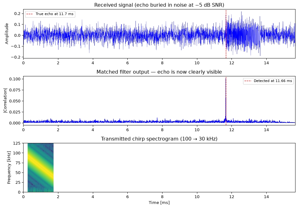
import numpy as npimport matplotlib.pyplot as pltimport syssys.path.insert(0, '.')from matched import simulate_bat_echo, detect_echo, make_chirpfrom scipy import signal as sig# Simulate a bat detecting a target at 2 metres, echo at -5 dB SNRfs =250000t, tx, rx, true_delay = simulate_bat_echo( fs=fs, target_distance=2.0, snr_db=-5.0, rng=np.random.default_rng(42))# Matched filter detectionn_chirp =int(0.002* fs)template = tx[:n_chirp]est_delay, mf_output = detect_echo(template, rx, fs)fig, axes = plt.subplots(3, 1, figsize=(10, 7))# Received signalaxes[0].plot(t *1000, rx, 'b-', linewidth=0.3)axes[0].axvline(true_delay *1000, color='red', linestyle='--', linewidth=1, label=f'True echo at {true_delay*1000:.1f} ms')axes[0].set_ylabel('Amplitude')axes[0].set_title('Received signal (echo buried in noise at −5 dB SNR)')axes[0].legend(fontsize=8)# Matched filter outputt_mf = np.arange(len(mf_output)) / fsaxes[1].plot(t_mf *1000, np.abs(mf_output), 'b-', linewidth=0.5)axes[1].axvline(est_delay *1000, color='red', linestyle='--', linewidth=1, label=f'Detected at {est_delay*1000:.2f} ms')axes[1].set_ylabel('|Correlation|')axes[1].set_title('Matched filter output — echo is now clearly visible')axes[1].legend(fontsize=8)# Spectrogram of transmitted chirpt_chirp, chirp = make_chirp(100000, 30000, 0.002, fs)f_spec, t_spec, Sxx = sig.spectrogram(chirp, fs, nperseg=128, noverlap=120)axes[2].pcolormesh(t_spec *1000, f_spec /1000, 10* np.log10(Sxx +1e-20), shading='gouraud', cmap='viridis')axes[2].set_ylabel('Frequency [kHz]')axes[2].set_xlabel('Time [ms]')axes[2].set_title('Transmitted chirp spectrogram (100 → 30 kHz)')for ax in axes: ax.set_xlim(0, t[-1] *1000)fig.tight_layout()plt.show()
Figure 1: Bat echolocation simulation. Top: the received signal looks like pure noise. Middle: the matched filter output shows a clear peak at the echo delay. Bottom: spectrogram of the transmitted chirp.
The key result: the received signal looks like pure noise (top panel), but the matched filter output (middle panel) shows a sharp, unambiguous peak at the correct delay. This is the power of pulse compression: the chirp’s energy is concentrated into a single correlation peak.
Range resolution
The range resolution of the matched filter is determined by the chirp bandwidth, not its duration:
\[\Delta d = \frac{c}{2B}\]
For a bat chirp spanning \(B = 70\) kHz: \(\Delta d = 343 / (2 \times 70{,}000) \approx 2.5\) mm. This is why bats can distinguish individual insects.
Application: LIGO gravitational wave detection
LIGO uses matched filtering on a grand scale. The detector measures strain (fractional length change) in two 4 km laser interferometer arms. A passing gravitational wave causes differential stretching. The signal amplitude is \(\sim 10^{-21}\), far below the noise floor.
The detection pipeline:
Generate a template bank: ~250,000 waveforms from general relativity, parameterised by component masses and spins
Matched-filter the data against every template
The template with the highest SNR peak is the best candidate
Require coincident detection at both LIGO sites (Hanford and Livingston)
The first detection (GW150914) had a matched filter SNR of ~24, clearly above the detection threshold of ~8. The template that matched corresponded to two black holes of ~36 and ~29 solar masses merging 1.3 billion light-years away.
This application highlights two challenges at scale:
Computational cost: correlating against 250,000 templates in real time requires GPU clusters and FFT-based matched filtering
Colored noise: LIGO noise is far from white (dominated by seismic noise below 10 Hz, thermal noise around 100 Hz, shot noise above 1 kHz). The optimal filter in colored noise is the prewhitened matched filter: whiten the data first, then correlate. This connects to the noise whitening topic.
Matched filter in colored noise
The derivation above assumes white noise. When the noise has a known power spectral density \(S_v(f)\), the optimal filter becomes:
\[H_\text{opt}(f) = \frac{S^*(f)}{S_v(f)}\]
This is equivalent to:
Prewhiten both the received signal and the template by filtering with \(1/\sqrt{S_v(f)}\)
Apply the standard matched filter to the whitened signals
Frequencies where the noise is low contribute more to detection: the filter automatically emphasises the “cleanest” parts of the spectrum.
Comparison with energy detection
An alternative to matched filtering is energy detection: simply measure the total energy in a time window and compare to a threshold. This requires no knowledge of the signal shape.
Property
Matched filter
Energy detector
Requires known template
Yes
No
Optimal for known signals
Yes (maximises SNR)
No
Works for unknown signals
No
Yes
Computational cost
\(O(N \log N)\) with FFT
\(O(N)\)
Sensitivity
High
Low
When the signal shape is known, matched filtering always wins. When it is unknown, energy detection or more general approaches (spectrograms, wavelets) are needed.
Template mismatch. Real-world signals never exactly match the template (Doppler shift in radar, dispersion in underwater acoustics, waveform uncertainty in LIGO). Mismatch degrades the output SNR. How much mismatch can be tolerated before the matched filter loses its advantage over simpler detectors?
Multiple targets. When multiple echoes overlap, matched filter sidelobes from one target can mask weaker targets. Window functions (Hamming, Chebyshev) on the chirp reduce sidelobes but broaden the main peak, the classic resolution-sidelobe trade-off.
Adaptive matched filtering. When the noise statistics are unknown or non-stationary, combining matched filtering with adaptive noise estimation is an active research area. This connects to adaptive filtering.
References
Source Code
---title: "Matched Filtering"subtitle: "Detecting known signals in noise: from bat echolocation to gravitational waves"---In 2015, the LIGO observatory detected a gravitational wave from two colliding black holes 1.3 billion light-years away. The signal was so faint that it was buried far below the noise floor. How did they find it? They correlated the measured data against a bank of 250,000 template waveforms, one for each possible combination of black hole masses and spins. The template that produced the largest correlation peak was the detection. This technique is called **matched filtering**, and it is provably optimal: no other linear filter can achieve a higher output signal-to-noise ratio.The same principle explains how bats navigate in complete darkness. A bat emits a frequency-modulated chirp and listens for echoes. Its auditory system performs something functionally equivalent to matched filtering (correlating the returning sound with the expected chirp shape) to achieve the extraordinary range resolution needed to catch insects mid-flight.Radar, sonar, GPS, wireless communications, and medical ultrasound all use the same idea. The matched filter is one of the most widely deployed algorithms in signal processing.::: {.callout-note title="Prerequisites"}This topic assumes familiarity with [convolution](../../basics/02-discrete-time.qmd#convolution), the [frequency domain](../../basics/05-frequency-domain.qmd), and [SNR](../../basics/03-noise-snr.qmd).:::---## The setupYou know the shape of the signal you are looking for (the **template**), but not *when* it arrives or *whether* it is present. The received signal is:$$r[n] = \alpha \cdot s[n - n_0] + v[n]$$where $s[n]$ is the known template, $\alpha$ is an unknown amplitude, $n_0$ is the unknown arrival time, and $v[n]$ is additive noise. The goal is to find $n_0$ (and decide whether the signal is present at all).---## Derivation: maximising output SNRWe want a filter $h[n]$ of length $N$ that maximises the **peak output SNR**, the ratio of the peak signal power at the output to the average noise power at the output.The filter output is:$$y[n] = \sum_{k=0}^{N-1} h[k] \, r[n-k]$$At the moment the template is aligned ($n = n_0 + N - 1$), the signal component of the output is:$$y_s = \alpha \sum_{k=0}^{N-1} h[k] \, s[N-1-k] = \alpha \, \mathbf{h}^T \mathbf{s}_\text{rev}$$where $\mathbf{s}_\text{rev}$ is the time-reversed template. The noise output power is:$$P_\text{noise} = \sigma_v^2 \sum_{k=0}^{N-1} h[k]^2 = \sigma_v^2 \|\mathbf{h}\|^2$$The output SNR is:$$\text{SNR}_\text{out} = \frac{y_s^2}{P_\text{noise}} = \frac{\alpha^2 (\mathbf{h}^T \mathbf{s}_\text{rev})^2}{\sigma_v^2 \|\mathbf{h}\|^2}$$By the **Cauchy–Schwarz inequality**, $(\mathbf{h}^T \mathbf{s}_\text{rev})^2 \leq \|\mathbf{h}\|^2 \|\mathbf{s}_\text{rev}\|^2$, with equality when $\mathbf{h} = c \cdot \mathbf{s}_\text{rev}$ for any constant $c$. Therefore, the filter that maximises output SNR is:$$\boxed{h[n] = s[N-1-n]}$$The optimal filter is the **time-reversed template**. Filtering with $h[n]$ is equivalent to computing the cross-correlation of the received signal with the template.The maximum achievable output SNR is:$$\text{SNR}_\text{out,max} = \frac{\alpha^2}{\sigma_v^2} \sum_{k=0}^{N-1} s[k]^2 = \frac{\alpha^2 E_s}{\sigma_v^2}$$where $E_s$ is the template energy. The output SNR depends only on the total energy of the template, not on its shape: a longer or louder signal gives better detection regardless of waveform.---## Cross-correlation equivalenceThe matched filter output can be written as:$$y[n] = \sum_{k=0}^{N-1} s[k] \, r[n - (N-1) + k] = (r \star s)[n]$$This is the **cross-correlation** of $r$ with $s$. In many implementations, matched filtering is computed as correlation rather than convolution: the two are identical when the filter is the time-reversed template.In the frequency domain:$$Y(f) = S^*(f) \cdot R(f)$$where $S^*$ is the complex conjugate of the template's spectrum. This leads to efficient FFT-based implementations for long signals.---## Pulse compressionA remarkable consequence: you can transmit a long, low-power signal and achieve the same detection performance as a short, high-power pulse. The matched filter **compresses** the extended signal into a sharp peak at the output.The **compression ratio** is approximately equal to the **time-bandwidth product**:$$\text{CR} \approx B \cdot T$$where $B$ is the signal bandwidth and $T$ is its duration. A chirp sweeping 70 kHz in 2 ms has $\text{CR} \approx 140$: the matched filter output peak is 140 times narrower than the original signal.This is why bats use chirps rather than clicks: a chirp spreads the same energy over a longer time (keeping the instantaneous power within biological limits) while the auditory system's correlation processing recovers the range resolution of a much shorter pulse.### Processing gainPulse compression buys SNR, not just resolution. The derivation above gave the peak output SNR as $\alpha^2 E_s / \sigma_v^2$: every sample of the template adds coherently at the alignment instant while the noise adds incoherently, so a longer, wider chirp wins on both counts. Expressed as a gain of output SNR over input SNR, this **processing gain** is approximately the same time-bandwidth product:$$G \approx B \cdot T$$The [front-page bat figure](../../index.qmd) uses an FM chirp sweeping $B = 55$ kHz over $T = 4$ ms, so $B \cdot T = 220$, a predicted gain of $10 \log_{10}(220) \approx 23$ dB. This is real, not a plotting trick: a Monte-Carlo simulation of that exact chirp (echo amplitude 0.5 in unit-variance noise, 400 trials) measures a mean gain of **23.5 dB** when the input SNR is referenced to the signal band $B$, within rounding of the prediction. That is the whole story of the landing-page demo: an echo sitting near $-4$ dB in the raw trace becomes a peak roughly 20 dB above the noise floor.::: {.callout-warning title="What 'gain' means here"}The exact dB figure depends on how you define the *input* SNR. Referenced to the signal band $B$, the gain is $\approx B \cdot T$ (above). Referenced to a single sample, it is instead the number of samples in the pulse, $N = T f_s$ (here 1000, or 30 dB), minus a few dB for the Hanning taper's energy loss. Same physics, different denominator. Quote the bandwidth you are measuring in.:::---## Application: bat echolocationA bat hunting in the dark faces a classic detection problem:1. Emit a frequency-modulated (FM) chirp, typically sweeping from ~100 kHz down to ~30 kHz in 1–5 ms2. Listen for echoes from prey and obstacles3. Estimate the range from the echo delay: $d = c \cdot \tau / 2$, where $c \approx 343$ m/sThe echo is severely attenuated (sound intensity falls as $1/r^4$ for a reflected signal) and mixed with noise from wind, other bats, and environmental sounds. The bat needs to detect echoes at SNRs well below 0 dB.The simulation below models this scenario using the matched filter implementation in [`matched.py`](matched.py):```{python}#| label: fig-bat-echo#| fig-cap: "Bat echolocation simulation. Top: the received signal looks like pure noise. Middle: the matched filter output shows a clear peak at the echo delay. Bottom: spectrogram of the transmitted chirp."import numpy as npimport matplotlib.pyplot as pltimport syssys.path.insert(0, '.')from matched import simulate_bat_echo, detect_echo, make_chirpfrom scipy import signal as sig# Simulate a bat detecting a target at 2 metres, echo at -5 dB SNRfs =250000t, tx, rx, true_delay = simulate_bat_echo( fs=fs, target_distance=2.0, snr_db=-5.0, rng=np.random.default_rng(42))# Matched filter detectionn_chirp =int(0.002* fs)template = tx[:n_chirp]est_delay, mf_output = detect_echo(template, rx, fs)fig, axes = plt.subplots(3, 1, figsize=(10, 7))# Received signalaxes[0].plot(t *1000, rx, 'b-', linewidth=0.3)axes[0].axvline(true_delay *1000, color='red', linestyle='--', linewidth=1, label=f'True echo at {true_delay*1000:.1f} ms')axes[0].set_ylabel('Amplitude')axes[0].set_title('Received signal (echo buried in noise at −5 dB SNR)')axes[0].legend(fontsize=8)# Matched filter outputt_mf = np.arange(len(mf_output)) / fsaxes[1].plot(t_mf *1000, np.abs(mf_output), 'b-', linewidth=0.5)axes[1].axvline(est_delay *1000, color='red', linestyle='--', linewidth=1, label=f'Detected at {est_delay*1000:.2f} ms')axes[1].set_ylabel('|Correlation|')axes[1].set_title('Matched filter output — echo is now clearly visible')axes[1].legend(fontsize=8)# Spectrogram of transmitted chirpt_chirp, chirp = make_chirp(100000, 30000, 0.002, fs)f_spec, t_spec, Sxx = sig.spectrogram(chirp, fs, nperseg=128, noverlap=120)axes[2].pcolormesh(t_spec *1000, f_spec /1000, 10* np.log10(Sxx +1e-20), shading='gouraud', cmap='viridis')axes[2].set_ylabel('Frequency [kHz]')axes[2].set_xlabel('Time [ms]')axes[2].set_title('Transmitted chirp spectrogram (100 → 30 kHz)')for ax in axes: ax.set_xlim(0, t[-1] *1000)fig.tight_layout()plt.show()```The key result: the received signal looks like pure noise (top panel), but the matched filter output (middle panel) shows a sharp, unambiguous peak at the correct delay. This is the power of pulse compression: the chirp's energy is concentrated into a single correlation peak.::: {.callout-note}## Range resolutionThe range resolution of the matched filter is determined by the chirp bandwidth, not its duration:$$\Delta d = \frac{c}{2B}$$For a bat chirp spanning $B = 70$ kHz: $\Delta d = 343 / (2 \times 70{,}000) \approx 2.5$ mm. This is why bats can distinguish individual insects.:::---## Application: LIGO gravitational wave detectionLIGO uses matched filtering on a grand scale. The detector measures strain (fractional length change) in two 4 km laser interferometer arms. A passing gravitational wave causes differential stretching. The signal amplitude is $\sim 10^{-21}$, far below the noise floor.The detection pipeline:1. Generate a template bank: ~250,000 waveforms from general relativity, parameterised by component masses and spins2. Matched-filter the data against every template3. The template with the highest SNR peak is the best candidate4. Require coincident detection at both LIGO sites (Hanford and Livingston)The first detection (GW150914) had a matched filter SNR of ~24, clearly above the detection threshold of ~8. The template that matched corresponded to two black holes of ~36 and ~29 solar masses merging 1.3 billion light-years away.This application highlights two challenges at scale:- **Computational cost**: correlating against 250,000 templates in real time requires GPU clusters and FFT-based matched filtering- **Colored noise**: LIGO noise is far from white (dominated by seismic noise below 10 Hz, thermal noise around 100 Hz, shot noise above 1 kHz). The optimal filter in colored noise is the *prewhitened* matched filter: whiten the data first, then correlate. This connects to the [noise whitening topic](../noise-whitening/index.qmd).---## Matched filter in colored noiseThe derivation above assumes white noise. When the noise has a known power spectral density $S_v(f)$, the optimal filter becomes:$$H_\text{opt}(f) = \frac{S^*(f)}{S_v(f)}$$This is equivalent to:1. **Prewhiten** both the received signal and the template by filtering with $1/\sqrt{S_v(f)}$2. Apply the standard matched filter to the whitened signalsThe output SNR in colored noise is:$$\text{SNR}_\text{out} = \alpha^2 \int \frac{|S(f)|^2}{S_v(f)} df$$Frequencies where the noise is low contribute more to detection: the filter automatically emphasises the "cleanest" parts of the spectrum.---## Comparison with energy detectionAn alternative to matched filtering is **energy detection**: simply measure the total energy in a time window and compare to a threshold. This requires no knowledge of the signal shape.| Property | Matched filter | Energy detector ||---|---|---|| Requires known template | Yes | No || Optimal for known signals | Yes (maximises SNR) | No || Works for unknown signals | No | Yes || Computational cost | $O(N \log N)$ with FFT | $O(N)$ || Sensitivity | High | Low |When the signal shape is known, matched filtering always wins. When it is unknown, energy detection or more general approaches (spectrograms, wavelets) are needed.---## ImplementationSee [`matched.py`](matched.py) for implementations:- `matched_filter()`: direct cross-correlation- `matched_filter_fft()`: FFT-based (efficient for long signals)- `make_chirp()`: generate FM chirp signals- `simulate_bat_echo()`: full bat echolocation simulation- `detect_echo()`: estimate echo delay from matched filter peakFor hardware implementations of chirp generation and matched filtering, see [Matched Filtering on Hardware](embedded.qmd).---## Open questions- **Template mismatch.** Real-world signals never exactly match the template (Doppler shift in radar, dispersion in underwater acoustics, waveform uncertainty in LIGO). Mismatch degrades the output SNR. How much mismatch can be tolerated before the matched filter loses its advantage over simpler detectors?- **Multiple targets.** When multiple echoes overlap, matched filter sidelobes from one target can mask weaker targets. Window functions (Hamming, Chebyshev) on the chirp reduce sidelobes but broaden the main peak, the classic resolution-sidelobe trade-off.- **Adaptive matched filtering.** When the noise statistics are unknown or non-stationary, combining matched filtering with adaptive noise estimation is an active research area. This connects to [adaptive filtering](../adaptive-filtering/index.qmd).## References::: {#refs}:::